CT Protocol Optimization over the TOPICS: Range of …amos3.aapm.org/abstracts/pdf/68-19861-237357-85774.pdfCT Protocol Optimization over the ... Computed Tomography Quick Overview

University of Wisconsin CT Talk 9/26/11

1

9/26/11 1© 2012, Frank Ranallo

CT Protocol Optimization over the

Range of CT Scanner Types: Recommendations & Misconceptions

Frank N. Ranallo, Ph.D.

Associate Professor of Medical Physics & Radiology

University of Wisconsin – School of Medicine & Public Health

TOPICS: Computed Tomography Quick Overview

CT Dosimetry

CT Image Quality

Optimization of CT Scan Techniques for Dose & Image Quality


Evolution to Helical/ Spiral CT Scanners

Single Slice Helical/ Spiral CT


Evolution to Multislice Scanners

2, 4, 8, 16, 64, … ?

Data Acquisition


2



2, 4, 8, 16, 64, … ?



2, 4, 8, 16, 64, … ?

Pitch =Table travel per 360° tube rotation__________________________________

Nominal Slice Thickness

Definition of Pitch for Single-slice Helical / Spiral Scanning

______________________________Pitch =

Total collimation width of all

simultaneously collected slices

Table travel per 360° tube rotation

Definition of Pitch for Multi-slice Helical / Spiral Scanning

9/26/11

CT Protocols

7© 2012, Frank Ranallo

Series 3 - Abdomen/ Pelvis

--Medium Adult--From Recon 1: Sa & Co Reformat:

Ave., 5.0 mm thick & 2.5 mm interval

CT 1 CT 2 CT 3 CT 4 & East & RP CT

Scanner GE LS Xtra GE LS 16 GE LS 16 Pro GE LS VCT 64 GE LS 8

Scan Type Helical Helical Helical Helical Helical

Rotation Time (sec) 0.5 0.5 0.5 0.5 0.5

Detector Coverage (mm)

Beam Collimation (mm)20 20 20 40 10

Detector Rows 16 16 16 64 8

Pitch 0.938 0.938 0.938 0.516 1.35

Speed (mm/rot) 18.75 18.75 18.75 20.64 13.5

Detector Configuration 16 x 1.25 16 x 1.25 16 x 1.25 64 x 0.625 8 x 1.25

Slice Thickness (mm) 1.25 1.25 1.25 1.25 1.25

Interval (mm) 0.625 0.625 0.625 0.625 0.625

Scan FOV Large Large Large Large Body Large

kV 120 120 120 120 120

Smart mA/ Auto mA Range 150-660 120-440 120-660 60-660 180-440

Noise Index 24 24 24 24 24

(Manual mA) 570 440 460 240 440

Recon 1:

DFOV 36 36 36 36 36

Recon Type Standard Standard Standard Standard Standard

WW/ WL 325/15 325/15 325/15 325/15 325/15

Recon Option Plus Plus Plus Plus Plus

Recon Option IQ Enhance

Recon 2:

DFOV 36 36 36 36 36


WW/ WL 325/15 325/15 325/15 325/15 325/15



Interval (mm) 3.0 3.0 3.0 3.0 3.0

9/26/11

CT Protocols


Series 3 - Abdomen/ Pelvis

--Medium Adult--From Recon 1: Sa & Co Reformat:

Ave., 5.0 mm thick & 2.5 mm interval


Scanner GE LS Xtra GE LS 16 GE LS 16 Pro GE LS VCT 64 GE LS 8

Scan Type Helical Helical Helical Helical Helical

Rotation Time (sec) 0.5 0.5 0.5 0.5 0.5

Detector Coverage (mm)

Beam Collimation (mm)20 20 20 40 10

Detector Rows 16 16 16 64 8

Pitch 0.938 0.938 0.938 0.516 1.35

Speed (mm/rot) 18.75 18.75 18.75 20.64 13.5

Detector Configuration 16 x 1.25 16 x 1.25 16 x 1.25 64 x 0.625 8 x 1.25


Interval (mm) 0.625 0.625 0.625 0.625 0.625

Scan FOV Large Large Large Large Body Large

kV 120 120 120 120 120

Smart mA/ Auto mA

Range150-660 120-440 120-660 60-660 180-440

Noise Index 24 24 24 24 24

(Manual mA) 570 440 460 240 440


3

9/26/11

CT Protocols



Recon 1:

DFOV 36 36 36 36 36


WW/ WL 325/15 325/15 325/15 325/15 325/15


Recon Option IQ Enhance

Recon 2:

DFOV 36 36 36 36 36


WW/ WL 325/15 325/15 325/15 325/15 325/15



Interval (mm) 3.0 3.0 3.0 3.0 3.0

Dose in

Computed

Tomography

RADIATION UNITS

New Old SI Units Conventional

Units

Absorbed Dose Units: gray (Gy) or rad (r)

Equivalent Dose Units: sievert (Sv) or rem

Effective Dose Units: sievert (Sv) or rem

RADIATION UNITS

Effective Dose

The concept of effective dose takes into account

the risk to the person exposed to radiation that

is not uniform over the entire body.

Different organs have different

sensitivities to radiation

This is expressed by the tissue

weighting factor: wT


4

CT Dose

CTDI

CTDI100 measured at the center of the

phantom is called CTDI100 (center)

CTDI100 measured near the surface of

the phantom is called CTDI100

(surface) or CTDI100 (peripheral)

CT Dose

CTDI

CTDIw is a weighted value of CTDI100

that attempts to give the average

dose throughout the volume of the

phantom (again, for contiguous axial

slices or for helical scanning at a

pitch of 1). It is defined as:

CTDIw = 1/3 CTDI100 (center) +

2/3 CTDI100 (surface)

CT Dose

CTDI

If you then take into account the

effect of pitch on dose for a helical/

spiral scan then you have another

version of CTDI:

This is an approximation of the dose

averaged over the volume of the phantom.

CTDIvol = CTDIw / Pitch

CT Dose

DLP

A final dosimetry measure is the

Dose Length Product (DLP) which is

defined as:

CTDIvol and DLP are the radiation

units provided by the CT Scanner.

DLP = CTDIvol Scan Length

and has units of mGy • cm


5

CT Dose

DLP

Estimates of a patient’s effective

dose (E) can be derived from the

values of DLP for an examination.

Use the following equation

containing a coefficient EDLP

appropriate to the examination:

E = EDLP × DLP

CT Dose DLP

Values of EDLP for Adult scans:

Region of Body EDLP (mSv / mGy•cm) Phantom

Head 0.0023 0.0021 16 cm

Head & Neck 0.0031 16 cm

Neck 0.0054 0.0059 32 cm

Chest 0.017 0.014 32 cm

Abdomen 0.015 0.015 32 cm

Pelvis 0.019 0.015 32 cm

Two different sources

CT Dose

Converting DLP to Effective Dose

for Adults

Quick method of getting the effective

dose in mSv from the DLP in mGy•cm:

Take the DLP and divide it by 100

For the Body, then multiply by 1.5

For the Head, then divide by 4


6

Image Quality in

Computed

Tomography

Image Quality and Dose:

Dose

Image

Sharpness

Image

Noise

Low Contrast

DetectabilityArtifacts

9/26/11 23

Image Reconstruction Filters, Algorithms,

or KernelsBelow are the measured MTF functions for the reconstruction algorithms available on a

GE scanner. The algorithms that do not have a "hump" in the MTF are: soft, standard,

detail, bone, and edge in order of increasing sharpness. A hump in the MTF indicates a

form of edge enhancement of the image; these are evident in the lung reconstruction

and the bone plus reconstruction.

0.0

0.2

0.4

0.6

0.8

1.0

1.2

1.4

1.6

1.8

0.0 2.0 4.0 6.0 8.0 10.0 12.0 14.0 16.0

v (cycles/cm)

MT

F (

v)

Soft

Standard

Detail

Bone

Bone Plus

Edge

Lung

© 2012, Frank Ranallo 9/26/11 24

Image Reconstruction Filters, Algorithms,

or Kernels (Siemens)•Kernel names have 4 positions. Example: B31s.

•Pos.1: kernel type (B=body, C=child head, H=head, U=ultra high resolution, S=special kernel, T=topo.)

Pos. 2: resolution (1,...,9. Higher number -> higher resolution)

•Pos. 3: version (0,...,9)

•Pos. 4: scan mode (f=fast (no j-FFS , no UHR comb), s=standard (with j-FFS , no UHR comb), h=highres (with j-FFS, no UHR comb),

u=ultrahighres (with j-FFS, with UHR comb))

•The use of z-FFS is not coded to the kernel name.

B10f, B18f, B19f, B20f, B25f, B29f, B30f, B31f, B35f, B36f, B39f, B40f,

B41f, B45f, B46f, B47f, B50f, B60f, B65f, B70f, B75f, B80f,

B08s, B10s, B18s, B19s, B20s, B25s, B29s, B30s, B31s, B35s, B39s,

B40s, B41s, B45s, B46s, B47s, B50s, B60s, B65s, B70s, B75h, B80s.

B30m/B40m (m=f,s) are standard kernels,

B20m/B10m are more smooth.

Br1m (r=3,4) have about the same visual sharpness as Br0m, but a

finer noise structure (better image impression, improved LC).

B25m correspond to kernels B30m with ASA.

B35m is designed for Ca-scoring and quantitative analysis,

B36f is a sharper version of B35f,

B45m has intermediate resolution.

B46m is for investigations of patency of stents and for quantitative

investigations.

B47m have resolution between B46m and B50m.

B50m, B60m, B70m are sharper kernels (for cervical spine, shoulder,

extremities, thorax).

B65m is a special lungHR-kernel for quantitative evaluations.

B80m is a special lungHR-kernel (corresponding to HCE with B40m);

not as sharp as B70m.

B18m are the kernels B10m with stronger de-ringing.

Br9m (r=1,2,3) are the PET/SPECT versions of Br0m.

B75m (m=f,h) are lungHR kernels with less overshooting at edges.

H10f, H19f, H20f, H21f, H22f, H23f, H29f, H30f, H31f,

H32f, H37f, H39f, H40f, H41f, H42f, H45f, H47f, H48f,

H50f, H60f,

H10s, H19s, H20s, H21s, H22s, H23s, H29s, H30s,

H31s, H32s, H37s, H39s, H40s, H41s, H42s, H45s,

H47s, H48s, H50s, H60s,

H70h, H80h (Open only).

H40m (m=f, s) is the standard kernel,

H30m, H20m or H10m lead to softer images.

Hr1m (r=2,3,4) yield the same visual sharpness as

Hr0m, but have a finer noise structure (better image

impression, improved LC). Therefore Hr1m are used

in standard protocols.

Hr2m are the kernels Hr0m without PFO.

H23m serves for Neuro PBV.

H37m, H47m, H48m are alternative kernels with

different noise impression.

H45m serve for intermediate resolution,

H50m, H60m are sharper kernels.

Hr9m (r=1,2,3) are the PET/SPECT versions of Hr0m.

H70h gives highest resolution without comb.

H80h gives the hires specification for Sensation

Open.

© 2012, Frank Ranallo


7

Image Sharpness:

Images of a

resolution

pattern made

with different

Image

Reconstruction

Algorithms

Image Noise:

Images of a

uniform

water pattern

imaged using

mAs values

incrementing

by a factor

of 2, from

50 mAs to

1600 mAs.

Low Contrast Detectability:

Images of a

low contrast

detectability

pattern

imaged using

mAs values

incrementing

by a factor

of 2, from

50 mAs to

1600 mAs.

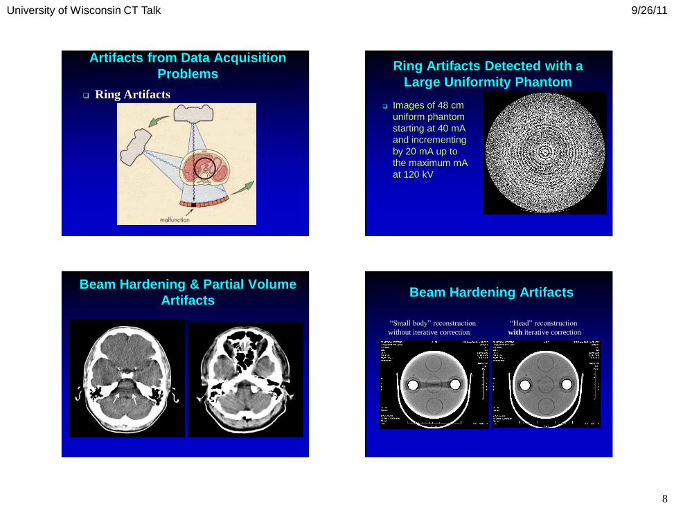
Artifacts from Data Acquisition

Problems

Ring Artifacts


8

Artifacts from Data Acquisition

Problems

Ring Artifacts

Ring Artifacts Detected with a

Large Uniformity Phantom

Images of 48 cm

uniform phantom

starting at 40 mA

and incrementing

by 20 mA up to

the maximum mA

at 120 kV

Beam Hardening & Partial Volume

ArtifactsBeam Hardening Artifacts

“Small body” reconstruction

without iterative correction

“Head” reconstruction

with iterative correction


9

Motion Artifacts

No Motion With Motion

Artifact due to the patient extending

outside the Scan Field of View;

ALSO “Stringy” noise artifact

9/26/11 35© 2012, Frank Ranallo

Effect of CT

Protocols on

Image Quality and

Dose


10

Axial Scan Techniques

Affecting Image Quality & Dose

kV

mAs – mA & scan time

Slice thickness

Helical Scan Techniques


kV

mAs – mA & scan time

Slice thickness

Pitch



Definition of Pitch for

Multislice Helical / Spiral Scanning:

______________________________Pitchcoll =

Total collimation width of all

simultaneously collected slices

Table travel per 360° tube rotation



Some scanners when using helical or spiral CT

use the concept of “effective mAs”

Effective mAs = mAs / pitch

To make things even more confusing, some

scanners (Philips) call the effective mAs in

helical scanning simply the “mAs”


11

Manual vs. Automatic Exposure

They did not contain any type of “phototimer” or

automatic exposure control (AEC) to assure a

proper patient dose.

Therefore, manual technique charts were needed

for different patient sizes.

Usually this was not done so that techniques more

suited for larger patients were used on all patients

resulting in unneeded radiation exposure.

One big defect of CT Scanners before 2001

9/26/11 42

Automatic Exposure Control in CT Scanners

Most modern CT scanners have some type of

automatic exposure control (AEC) that changes

the mA during the scan.

There are two basic types of AEC that can be

used separately or together:

The scanner varies the mA at different axial

positions of the patient.

The scanner varies the mA as the tube

rotates around the patient.

It is usually optimal to use both types together

if the scanner allows it.


9/26/11 43



The scanner varies the mA

at different axial positions

of the patient.

The scanner varies the mA

at different axial positions

of the patient and also

varies the mA as the tube

rotates around the patient.

9/26/11 44


Caution: The methods used by different

manufacturers to perform AEC in CT are

very different and may achieve very

different clinical results.



12

9/26/11 45


Some scanners (GE, Toshiba) try to keep the

image noise constant as patient size increases:

the automatic exposure control is adjusted by

selecting the amount of noise that you wish

in the image. This is done by selecting a

“Noise Index” or “SD” (standard deviation).

Typical values of Noise Index are 2.5 to 3.5 for

a standard adult head scan and 12 to 20 for

the body.

The scanner attempts to keep the image noise

constant by adjusting the mA within set limits.

© 2012, Frank Ranallo 9/26/11 46



GE:With GE scanners you

must select whether

you will be using

manual techniques

“Manual mA” or AEC

techniques “Auto mA”.

One uses an actual mA

setting, the other uses

a Noise Index setting.

Having one set

correctly in a protocol

does nothing to insure

the other is properly

set.

9/26/11 47


Other scanners (Siemens, Philips) allow you to

select the “mAs” or the “Effective mAs” that you

would use for an average size patient. For

Siemens scanners this selection is called the

“Quality reference mAs”.

Then the scanner automatically increases or

decreases the effective mAs for larger or smaller

patients. This is done by varying the mA.

Effective mAs = (mA x rotation time) / pitch

© 2012, Frank Ranallo 9/26/11 48



Siemens:With Siemens

scanners you select

the “eff. mAs” whether

you will be using

manual techniques

OR AEC techniques.

In manual mode this is

the actual eff. mAs

used and in AEC mode

it is the eff. mAs that

you would desire for

an “average” size

patient. There is not

the use of 2 different

parameters for manual

& AEC mode.


13

9/26/11 49


Scanners that try to keep the image noise

constant have the problem that they can quickly

reach the maximum mA “ceiling” before getting

to very large patients

Scanners that use a reference mAs setting will

generally allow the mA to increase only modestly

with increased patient size, allowing the image

noise to increase substantially for large patients

What is needed is a new hybrid approach.

© 2012, Frank Ranallo 9/26/11 50


A Siemens Problem:

After performing the topo scan, Siemens scanners warn

you if the available effective mAs is lower than the

effective mAs requested by the automatic exposure

control system, which will result in unacceptable image

quality.

However the scanner does not let you increase the kV

from 120 to 140 which could solve the problem!

This means a “work-around” is required: temporarily

reduce the Quality Ref mAs to a very low value. You can

then raise the kV to 140. Then increase the Quality Ref

mAs to at least ½ of its original value, if possible.


9/26/11 51


A GE (and Toshiba) Problem:

Since the GE scanner requires two separate parameters

for determining the mA in manual and AEC mode, one

must understand the application and use of the “Noise

Index” parameter when using AEC.

When switching from manual to AEC mode or from AEC

to manual mode one must be sure that the exposure

parameter of “manual mA” or “Noise Index” is properly

adjusted. When one of these modes is the

manufacturer’s “default” mode one cannot assume that

correct settings will result when switching modes.



Increasing the kV will have different

effects when using manual exposure

mode and different types of automatic

exposure modes.


14


In a manual mode increasing the kV will always

increase the patient dose, if all other scan

parameters are kept constant

With GE and Toshiba scanners, increasing the

kV in AEC mode will decrease the patient dose,

if all other scan parameters are kept constant

With Siemens and Philips scanners, increasing

the kV in AEC mode will increase the patient

dose, if all other scan parameters are kept

constant9/26/11 54© 2012, Frank Ranallo

Optimizing

CT Protocols:

Misconceptions

and

Recommendations

for

Scan and Imaging Parameters

kV

Misconceptions:

Scanning at 140 kV will reduce patient

dose for any type of CT scan: head, body,

adult or pediatric.

For head scans, 140 kV should be used

through the posterior fossa region to

reduce image artifacts from bone.


15

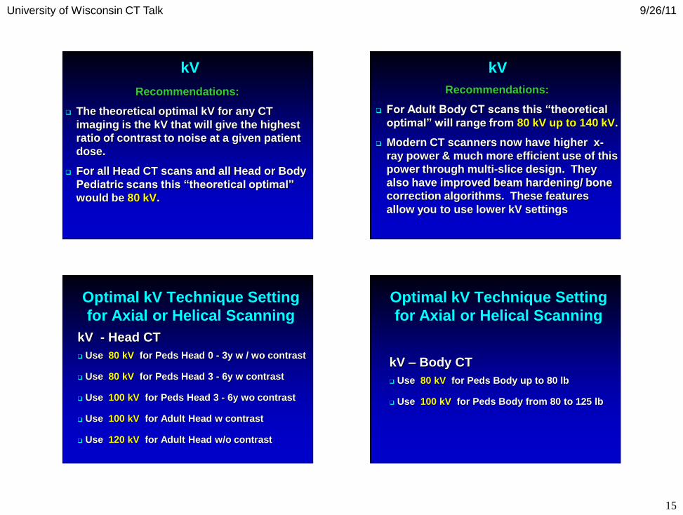
kV

Recommendations:

The theoretical optimal kV for any CT

imaging is the kV that will give the highest

ratio of contrast to noise at a given patient

dose.

For all Head CT scans and all Head or Body

Pediatric scans this “theoretical optimal”

would be 80 kV.

kV

Recommendations:

For Adult Body CT scans this “theoretical

optimal” will range from 80 kV up to 140 kV.

Modern CT scanners now have higher x-

ray power & much more efficient use of this

power through multi-slice design. They

also have improved beam hardening/ bone

correction algorithms. These features

allow you to use lower kV settings

Optimal kV Technique Setting

for Axial or Helical Scanning

kV - Head CT

Use 80 kV for Peds Head 0 - 3y w / wo contrast

Use 80 kV for Peds Head 3 - 6y w contrast

Use 100 kV for Peds Head 3 - 6y wo contrast

Use 100 kV for Adult Head w contrast

Use 120 kV for Adult Head w/o contrast

Optimal kV Technique Setting


kV – Body CT

Use 80 kV for Peds Body up to 80 lb

Use 100 kV for Peds Body from 80 to 125 lb


16

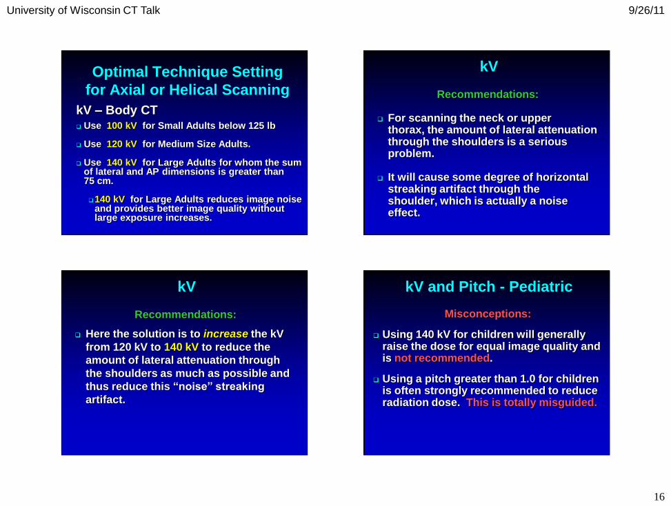
Optimal Technique Setting


kV – Body CT Use 100 kV for Small Adults below 125 lb

Use 120 kV for Medium Size Adults.

Use 140 kV for Large Adults for whom the sum of lateral and AP dimensions is greater than 75 cm.

140 kV for Large Adults reduces image noise and provides better image quality without large exposure increases.

kV

Recommendations:

For scanning the neck or upper thorax, the amount of lateral attenuation through the shoulders is a serious problem.

It will cause some degree of horizontal streaking artifact through the shoulder, which is actually a noise effect.

kV

Recommendations:

Here the solution is to increase the kV

from 120 kV to 140 kV to reduce the

amount of lateral attenuation through

the shoulders as much as possible and

thus reduce this “noise” streaking

artifact.

kV and Pitch - Pediatric

Misconceptions:

Using 140 kV for children will generally raise the dose for equal image quality and is not recommended.

Using a pitch greater than 1.0 for children is often strongly recommended to reduce radiation dose. This is totally misguided.


17

Pitch

Misconceptions

Scanning at higher pitch should be used

as a strategy to reduce patient dose and

is the best way to reduce scan time and

motion artifact and blur.

WRONG!!!

Pitch

Misconceptions:

A pitch of less than one over-irradiates

the patient due to scanning overlap.

Thus one should avoid using a pitch less

than one, particularly in pediatric scans.

WRONG!!!

Pitch

Recommendations:

Changing the pitch from 1.0 to 0.5

increases the patient dose by a factor of

2 but also decreases image noise.

The effects on dose and noise are the

same as increasing the mA or the

rotation time by a factor of 2, but with

the added advantage of decreasing

helical artifacts.

Pitch

Recommendations:

The effect of increased dose at lower

pitch is easily countered by reducing

the rotation time or mA in manual mode.

There is NO increase in dose when

decreasing pitch in AEC mode since the

AEC mode in all scanners will keep the

dose constant.


18

Pitch

Recommendations:

Lowering the pitch and decreasing the

exposure time by the same factor will

keep the patient dose and exam time

constant, but provide better image

quality – you get something for nothing!

Pitch

Recommendations:

Example:

Change a 1.0 sec rotation time

and a pitch of 1.1 to

a 0.5 sec rotation time

and a pitch of 0.55

Pitch

Recommendations:

For head scanning ALWAYS use a pitch

of less than 1.0 to minimize helical

artifact.

Best results are usually with a pitch just

above 0.5: 1 .

Pitch

Recommendations:

For body scanning use a pitch of less than

1.0 whenever possible to minimize helical

artifact and allow more radiation for the

adequate imaging of larger patients.

When decreasing pitch in body scans, you

need to be aware of breath hold limitations

and contrast considerations .


19

Pitch

Recommendations:

Many people believe that increasing

pitch is a proper dose reduction

strategy – It is NOT!

PitchRecommendations:

Instead of increasing pitch, the proper dose

reduction strategy is:

1. Reduce the rotation time (will reduce dose in

manual mode and is the first step in AEC mode).

2. Reduce the effective mAs (in manual or AEC

mode), reduce the mA (in manual mode, or

increase the noise index (in AEC mode).

3. Only then increase pitch if required to reduce

total exam time.

9/26/11 75© 2012, Frank Ranallo

Axial vs. Helical Scanning

Misconceptions:

Heads should always be scanned using

the axial rather than the helical mode or

you will get a lower quality image.


20

Axial vs. Helical ScanningRecommendations:

Helical scanning will almost always allow

an exam with equal or better image quality

than an axial scan if you have a CT scanner

with 16 or more slices and select proper

scan techniques.

Axial scanning is still useful if required for

positioning of the patient to avoid artifacts,

since tilting the gantry is not allowed with

helical scanning.


and slice reconstruction interval

Recommendations:

Advantages of Helical scanning:

Shorter total scan time with less chance

for patient motion during the scan.

The ability to reconstruct slices at

intervals less than the slice thickness.

VERY IMPORTANT!

Recommendations:

With axial scanning, the slice

reconstruction incrementation is

normally equal to the slice thickness.



Recommendations:

With helical scanning, the slice recon-

struction incrementation can be set at any

value. The best z-resolution is obtained by

reconstructing at intervals ½ of the actual

slice thickness – this particularly helps with

multiplanar reformatting.

This is a significant advantage of helical

scanning that is often not utilized.




21

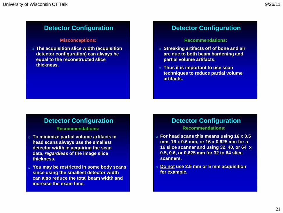
Detector Configuration

Misconceptions:

The acquisition slice width (acquisition

detector configuration) can always be

equal to the reconstructed slice

thickness.

Detector Configuration

Recommendations:

Streaking artifacts off of bone and air

are due to both beam hardening and

partial volume artifacts.

Thus it is important to use scan

techniques to reduce partial volume

artifacts.

Detector ConfigurationRecommendations:

To minimize partial volume artifacts in

head scans always use the smallest

detector width in acquiring the scan

data, regardless of the image slice

thickness.

You may be restricted in some body scans

since using the smallest detector width

can also reduce the total beam width and

increase the exam time.


For head scans this means using 16 x 0.5

mm, 16 x 0.6 mm, or 16 x 0.625 mm for a

16 slice scanner and using 32, 40, or 64 x

0.5, 0.6, or 0.625 mm for 32 to 64 slice

scanners.

Do not use 2.5 mm or 5 mm acquisition

for example.


22


With a GE 16 slice scanner you can use a

16 x 0.625 acquisition for the best quality

in the head, but this only gives you a 10

mm beam width.

In the body you may need to go to a 16 x

1.25 acquisition which provides a 20 mm

beam width and allows you to scan at

twice the speed.


However the 16 slice GE scanner also

allows you to use it in an 8 slice mode:

8 x 1.25 mm or 8 x 2.5 mm - which

should NEVER BE USED.

Likewise the GE 8 slice scanner can

also be used in a 4 slice mode - which

again should NEVER BE USED.

9/26/11 87© 2012, Frank Ranallo 9/26/11 88© 2012, Frank Ranallo


23

With a manual technique of 120

kV, 600 mA, 0.5 sec, 0.75 pitch, what

is the effective mAs used in this scan

?

0%

0%

0%

0%

0%

10

1. 600 mAs

2. 300 mAs

3. 450 mAs

4. 400 mAs

5. 225 mAs

With a manual technique of 120 kV,

600 mA, 0.5 sec, 0.75 pitch, what is

the effective mAs used in this scan ?

0%

0%

0%

0%

0%

10

1. 600 mAs

2. 300 mAs

3. 450 mAs

4. 400 mAs

5. 225 mAs

Answer: 4. 400 mAs

Effective mAs = 600mA * 0.5s / 0.75 = 400

Ref: M Mahesh, MDCT Physics – The Basics (2009)

Which of the following changes in technique will

decrease the image noise by a factor of 2 ?

0%

0%

0%

0%

0%

10

1. Increase the slice thickness by a factor of 4


3. Decrease the slice thickness by a factor of 2

4. Decrease the mA by a factor of 2

5. Decrease the kV by 20 kV

Which of the following changes in technique will

decrease the image noise by a factor of 2 ?

0%

0%

0%

0%

0%

10



3. Decrease the slice thickness by a factor of 2

4. Decrease the mA by a factor of 2

5. Decrease the kV by 20 kV

Answer: 1. Increase the slice thickness by a factor of 4

Ref: M. McNitt-Gray, “AAPM/RSNA Physics Tutorial for Residents:

Topics in CT: Radiation Dose in CT,” RadioGraphics 2002; 22:1541–1553 .


24

For an AEC control that uses a quality reference

(or target) effective mAs (mAsQR), if you change

the kV from 120 to 80 and keep the mAsQR

constant, how will the dose change?

0%

0%

0%

0%

0%

10

1. Increase by about a factor of 1.5

2. Increase by about a factor of 3

3. Remain approximately the same

4. Decrease by about a factor of 1.5

5. Decrease by about a factor of 3

For an AEC control that uses a quality reference

(or target) effective mAs (mAsQR), if you change

the kV from 120 to 80 and keep the mAsQR


0%

0%

0%

0%

0%

10






Answer: 5. Decrease by about a factor of 3

Ref: Siemens Somatom Sensation Datasheet & Siemens

Somatom Sensation Application Guide

For an AEC control that uses a Noise Index (NI)

– or Standard Deviation (SD), if you change the

kV from 120 to 80 and keep the NI or SD


0%

0%

0%

0%

0%

10






For an AEC control that uses a Noise Index (NI)

– or Standard Deviation (SD), if you change the

kV from 120 to 80 and keep the NI or SD


0%

0%

0%

0%

0%

10






Answer: 2. Increase by about a factor of 3

Ref: H. Brisse, “Automated exposure control in multichannel CT with tube current

modulation to achieve a constant level of noise.” Med. Phys. 34 (7), July 2009.


25

Starting with a manual technique of 120 kV,

400 mA, 1.0 sec, 0.75 pitch, which is the best

way to reduce the dose by a factor of 2 ?

0%

0%

0%

0%

0%

10

1. 120 kV, 200 mA, 1.0 sec, 0.75 pitch

2. 120 kV, 400 mA, 1.0 sec, 1.5 pitch

3. 120 kV, 400 mA, 0.5 sec, 0.75 pitch

4. 140 kV, 400 mA, 1.0 sec, 0.75 pitch

5. 140 kV, 400 mA, 1.0 sec, 1.5 pitch

Starting with a manual technique of 120 kV,

400 mA, 1.0 sec, 0.75 pitch, which is the best

way to reduce the dose by a factor of 2 ?

0%

0%

0%

0%

0%

10

1. 120 kV, 200 mA, 1.0 sec, 0.75 pitch

2. 120 kV, 400 mA, 1.0 sec, 1.5 pitch

3. 120 kV, 400 mA, 0.5 sec, 0.75 pitch

4. 140 kV, 400 mA, 1.0 sec, 0.75 pitch

5. 140 kV, 400 mA, 1.0 sec, 1.5 pitch

Answer: 3. 120 kV, 400 mA, 0.5 sec, 0.75 pitch

Ref: J Hsieh, Computed Tomography –

Principles, Design, Artifacts, and Recent Advances (2009)

Which of the following axial slice thickness and

slice incrementation combinations should be used

to obtain soft tissue isotropic resolution and

optimal image reformatting in a non-axial plane ?

0%

0%

0%

0%

0%

10

1. 2.0 mm x 1.0 mm

2. 1.2 mm x 1.2 mm

3. 1.2 mm x 0.6 mm

4. 0.6 mm x 0.6 mm

5. 0.6 mm x 0.3 mm

Which of the following axial slice thickness and

slice incrementation combinations should be used

to obtain soft tissue isotropic resolution and

optimal image reformatting in a non-axial plane ?

0%

0%

0%

0%

0%

10

1. 2.0 mm x 1.0 mm

2. 1.2 mm x 1.2 mm

3. 1.2 mm x 0.6 mm

4. 0.6 mm x 0.6 mm

5. 0.6 mm x 0.3 mm

Answer: 3. 1.2 mm x 0.6 mm

Ref: W. Kalender, Computed Tomography – Fundamentals,

System, Technology, Image Quality, Applications (2011)

Documents

CT Protocol Optimization over the TOPICS: Range of …amos3.aapm.org/abstracts/pdf/68-19861-237357-85774.pdfCT Protocol Optimization over the ... Computed Tomography Quick Overview