CSTR Reference Paper

8/9/2019 CSTR Reference Paper

http://slidepdf.com/reader/full/cstr-reference-paper 1/13

I n d .

Eng.

C h e m . R e s .

1988,27, 1421-1433 1421

Kettani, 0.;Oral, M. “Equivalent Formulations of Nonlinear Integer

Problems for Efficient Optimization”.

Manage. Sci.

1987, in

press.

Kocis, G. R.

“A

Mixed-Integer Nonlinear P rogramming Approach to

Struc tural Flowsheet Optimiza tion”. PhD . Thesis, Carnegie-

Mellon University, Pittsburgh, 1988b.

Kocis, G. R.; Grossmann, I. E. “Relaxation Strateg y for the S truc-

tura l Optimization of Process Flow Sheets”. Znd.

Eng. Chem. Res.

Kocis, G. R.; Grossmann, I. E. “Com putational Experience with

DICOPT Solving MINLP Problems in Process Sys tems

Engineering”. Technical Repo rt 06-4388, Engineering Design

Research Center, Pittsburgh, 1988.

Lin, R. J.;Prokopakis, G. J. “A Mathe matical Modelling Approach

to the Synthesis of Separat ion Sequences.” Presented at the

Annual A lChE M eeting, Miami, 1986, paper 38e.

Mangasarian, 0. L.

Nonlinear Programming;

McGraw-Hill: New

York, 1969.

Murtagh,

B.

A.; Saund ers, M.

A.

“MINO S User’s Guide”. Technical

198 7,26 (9), 1869-1880.

Report SOL 83-20, 1985; Systems Optimization Labo ratory, De-

partment of Operations Research, Stanford Un iversity, Stanford,

CA.

Papoulias,

S.;

Grossma nn, I. E.

“A

Structural Optimization Approach

in Process Synthesis, Pa rts I, 11,and 111”.

Comput. C hem. Eng.

1983, 7(6), 1.

Saboo, A. K.; Morari, M.; Colberg, R. D. “RES HEX:A n Interactive

Software Package for the Synthesis and Analysis of Resilient

Heat-Exchanger Networks.”

Comput . Chem. Eng.

1986, 10(6) ,

Shelton, M.

R.;

Grossmann, I. E. “Optim al Synthe sis of Integrated

Refrigeration Systems. I Mixed-Integer Programming Model.”

Comput. Chem. Eng.

198 6,1 0(5) , 445-459.

Vaselenak, J. A.; Grossmann, I. E.; Westerberg,

A.

W. “Optimal

Retrofit Design

of

Multiproduct Batch Plants.”

Znd. Eng. Chem.

Res.

1987,

26,

718-726.

Received

f o r

review October 26,

1987

Accepted

Februa ry 26, 1988

577-600.

Process Cont rol Strat egies for Constrained Nonlinear Systems

Wei Chong Li and Lorenz T. Biegler*

Depa rtment of Chemical Engineer ing, Carnegie-Mel lon Un ivers i ty , P i t t sburg h, Penns ylvania 15213

Contro l and s ta te var iab le cons t ra in ts are of ten over looked in the development of contro l laws .

Although recent developments with DMC and QDMC have addressed this problem for linear systems,

incorpora t ion of s ta te and contro l var iab le cons t ra in ts for nonl inear contro l p roblems has seen

re lat ively l i t t le development . In th is paper , a nonl inear contro l s t ra tegy based on opera tor theory

i s ex ten d ed t o d ea l wi th con t r o l an d s t a t e v a ri able co n s t r a in ts . He r e we s h o w th a t Newto n - ty p e

control algorithms can easily be generalized by using an

on-line optimization approach . In particular ,

a special form of a successive quadr atic program ming (SQP) s t ra tegy is used to handle contro l and

s ta te var iab le cons t ra in ts . Limited s tab i l i ty resu lts for th is a lgor i thm are a lso shown.

T o

i l lus t ra te

thi s approac h, a num ber of scenarios are considered for th e control of nonlinear reactor models. He re

r egu lat io n an d co n t r o l can b e d o n e in a s t r a ig h t fo r war d man n e r , an d emp h as i s t o mo r e im p o r t an t

par ts o f the sys tem can be g iven wi th appropr ia te p lacement of cons t ra in ts .

1. Introduction

Th e Intern al Model Control (IMC) s tructure was pro-

posed by Garcia and Morari (1982) and recently extended

to multivariable systems (Garcia and Morari, 1985a,b).

Th e main attractive features in the IMC structure are as

follows. Firs t, while th e controller affects the quality of

the response, the filter takes care of the robustness of the

control block independently. Note t ha t a filter is a block

in th e feedback signal to account for the model and process

mismatch reflected through the estimated disturbance and

to achieve a desired degree of robustness. Second, the

closed-loop system is stable as long as the controller a nd

model are open-loop stable. Only robustness needs to be

considered and this model representation is suitable for

a theoretical robustness analysis.

One special case of IMC is Dynamic Matrix Control

(DMC, developed at the Shell Oil Co.), which has been

reported to perform very well in application (Cutler and

Ram aker, 1979; Pr ett and Gillette, 1979). DMC is s truc-

tured such th at th e entire control algorithm can be put into

a linearly constrained optimization problem. When the

objective function for this optim ization problem is of t h e

sum of the error squared form, the algorithm becomes

Quadratic Dynamic Matrix C ontrol (QDMC) (Garcia an d

Morshedi, 1984), th e second generation of the D MC al-

gorithm. QD MC without constraints was found to have

an IM C stru cture (Garcia and M orari, 1982). Moreover,

* A ut ho r

t o

whom cor respondence should be addressed.

0888-5885/88/2627-1421$01.50/0

the DMC algorithm is the first control technique which

could successfully handle general process constraints.

DMC is a typ e of mod el-predictive controller, which solves

a new optimal problem and produces a “new n controller

at each execution. Th e on-line measurements which can-

not be foreseen a t the design s tage are used to adjust

controller settings and to handle the constraints . This

distinguishes the algorithm from the conventional con-

troller that uses a fixed relationship between error and

manipulated variables and is solved only once, during th e

conceptual design phase. Even though D MC shows certain

superior characteristics am ong linear controllers, the in-

herent linear model restricts its use in highly nonlinear

processes. One can argue th at , if th e nonlinear model can

be linearized, then DMC can be used to control the process.

It is well-known, however, tha t a linearized m odel is only

valid in a small neighborhood of the reference point. If

the external forces such as unmeasured disturbances drive

the system outside the valid neighborhood, the linearized

model will introduce large modeling errors which can

mislead control actions. There fore, a nonlinear pre-

dictor-type controller in the IM C structure should be de-

veloped to deal with these nonlinear systems.

Economou and M orari (1985,1986) extended th e IMC

design approach to nonlinear lumped parameter systems.

Based on an operator formalism, a Newton-type control

algorithm was constructed. Simulation examples demon-

strated good performance of this control algorithm and

showed tha t the control algorithm worked well even around

th e region where process gains changed sign. On the other

0

1988 American Chemical Society



1422

hand, th is algorithm can not deal with th e process con-

strain ts , and this l imits th e potential usefulness of this

algorithm.

In this work, a special form of the SQP strategy is used

to handle process constraints. A New ton-type control law

in the IMC struc ture is briefly presented in the ne xt sec-

tion. Th e successive quadratic programming algorithm is

developed in section 3. This approach can be shown to

f i t into the nonlinear IMC structure. A computing al-

gorithm based on this strate gy is outline d in section 4. In

order to dem onstrate the effectiveness of the s trategy, two

example problems are simulated in section 5. Th e simu-

lation results demonstrate good performance of the sug-

gested algorithm. Finally, stability properties of the con-

strained controller are briefly analyzed in section 6.

2. A Newton-Type Control Law

Economou and Morari (1985,1986) extended the IMC

structure to an autonomous, lumped parameter multiple-

input-multiple-output (MIMO ) nonlinear system. A

Newton-type method was used to construct the control law

for nonlinear models. Th e systems considered are gen-

erate d by a se t of ordina ry differential equatio ns, whose

vector form is as follows:

d x / d t

=

f (x ,u( t ) )

(2 . l .a )

Here x

E

R is the s tat e of th e system, and for every t

E

(O,m), u ( t ) R is the input, with the corresponding

o u tp u t map (y E R )

Y = g ( x ) (2 . l .b )

Several assumptions a re made in deriving this strategy.

Firstly, we assume the system has a unique solution.

Secondly, we assume a t this point t he m odel is perfect, in

th at there is no model and system mismatch. Th is as-

sumption will later be relaxed for stability analysis. Fi-

nally, we assume that the system inputs are piecewise

cons tan t funct ions to reduce th e problem at hand to a

finite dimensional space. Here, the letter s is used as a

superscript to mark time in discrete intervals . Th e s t h

sampling interval extends from

t S

o ts+l. T = ts+l -

t S

s

the c onstant sampling time,

x s

i s the s ta te a t t S ,an d

us

s

the system input held constant over ( ts ;

S+').

In th e discrete sett ing of the s tudy, x ( t S + T : t S , x S , u S )s

the solution of eq 2.1 at time ts+l or u ( t )

=

us(P

<

t

<

P+ l

an d initial condition x ( t S ; t S , x S , u S )x s . xs will denote the

state of the system at

t =

ts+l, .e., xS+l:

(2.2)

Since (2.1) is autonomous, x ( t S+ T ; t S , x ,u )

=

x( tS+'+-

T;ts+l,x ,u);.e., f does not have an explicit dependence on

t. Therefore, time will be dropped from th e param eter list

and the following convention will be used:

x s

=

X(T;XS,US)

=

X(tS+T;tS,XS,US)

(2.3)

The derivatives of xs with respect to x s an d uswill be

as= a ( x s ) / a ( x s ) (2.4.a)

rs = US (2.4.b)

T h e yS+' = g ( x s ) s the system output a t tS+ . The de-

(2.4.c)

V and

rS

re calculated by the following equations and

Ind. Eng. Chem. Res., Vol. 27, No. 8, 1988

xs E xs 1 = X(tS+T;tS,XS,US)

defined as follows:

rivative of yS+lwith respect to x s will be defined as

C S

=

ays+1/axs

=

dg(xS) /dxS

were derived by Economou (1985):

+(P)

=

I

(2.5.b )

r(ts)

= o

t~

I

I

s + l (2.5.d)

Th e Ne wton-type control law with

p

=

1

(where p is the

number of forward steps allowed to achieve the desired

output

y * )

is presen ted here. T he detailed derivation is

straightforward and can be found in Economou (1985):

C s + s ( ~ s x S )+ ( y * y S+ l ) (Csrs)AUs = 0

(2.6)

where

Aus

= us+1

us

However, the algorithm developed by Economou and

Morari (1986) canno t deal with co nstraints w hich inevi-

tably exist in the chemical process. Th e process constraints

can arise from various considerations, a few of which in-

clude the following:

( i ) Physical Limitations on Equipment. All equip-

me nt has physical limitations which canno t be exceeded

during the operation.

(ii ) Product Specifications.

Any intermediates or

marketable p roducts need to satisfy certain specifications

required for fu rther processing or by consumers.

(iii) Safety. Man y process variables should no t exceed

certain bounds to avoid hazardous conditions.

3.

A Nonlinear Strategy for Handling Process

Constraints

Designing a control algorithm which has the capacity

to handle the constraints is not an easy task, especially

when a nonlinear system is involved. A candidate algor-

ithm should have t he following characteristics:

(i) Prediction Model. A model should be based on

prediction of output. Thu s, any potential violation of

process constraints can be foreseen, and proper corrections

can be made.

(i i) Optimal Input. In MIMO systems, i t is often

possible to trade off good performance of one output

against poor performance of another; therefore, on the

basis of the relative importance of the different ou tputs ,

a set of optimal outputs needs to be determined.

(iii) Easy

To

Analyze.

The structure of the controller

should be transparent enough to perform stabili ty and

robustness analysis. Th e nonlinear IMC structure has a

framework that allows this analysis and as a result is a

viable candidate.

Linear control variable constraints can be dealt with

easily, using quadratic programm ing. Moreover, the fol-

lowing quad ratic programmine problem without any con-

straints is identical with the Newton-type control law. Th e

proof can be found in Appendix A. Note th at the Hessian

of the objective function is positive semidefinite, which

means a global minimum value is guaranteed to be fou nd

(3.1 a)

min CTAuS+ -(Aus)*HAus

A d 2

where

CT

= -[Csas(~sx s ) + ( y * ~ ~ + ~ ) ] ~ ( c ~ r ~3.1.b)

H

=

(csrs)T(csrs) (3.l.c)

With the help of the quadratic form in the objective

function, the linear equality and inequality constraints of



Ind. Eng. Chem. Res., Vol.

27,

No. 8, 1988

1423

series and truncating the expansion after the second term.

Here, the letter j is used as a subscript to indicate the j th

iteration:

xn+l,j(t +2. ,X +l uj

+l )

Xn+l,j-l(t 2 ;X +l9Uj-1)

+ l

+

rL,+l

I u*+ ,-

T s l - T 2 T

s 3

T S

s-1

I ture time

t

past time present time

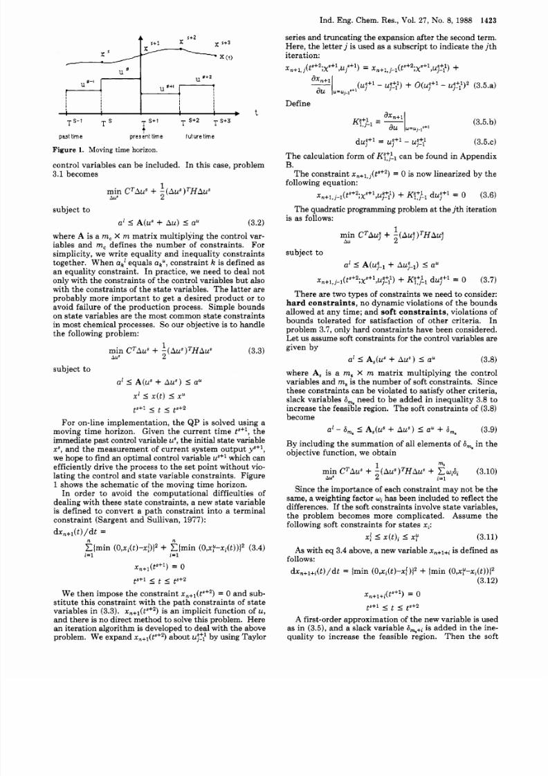
Figure 1. Moving time horizon.

control variables can be included. In this case, problem

3.1 becomes

I

min

CTAus

+ - ( A u ~ ) ~ H A u ~

ub

2

subject to

al

I

A(us + Au) (3.2)

where A is a

m,

X

m

matrix multiplying the control var-

iables and

m,

defines the numb er of constrain ts. For

simplicity, we write equality and inequality constraints

together. When

ahL

quals

abu,

constraint

k

is defined as

an equality constraint. In practice, we need to deal not

only with the con straints of the control variables bu t also

with the constraints of the stat e variables. Th e latter are

probably more important to get a desired product or to

avoid failure of th e production process. Sim ple bound s

on s ta te variables are th e most common state constraints

in most chemical processes. So our objective is to hand le

the following problem :

1

hU8 2

in CTAuS+ - ( A u ~ ) ~ H A u ~ (3.3)

subject to

a1

(us

+

Aus)

X I ( t )

I

u

tS+1 5 I s + 2

For on-line implementation, the QP is solved using a

moving time horizon. Given the current t ime ts+l, the

imm ediate past control variable

us,

he initial sta te variable

x s ,

and th e measurement of current system outp ut yS+l,

we hope to find

an

optim al control variable uS +lwhich can

efficiently drive th e process to the set point w ithout vio-

lating the control and s ta te variable constraints . Figure

1

shows the schematic of the moving time horizon.

In order to avoid the computational difficulties of

dealing with these s ta te constraints , a new sta te variable

is defined to convert a path constraint into a terminal

constraint (Sargent and Sullivan, 1977):

d x n + l ( t ) /d t

=

n n

i = l i = l

C ( m i n ( o , ~ ~ ( t ) - x f ) ) ~E l m i n

( o , x y - ~ ~ ( t ) ) ) ~

3.4)

X , + l ( t s + l ) = 0

p+ l 5 S + 2

W e t he n im pose t he constraint ~ , + ~ ( t ~ + ~ )

0

and sub-

sti tu te this constraint with the path constraints of s tat e

variables in (3.3). ~ , + ~ ( t ~ + ~ )s an implicit func tion of u,

and there is no direct method to solve this problem. Here

an iteration algorithm is developed to deal with th e above

problem. We expan d x, +, (P 2) about u;?; by using Taylor

Define

(3.5.b)

duS++l

= u B + l

u4+1-1 (3.5.c)

Th e calculation form of K _, can be found in Appendix

B.

The constraint x , + ~ ,

( t s + 2 )

= 0 is now linearized by the

following equation:

xn+l, - l( ts+2;~s+ 1,~;?l)K L1 dug+' = 0

(3.6)

The quadratic programming problem at th e jt h iteration

is as follows:

1

min CTA$

+

- ( A u ; ) ~ H A u ~

Au

2

subject to

There a re two types of cons traints we need t o consider:

hard constraints,

no dynam ic violations of the bounds

allowed a t any time; and soft constraints, violations of

bound s tolerated for satisfaction of other criteria. In

problem 3.7, only hard c onstraints have been considered.

Let us as sume soft constraints for the control variables are

given by

(3.8)

where A, is a m,

X

m matrix multiplying the control

variables and m, is th e number of soft constraints. Since

these constraints can be violated to satisfy other criteria,

slack variables am need to be added in inequality 3.8 to

increase th e feasible region. Th e soft cons traints of (3.8)

become

(3.9)

in the

ul

s(us

+

Aus)

U' 1 3 , ~ s(uS

+ ALP )

+

By including the s umm ation of all elements of

objective function, we obtain

m.

min CTAus

+

. t ( A ~ s ) T H A ~ s

c w i 6 i

(3.10)

A 8 2 i= l

Since the importance of each constraint m ay not be th e

same, a weighting factor

wi

has be en included

to

reflect the

differences. If the soft constraints involve st ate variables,

the problem becomes more complicated. Assume the

following soft constraints for states

xi:

(3.11)

As with eq 3.4 above, a new variable

x , + ~ + ~

s defined as

x j

( t ) ;

y

follows:

dx,+l+i(t)/dt = (min ( O , x i ( t ) - ~ f ) ] ~ (min ( o , ~ Y - x ~ ( t ) ) ) ~

(3.12)

Xn+l+i(ts+l)= 0

ts+l 5

t

s + 2

A first-order approx imati on of the new variable is used

as in (3.5), an d a slack variable

~5+~

is added in the ine-

quality to increase the feasible region. Th en the soft



1424


27,

No.

8,

1988

constrain t of (3.11) in the jt h iteration now becomes

x,+l+i, j - l t s + 2 ; x s + 1 , ~ ~ ? ~ )Kjzi, -1 duS+' m,+i

(3.13)

T h e vector form of these constra ints (with dimension

m,)

U

7

(3.14)

du; (3.15)

r e d u c e s t e p s i z e

axn+l+i

Ka+l

+ i , j u

Iu=u,.l~ l i

= 1, 2, 3, ..., m,

Including soft constraints 3.14, the quadra tic program-

ming problem a t the j t h i teration now becomes

mt

AUS

2 i=

1

1

min

CTAus +

- ( A u ~ ) ~ H A u Y

2 ~ ~ 6

3.16)

subject to

ul

(U;-~

+

Aus-,)

5

u

6mB

,(uj-,

+

Auj-1)

+

6m8

Nj(tS+2;XS+1,ujS?i)mx

L

0

where

m,

=

m,

+

m,

is the total number of all soft con-

s t ra in ts .

Finally, it is worth noting that before the hard s tate

constraints are included in the control algorithm, the

feasibility of these state constraints has to be analyzed.

Even though t he hard sta te constraints are feasible in the

model, the system states can easily be pushed o ut from the

feasible region by the disturbances in the real process.

Therefore, it is recommended to tr eat all stat e constraints

as soft constraints .

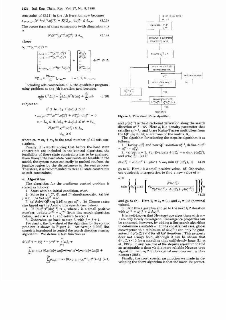
4. Algorithm

stated as follows:

The algorithm for the nonlinear control problem is

1. St art w ith an init ial condition,

xs,us.

2. Solve for xs ,

Cs,

P n d rs imultaneously. (a) Se t

j =

0.

( b ) Se t u$+' =

us.

3. (a)Solve Q P (eq 3.16) to get (b) Choose a step

size based on the Armijo line search (see below).

4. If (du;+ ')T(du s+l)

<

E where t is a small positive

number, update

us++=

us+'

(from line search algorithm

below), set s = s

+

1, and re turn to s tep 1.

5 . Otherwise, go back to s tep 3, with j = j + 1.

For clarity, the flow shee t of the algorithm for the control

problem is shown in Figure 2. An Armijo (1966) line

search is introduced to control the search direction stepsize

algorithm. We define a test function as

mt

(ug+l) =

(y;+2 y*)2 +

C W J i +

i=l

ma

i=l

c p i max ~O , ~~( u ~+ A u ~) - 6 ~ - u . , a - a ~ - u ~( u ~+ ~u ~) }

m

r=l

C P m s + i max

{O,xn+l+i,( X s + ' , U ~ + ' ) - 6 i I

(4.1)

1

g i v e n i i i t i a l c o n d

ca lcu la te r',o'

1. Having us-: an d new QP solution us+', define dug+'

-

us+l

us+l

.-, .

2.

(a)

Sgia

= 1. (b) Evaluate $(u;?:

+

a d u ) ,

$(uj?t),

and $'(u;?:). (c) If

$(ug?f

+

a dug ) $(us )

I

h1

min (+ (u;?:),-E) (4.2)

go to 3. Here

E

is a small positive value.

(d) Otherwise,

use quadratic interpolation to find a new value of a

(4.3)

and go to (b) . Here

61

=

1 3 ~

0.1 an d 6, = 0.8 (nominal

values).

3. Exit this algorithm and go to the next Q P iteration

with us

=

us-:' + a du; .

It

is well-known that Newton-type algorithms with

a =

1 are only locally convergent. Convergence propertie s can

be enhan ced, however, by adding a line search algorithm

to determine a suitable a. In t he constrained case, global

convergence to

a

minimum of

$(uj f l )

an only be guar-

ante ed if +'(uJ?l)<

0

for all Q P iterations. This property

does not always hold, although i t can be shown that

' (uJ?l)< O for a sampling time sufficiently large (Li et

al., 1988). In any case, use of the stepsize algorithm to find

an acceptable a does yield a more reliable New ton-type

algorithm th an eq 2.6, th e original one proposed by Eco-

nomou (1985).

Finally, the most crucial assumption we made in de-

veloping the above algorithm is th at th e model be perfect.



Ind. Eng. C hem. Re s., Vol. 27, No. 8, 1988

1425

Table I. Parameter Values of Example 1

uarame ter Darameter set Doint

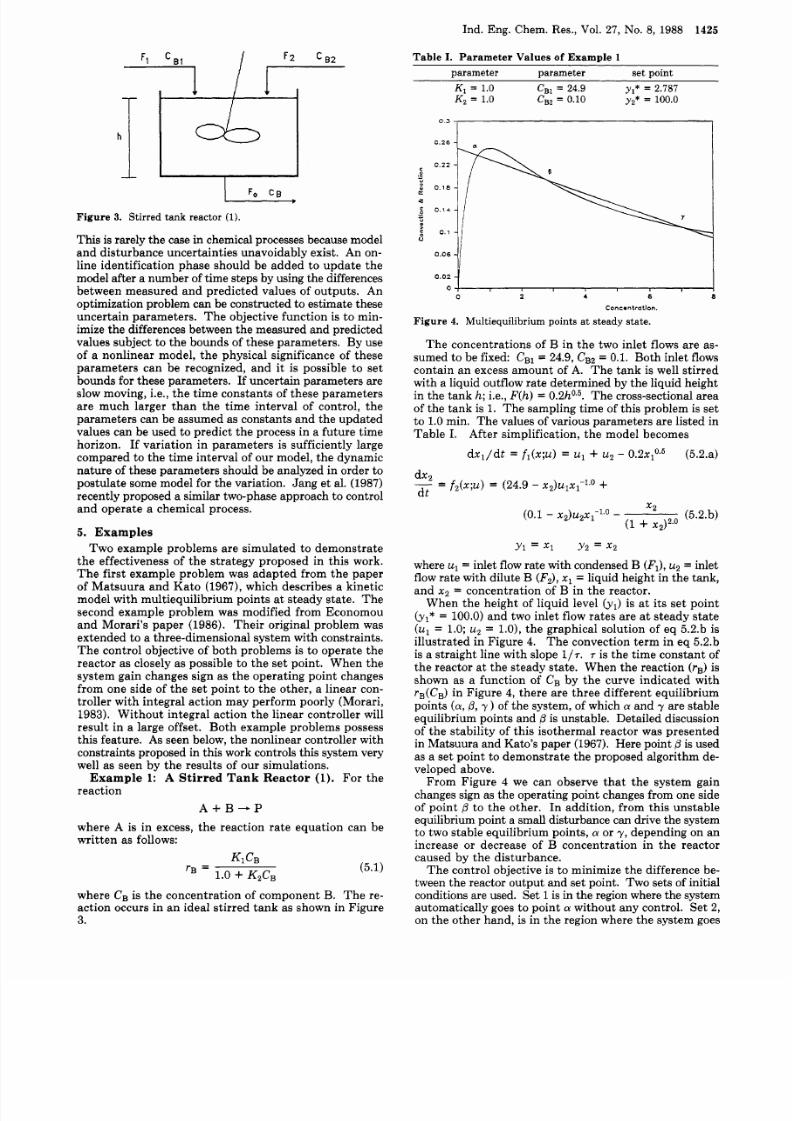
Figure

3.

Stirred tank reactor (1).

This is rarely th e case in chem ical processes because model

and disturbance u ncertainties unavoidably exist. An on-

line identification phase should be added to u pdate t he

model after a num ber of time steps by using the differences

between measured an d predicted values of outputs. An

optimization problem can be constructed to estimate these

uncertain parameters . Th e objective function is to min-

imize the differences between the measured a nd predicted

values subject to the bounds of these parameters. By use

of a nonlinear model, the physical significance of these

parameters can be recognized, and it is possible to set

bounds for these parameters. If uncertain param eters are

slow moving, i.e., th e tim e constan ts of these p aram eters

are much larger than the t ime interval of control, the

parameters can be assumed as constants and th e updated

values can be used to predict th e process in a future time

horizon. If variation in para me ters is sufficiently large

compared t o the time interval of our model, the dynamic

nature of these param eters should be analyzed in order to

postulate some model for the variation. Jang et al. (1987)

recently proposed a similar two-phase approach to control

and operate a chemical process.

5. Examples

Two example problems are s imulated to dem onstrate

the effectiveness of the strategy proposed in this work.

T he f irs t example problem was adapted from the paper

of M atsu ura an d K at0 (1967), which describes a kinetic

model with multiequilibrium points a t s teady s tate. Th e

second example problem was modified from Economou

and Morari's paper (1986). Their original problem was

extended to a three-dimensional system with constraints.

Th e control objective of both problem s is to operate th e

reactor as closely as possible to the se t point. Wh en the

system gain changes sign as the operating point changes

from one side of th e set point t o the o ther, a linear con-

troller with integral action may perform poorly (Morari,

1983). W ithou t integral action the linear controller will

result in a large offset. Both exam ple problems possess

this feature . As seen below, th e nonlinear controller with

constraints proposed in this work controls this system very

well as seen by t he results of our sim ulations.

Example 1:

A

Stirred Tank Reactor ( 1 ) . For the

reaction

A + B - P

where A is in excess, the reaction rate equation can be

written as follows:

(5.1)

where C B is the concentration of compone nt B. Th e re-

action occurs in an ideal stirred t ank as shown in Figure

3.

0 26

0 . 22

0

-

5

0 .18

C

a

0 16

-

>

U

0 . 1

0 02

06

4 I

0 7 4 6

8

Ccnc.ntrctlon.

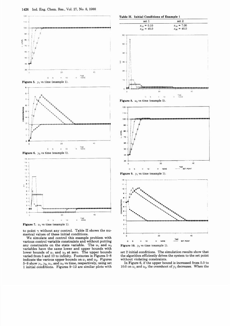
Figure 4. Multiequilibrium points at steady state.

Th e concentrations of B in th e two inlet flows are as-

sumed to be fixed: cB1 = 24.9, CB, = 0.1. Both inlet flows

contain an excess am oun t of A. Th e tank is well stirred

with a liquid outflow rate determined by the liquid height

in the tank

h;

.e.,

F ( h )

= 0.2h0.5.Th e cross-sectional area

of th e tank is 1. The sampling time of this problem is set

to 1.0 min. Th e values of various parame ters are listed in

Table I. After simplification, the model becomes

d x l / d t = fl(x;u) u1 +

u2

0 . 2 ~ , ~ . ~

5.2.a)

X P

(0.1 x 2 ) u 2 x 1 - ~ ~ o

(5.2.b)

(1+

x p

Y1

=

x1 Y2

=

x2

where

u1

=

inlet flow rate with condensed B

( F J ,

u2

=

inlet

flow rate w ith dilute

B

(F2) , 1

=

liquid height in th e tank,

an d x 2

=

concentration of B in the reactor.

When the height of liquid level (yl) is at i ts set point

yl* = 100.0)and two inlet flow rates are a t s teady s tate

(ul = 1.0; u2 = 1.01, th e grap hical s olution of eq 5.2.b is

illustrated in Figure 4. Th e convection term in eq 5.2.b

is a straight line with slope 1 / ~ . s the ti me consta nt of

th e reactor at the steady state. When th e reaction (rB) s

shown as a function of CB by the curve indicated with

r B ( C B )

in Figure 4, here are three different equilibrium

points (a ,p, y ) of th e system, of which a an d y are stable

equilibrium points and p is unstable. Detailed discussion

of the stability of this isothermal reactor was presented

in Matsuura an d Kato's paper (1967). H ere point

/3

is used

as a set point to demons trate t he proposed algorithm de-

veloped above.

From Figure

4

we can observe that the system gain

changes sign as the operating point changes from one side

of point p to the other. In addition, from this unstable

equilibrium point a small disturbance can drive the system

to two stable equilibrium points, a or y, depending on an

increase or decrease of B concentration in the reactor

caused by the disturbance.

Th e control objective is to minimize th e difference be-

tween the reactor outpu t and set point. Two sets of initial

conditions are used. Set

1

s in the region where the system

automatically goes to point

a

without any control. Set 2,

on the other ha nd, is in th e region where the system goes



1426 Ind. E ng. C hem. Res., Vol. 27,

No.

8, 1988

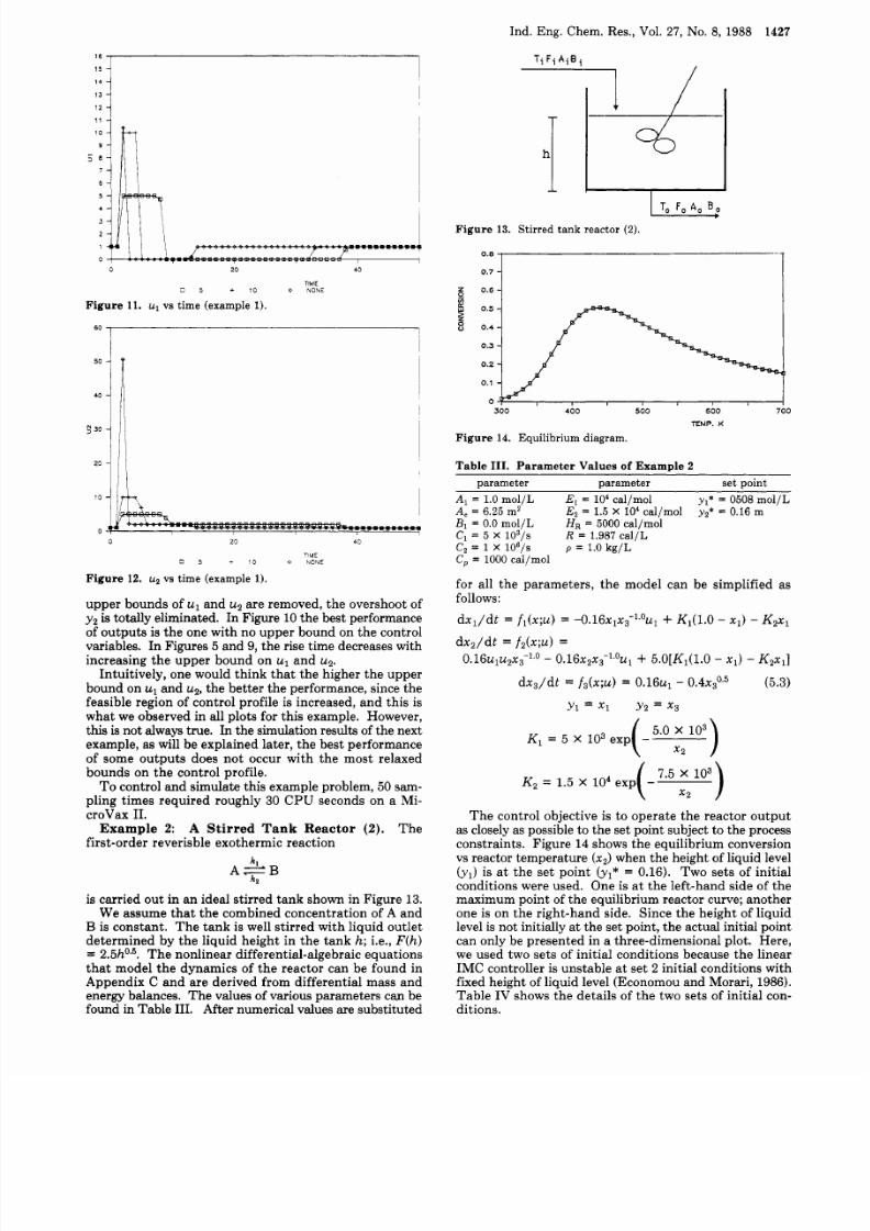
15 __ _ ~ ~ -

14 -

1

5 2

1

1

100

01 _ _ _ _ _ ~_ ~ 4

23 4s

ME

0 5 - 10 h O NE

Figure 5. y1 vs time (example 1).

Table 11. I nitial Conditions

of

Example

set 1 set 2

nlo

= 0.10 = 7.00

xzo = 40.0

~ 2 0

40.0

0

2c

4:

TIIIE

5

5

10 0 P.0'E

Figure 8. uz vs time (example 1).

120 I

3

.

70

60

500

Y

30 I 1

0

20 40

l l M E

0 5 + 1 0

NONE

__

SET

POINT

Figure 9. y1

vs

time (example 1).

:

20

40

TIME

SET

POINT

--

5

+ 1 0

NONE

Figure 10 y2 s

time (example 1).

set

2

initial conditions. T he simulation results show tha t

the algorithm efficiently drives the system to th e se t point

without violating constraints.

In Figure

6,

if the upper bound is increased from

5.0

t o

10.0 on u1and u2, he overshoot of yzdecreases. When the




1427

4 0 -

2 3 0 -

15

14

13

11

12

10

9

s

7

6

5

4

3

2

1

0

0

20

40

TIME

0 5

+ 1 0 NONE

F i g u r e 11 u1

vs

t ime (example 1).

-- ~

10

0

0

20

40

1ME

0 5 + 10

NONE

F i g u r e

12.

u 2

vs

t ime (example 1).

upper bounds of u1 and

u2

are removed, the overshoot of

yz

s totally eliminated. In Figure 10 the best performance

of ou tpu ts is th e one with no upper bound on th e control

variables. In Figures 5 and 9, the rise time decreases with

increasing the upper bound on u1 an d uz.

Intuitively, one would think that the higher the upper

bound on u1and u2, he bette r th e performance, since the

feasible region of control profile is increased, and thi s is

wha t we observed in all plots for this exam ple. However,

this is not always true. In th e simulation results of the next

example, as will be explained la ter, th e best performance

of some outputs does not occur with the most relaxed

bounds on the control profile.

To control and sim ulate this example problem, 50 sam-

pling times required roughly 30

CPU

seconds on a Mi-

croVax 11.

Example

2:

A

Stirred Tank Reactor

(2).

T h e

first-order reverisble exotherm ic reaction

k

kz

A + B

is carried ou t in an ideal stirred tan k shown in Figure 13.

We assume that the combined concentration of A an d

B

is consta nt. Th e tank is well stirred with liquid outlet

determin ed by the l iquid height in the tan k h; i.e., F(h)

= 2.5h0.6.Th e nonlinear differential-algebraic equations

that model the dynamics of the reactor can be found in

Appendix C and are derived from differential mass and

energy balances. T he values of various param eters cap be

found in Table 111. After numerical values are substitu ted

F i g u r e

13.

Stirred tank reactor (2).

0 7

1

0 6 1

TEMP. K

F i g u r e 14. Equilibrium diagram.

T a b l e 111. P a r a m e t e r V a l ue s of ExamDle 2

parameter parameter set point

E,

=

lo4

cal/mol y l * = 0508 mo l/L

E ,

= 1.5 X l o4 cal/mol yz* = 0.16 m

H R

=

5000 cal/mol

R = 1.987 cal/L

p

= 1.0

kg / L

A,

=

1.0 mol/L

A, =

6.25 m2

B1 =

0.0

mol/L

C, = 5 X 103/s

C, = 1 X 106/s

C = 1000 cal/mol

for all the parameters, the model can be simplified as

follows:

d x l / d t

=

f l ( x ; u )

=

-0.16x1x3-1.0u1

+

K1 l.O

xl)

Kzxl

d x , /d t = f z ( x ; u )=

0.16u1u2x3-1.0 O.l6 ~2 x3-~ .~u 15.O[K1(1.0

X I )

Kzxl]

d x 3 /d t = f3(x;u) = 0 .1 6 4 0 .4 x ~O.~

(5.3)

Y1 =

x 1

Y z

=

x3

5.0

x

103

Kl

= 5 x

103

exp(- x z )

7.5

x

103

K z =

1.5 X lo4ex.( x z )

Th e control objective is to operate the reactor o utp ut

as closely as possible to the set point su bject to th e process

constraints. Figure 14 shows the equilibrium conversion

vs reactor temperature xz)when th e height of liquid level

(yl) s a t the se t po int (yl* = 0.16). Two sets of initial

conditions were used. One is at th e left-hand side of t h e

maximum point of the equilibrium reactor curve; another

one is on th e right-hand side. Since the height of liquid

level is not initially at the set point, th e actua l initial point

can only be presented in a three-dimensional plot. Here,

we used two sets of initial conditions because the linear

IMC controller is unstable a t set

2

initial conditions with

fixed height of liquid level (Econom ou and M orari, 1986).

Table IV shows the details of th e two sets of initial con-

ditions.



1428 Ind. Eng. Chem. Res., Vol. 27, No. 8,

1988

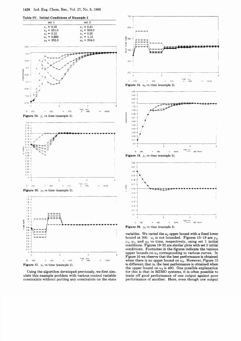
Table IV. Initial Conditions

of

Example 2

set 1 set 2

x 1 = 0.16 x l = 0.41

~2 = 351.0 X Z

= 503.0

x g

=

0.12

ul

= 0.866

X 3

=

0.20

u1

=

1.12

up = 352.0

~2

=

504.0

2 5

'3

' 5

0 4

2

c

0 35

z

C 3

0 2 5 - b

8

a

2 4

6

TIME

min

3 433 f 450 0

470

A 490 X NONE

Figure 15.

y l

vs time (example 2).

2 4

-1ME m n

c

13:

- 153 0 470 3

490

Figure 16.

y 2


5

X

UCUE

I

0 -

I

2

4

6

1ME

m i

0 430 +

450

d70

n 493

X

?ONE

Figure 17. u1

vs

time (example 2).

Using the algorithm de veloped previously, we first sim-

ulate this example problem w ith various control variable

constraints without putting any constraints on the s t ate

1

3 0 c -

1 -

ci ~-

2 L 6

TME 7 1 , ~

c

433 +

450

0 473 A

4g3

X U31E

Figure 18.

u2 s

time (example 2).

3

54

c 5 5

i

0 5 2

-

I

0 44

I

I

I

0 4 I

0 2 4 6

ME min

SET POIhT

430

i

450 0 NONE

Figure 19. y 1 vs time (example 2).

2

0 2 2

::h-

8

7

0

16

3 - 5i

: I

I

0 12

0 1 1

--

___

l

0 2 4

6

TIME

m r

0 UOYE

F

POINT

430 t

455

Figure 20. yz

vs

time (example 2).

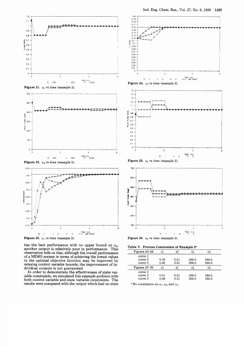
variables. We varied the

up

pper bound with a fixed lower

bound a t 300. u1 is not bounded. Figures 15-18 are

yl,

y2, ul , and u2 vs time, respectively, using set 1 initial

conditions. Figures 19-22 are similar plots with set 2 initial

conditions. Footnotes in the figures indicate the various

upper bounds on u2corresponding to various curves. In

Figure 16 we observe th at t he best performance is obtained

when there is no upper bound on u2. However, Figure 15

is different; th at is, the best perform ance is obtained when

the upper bound on u2 s 490. One possible explanation

for this is tha t in MIMO systems, i t is often possible to

trade off good performance of one output against poor

performance of another. Here, even though one out put




27,

No.

8, 1988

1429

1 2

1 1

1

09

08

0 4 i

0 3

-

1:

o

0

2 4

6

TIME m n

C

430

- 450 NOhE

Figure 21. u1 vs time (example 2).

__

600

,

I

00

1

0

2 4 6

TIME

min

0 430 + 450

NONE

Figure 22. u 2 vs time (example 2).

0 55

I

_.

0

2 4 6

TIME

min

SET

POINT

1

+ 2

0 3

Figure

23. y1


has the best performance with no upper bound on u2,

anoth er outpu t is relatively poor in performance. Th is

observation tells us tha t, although th e overall performance

of a MIMO system in term s of achieving the lowest values

in the optimal objective function may be improved by

relaxing control variable bounds, the improvement of in-

dividual outputs is not guaranteed.

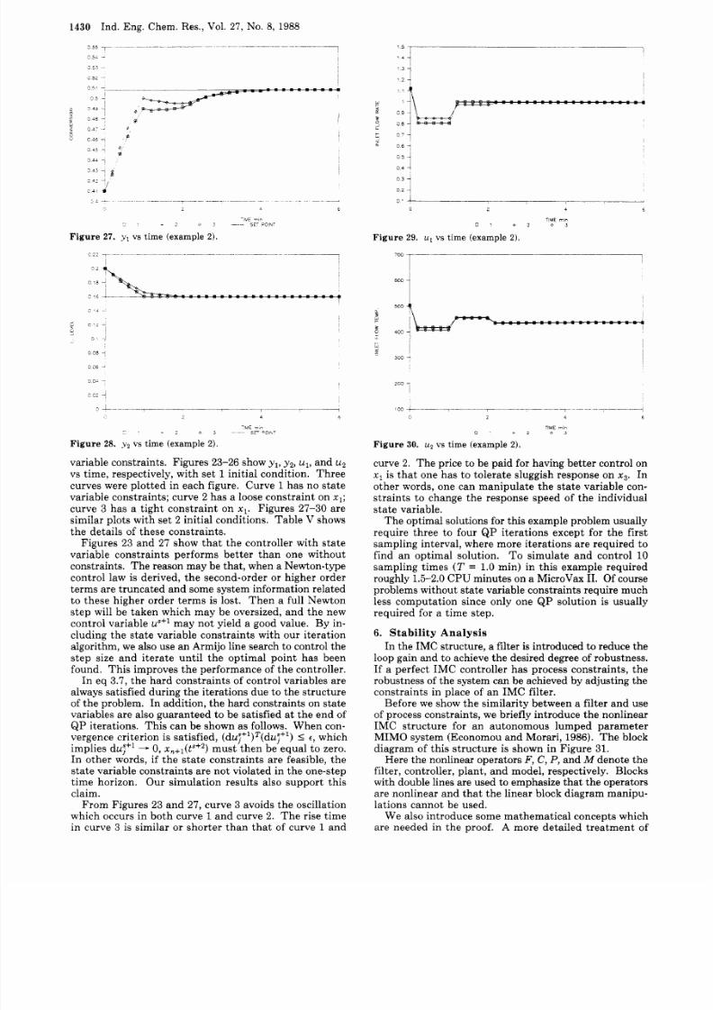
In order to dem onst rate the effectiveness of sta te var-

iable constraints, we simu lated this example problem w ith

both control variable and state variable constraints. Th e

results were compared with the outpu t which had no state

0 .16

0 . 1 5

0.14

0.13

0.12

4 0.11

0

07

0 0 6 4

Y

0 5

4

I

:::

0 02

0

01

0 ,

0

2 4 6

nME min

0 1 + 2

0 3 - SET POINT

Figure 24. y2 vs time (example 2).

0

0

2

4

TIME

min

0 1 2

0 3


6

700

I

1 I

200I

TIME

min

n i + 2 0 3


Table V. Process Constraints

of

Example 2

Figures 23-26 xi x ;

2:

X :

curve

1

curve 2 0.16 0.51 300.0 550.0

curve 3 0.40 0.51 300.0 550.0

Figures 27-30

2:

x : 2:

x ;

curve

1

curve 2 0 .41 0.51 300.0 550.0

curve 3 0.49

0.51

300.0

550.0

N o constraints on ul, u2,and x g .



1430


27, No.

8, 1988

0 s ' -

1 5 3

i ' 5 i

.

- M E

T II

* * J S T OINT

. .

Figure

27.

y1

vs t ime (example 2).

008

0 0 6

3 0 - -

I

sc; -1

r

_

-. ___

4

- M E

m n

- 2

e , ~ 5 7 Olh-

Figure 28.

y 2

vs

t ime (example 2).

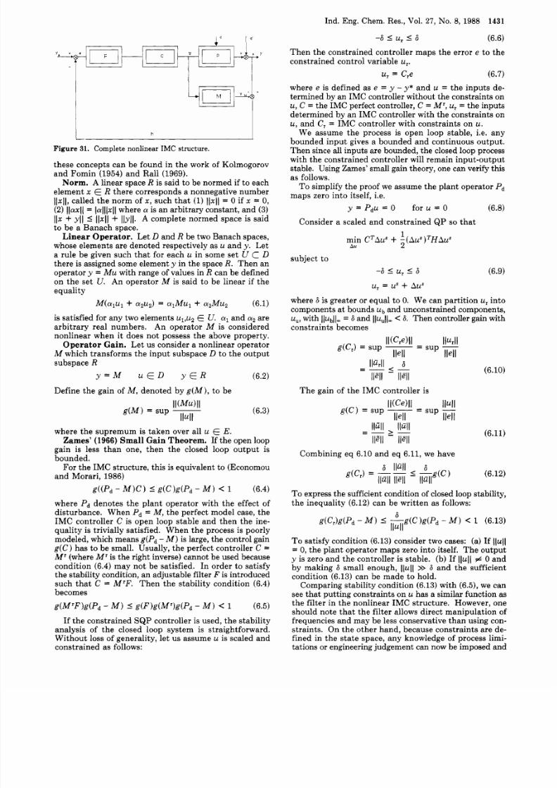
variable constraints. Figures 23-26 show

yl,

y 2 ,

ul,

nd

u2

vs time, respectively, with set 1 initial condition. Thr ee

curves were plotted in each figure. Curve 1has no s ta te

variable constraints; curve 2 has a loose constraint on xl;

curve 3 has a t ight constraint on

q

igures 27-30 are

similar plots with set 2 initial conditions. Table

V

shows

the details of these constraints.

Figures 23 and 27 show tha t the controller with s tate

variable constraints performs better than one without

constraints. Th e reason m ay be that, when a Newton-type

control law is derived, the second-order or higher order

terms are truncated and some system information related

to these higher order terms is lost . Th en a full Newton

step will be taken which may be oversized, and the new

control variable uS lmay no t yield a good value. By in-

cluding the s tat e variable constraints with our i teration

algorithm, we

also

use an Armijo line search to control the

step s ize and iterate until the optimal point has been

found. Th is improves th e performance of the controller.

In eq

3 .7 ,

the hard constraints

of

control variables are

always satisfied during the iterations d ue to the structure

of the problem. In addition, the hard con straints on state

variables ar e also guaranteed to be satisfied at th e e nd of

QP iterations. Thi s can be shown as follows. Wh en con-

vergence criterion is satisfied, (du;+l)T(duy+l)

5

, which

imp lies du; -

,

~ , + ~ ( t ~ + ~ )ust then be equal to zero.

In o ther words, if th e s tate constraints a re feasible, the

sta te variable constraints are not violated in th e one-step

time horizon. Our simulation results also supp ort this

claim.

From Figures 23 an d 27, curve 3 avoids the oscillation

which occurs in both curve

1

and curve 2. Th e r ise t ime

in curve 3 is similar or shorter than that of curve 1 an d

Figure 29.

u1

vs

time (example

2) .

I

600

~ _ _ _

._

_

0 c

0 2 4 6

TIME

m / n

0

c 2 e 3

Figure 30. upvs

time (example 2) .

curve 2. Th e price to be paid for having be tter control on

n, is tha t one has to tolerate s luggish response on x 3 . In

other words, one can m anipulate th e s tate variable con-

straints to change the response speed of the individual

state variable.

Th e optimal solutions for this exam ple problem usually

require three to four QP iterations except for the f irs t

sampling interval, where more iterations are required to

find an optimal solution. To s imulate and control 10

sampling times

(T

= 1.0 min) in this example required

roughly 1.5-2.0 CP U minu tes on a M icroVax 11. Of course

problems without sta te variable constraints require much

less computation since only one QP solution is usually

required for a time s te p.

6 . St a b i li t y Ana ly s i s

In the IMC s tructure, a filter is introduced to reduce the

loop gain and to achieve the d esired degree of robustness.

If a perfect IMC controller has process constraints, the

robustness of the system can be achieved by adju sting the

constraints in place of an IMC filter.

Before we show the similarity between a filter and use

of process co nstrain ts, we briefly introdu ce th e nonlinear

IMC structure for an autonomous lumped parameter

MIM O system (Economou and Morari, 1986). The block

diagram of this struc ture is shown in Figure 31.

Here the nonlinear operators

F ,

C,

P,

and M denote the

filter, controller, pla nt, and m odel, respectively. Blocks

with double lines are used to emphasize th at th e operators

are nonlinear an d tha t the linear block diagram manipu-

lations cannot be used.

We also introduce some mathematical concepts which

are needed in the proof. A more detailed treatme nt of



i d I d


1431

-6 ,

(6.6)

Th en the constrained controller maps th e error e t o th e

constrained control variable

u,.

u ,

=

C,e (6.7)

where e is defined as e = y - y* an d

u

= the inputs de-

termined by an IMC controller without the constraints on

u, C

=

the IMC perfect controller, C =

M I , u ,

= the inputs

determined by an IMC controller with the co nstraints on

u , and C,

=

IMC controller with constraints on u .

We assume the process is open loop stable, i.e. any

bounded inpu t gives a bounded and continuous output.

Th en since all inputs are boun ded, the closed loop process

with the constrained controller will remain input-output

stable. Using Zames' small gain theory, one can verify this

as follows.

To simplify the proof we assume th e plant operator pd

maps zero into itself, i.e.

y =

Pdu

= 0 for u

=

0 (6.8)

Consider a scaled and constrained QP so t h a t

1

Au

2

in CTAus

+

- ( A u ~ ) ~ H A u ~

subject to

-6 ,

u, = us+

Aus

where

6

is greater or equal to 0. We can partition

u ,

into

components at bounds ub and unconstrained com ponents,

uu,with

IIub(lm

= 6 and

IJu,J(,

< 6. The n controller gain with

constrain ts becomes

(6.9)

I

G e )

I Ilurll

g(C,)

=

sup ~

=

s u p

l lell l lell

h

Figure

31. Complete nonlinear

IMC

structure.

these concepts can be found i n the work of Kolmogorov

and Fomin (1954) and Rall (1969).

Norm.

A linear space R s said to be normed if to each

element x

E

R there corresponds a nonnegative number

IIxII called the norm of x , s u ch th a t

(1)

11x11 =

0

if x =

0,

(2) ((axil

= Iall lxl l

where a is an arbitra ry constant, and (3)

I I x + yIJ 1x11 + Ilyll. A complete normed space is said

to be a Banach space.

Linear Operator. Let

D

and R be two Banach spaces,

whose elements are den oted respectively as

u

and y. Let

a rule be given such th at for each

u

in some set

U D

there is assigned some element

y

in the space

R.

Then an

operator

y =

M u with range of values in R can be defined

on the se t U . An operator

M

is said to be linear if the

equality

M(a1U1

+ C Y ~ U ~ )

( Y ~ M u ~C XZM U~

(6.1)

is satisfied for any two elements

u1,u2

E

U . a1 nd

a 2

are

arbitrary real numbers . An operator M is considered

nonlinear when it does not possess the above property.

Operator Gain. Le t us consider a nonlinear operator

M which transforms th e input subspace D t o th e o u tp u t

subspace R

y = M

u E D

y E R (6.2)

Define t he gain of M , denoted by g ( M ) , o be

(6.3)

where the su premum is taken over all

u

E E .

Zames (1966) Small Gain Theorem.

If the op en loop

gain is less than one, then the closed loop output is

bounded.

For th e IM C structu re, this is equivalent to (Economou

and Morari , 1986)

g ( (p d M ) C ) ( c ) g ( p d M I < 1 (6.4)

where

Pd

denotes the plant operator with the effect of

dis turbance. When Pd

=

M , the perfect model case, the

IMC controller C is open loop s table and then the ine-

quality is trivially satisfied. Wh en th e process is poorly

modeled, which means g(pd

M )

s large, the control gain

g ( C )

has to be small. Usually, the perfect controller C =

MI

(where

M '

is the right inverse) cann ot be used because

condition (6.4) may n ot be satisf ied. In order to satisfy

the stability condition, an adjustable filter F is introduced

such tha t

C = M 'F.

Th en th e s tabili ty condition (6.4)

becomes

g ( M ' F ) d P d

-

M ) ( F )g (M ') d Pd M )

<

1 (6.5)

If the constrained SQP controller is used, the s tability

analysis of the closed loop system is straightforward.

Wi thou t loss of generality, let us assum e u is scaled and

constrain ed a s follows:

T he gain of th e IMC c ontroller is

(6.10)

(6.11)

Combining eq 6.10 and eq 6.11, we have

(6.12)

l l a l l 6

ll4l ~ lFll

(C,)

= g (C)

T o express the sufficient condition of closed loop stability,

the inequality (6.12) can be w ritten as follows:

To satisfy condition (6.13) consider two cases: (a) If

llull

=

0, the plant operator maps zero into itself. T he outpu t

y is zero an d the co ntroller is stable. (b) If

llull

0 an d

by making 6 small enough,

llull

>>

6 and the sufficient

condition (6.13) can be made to hold.

Com paring stab ility con dition (6.13) with (6.5), we can

see tha t putting constraints on

u

has a similar function as

the f i l ter in the nonlinear IMC structure. However, one

should note that the filter allows direct manipulation of

frequencies an d m ay be less conservative tha n using con-

straints . On the other hand, because constraints are de-

fined in th e st ate space, any know ledge of process limi-

tations or engineering judge men t can now be imposed an d



1432

Ind. Eng. C hem. Res., Vol.

27, No. 8, 1988

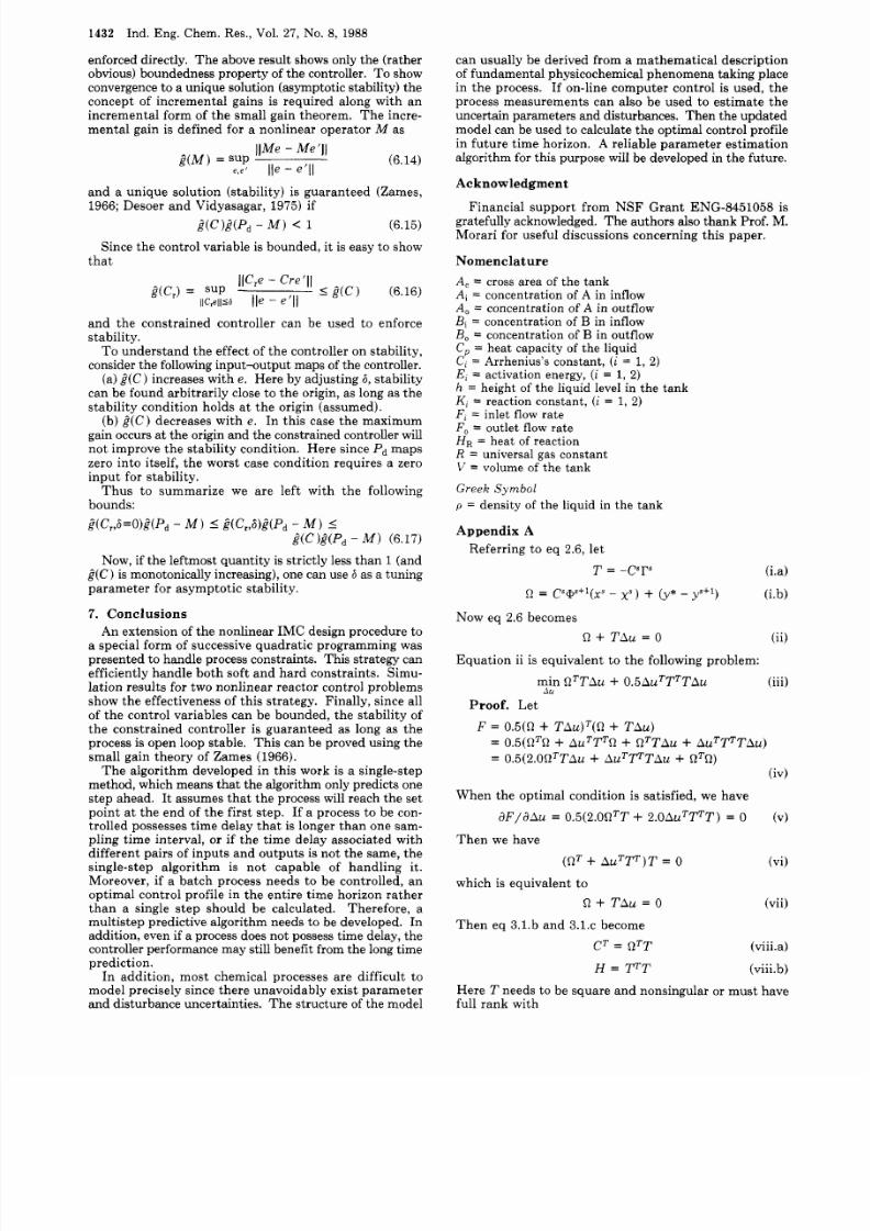
enforced directly. Th e above result shows only the (rath er

obvious) boundedness property of the controller. T o show

convergence to a unique solution (asymptotic stability) the

concept of incremental gains is required along with an

incremental form of the small gain theorem. Th e incre-

mental gain

is

defined for a nonlinear ope rator

M

as

and a unique solution (stability) is guaranteed (Zames,

1966;

Desoer an d Vidyasagar,

1975)

if

d ( C ) i ( p d M ) < 1 (6.15)

Since the c ontrol variable is bounded , it is easy to show

t h a t

and the constrained controller can be used to enforce

stability.

To

unde rstand the effect of the controller on stability,

consider the following inpu t-ou tpu t maps of th e controller.

(a) d ( C ) ncreases with e . Here by adjusting 6, stability

can be found arbitrarily close to t he origin, as long as the

stability condition holds a t the origin (assumed).

(b)

i ( C )

decreases with

e.

In this case the maximum

gain occurs at the origin an d th e constrained controller will

not improve the stability condition. Here since p d maps

zero into itself, the w orst case condition requires a zero

input for stability.

Thus to summarize we are left with the following

bounds:

Now, if the leftmost q uan tity is strictly less than 1 (and

i ( C ) s monotonically increasing ), one can use

6

as a tuning

parameter for asy mptotic s tability.

7.

Conclusions

An extension of the n onlinear IM C design procedure to

a special form of successive quadratic programming was

presented to handle process constraints. This strategy can

efficiently handle both soft an d hard constraints . Simu-

lation results for two nonlinear reactor control problems

show the effectiveness of thi s strategy. Finally, since all

of the con trol variables can be b ounded, t he s tability of

th e constrained controller is guaranteed as long as the

process is open loop stable. Th is can be proved using the

small gain theory of Zames

(1966).

T he algorithm developed in th is work is a single-step

method, which means th at th e algorithm only predicts one

ste p ahead. It assumes tha t the process will reach the set

point a t the end of the first step. If a process to be con-

trolled possesses time delay th at is longer tha n o ne Sam-

pling time interval, or if th e tim e delay associated w ith

different pairs of input s and outpu ts is not the same, the

single-step algorithm is not capable of handling it.

Moreover, if a batch process needs to be controlled, an

optim al control profile in the e ntire time horizon rather

th an

a

single step should be calculated. Therefore, a

mu ltiste p predictive algorithm needs to be developed. In

add ition , even if a process does no t possess time delay, the

controller performance may still benefit from th e long time

prediction.

In addition, most chemical processes are difficult to

model precisely since the re unavoidably exist param eter

and disturbance uncertainties. Th e structur e of the model

can usually be derived from a mathematical description

of funda me ntal physicochemical pheno men a takin g place

in th e process. If on-line computer control is used, the

process measurements can also be used to estimate the

uncertain parameters and disturbances. Th en the updated

model can be used t o calculate th e optimal control profile

in future time horizon. A reliable param eter estimation

algorithm for this purpose will be developed in the future .

Acknowledgment

Financial support from

NSF

Grant

ENG-8451058

is

gratefully acknowledged. T he auth ors also tha nk Prof. M.

Mora ri for useful discussions concerning this paper.

Nomenclature

A, = cross area of the tank

A i = concentration

of A

in inflow

A,

=

concentration

of A

in outflow

Bi

= concentration of

B

in inflow

B , =

concentration

of

B in outflow

C

= heat capacity of the liquid

C, =

Arrhenius’s constan t, i = 1, 2)

E , =

activation energy, i =

1,

2)

h

=

height

of

the liquid level in th e tank

K ,

= reaction constant, i = 1, 2)

F ,

=

inlet flow rate

F , =

outlet flow rate

H R = heat

of

reaction

R = universal gas constant

V = volume of the tank

Greek

Symbol

p = density

of

the liquid in the tank

Appendix A

Referring to eq 2.6, let

T

=

-cap

(La)

(i.b)

= C s @ s + y y -f)

+ (y* y + 1 )

Now

eq

2.6

becomes

Q

+

T A U = 0

(ii)

Equat ion ii is equivalent to the following problem:

min Q T T A u+ 0 .5 Au TTTTAu (iii)

lu

Proof.

Let

F = 0.5(0

+

T A u ) ~ ( Q T A U)

=

0.5(QTR+ AuTT%

+

Q T T A u+ A u ~ ~ T A u )

= 0.5(2.0QTTAu + A u T P T A u + QTQ

When the optima l condition is satisfied, we have

dF/dAu = 0.5(2.0QTT

+

2 . 0 A u T P T ) =

0

(iv)

(v)

Then we have

a T

+

A U ~ P ) To

(vi)

which is equivalent to

0 + T A U = 0

(vii)

Then eq 3.1.b and 3.l .c become

CT

=

QTT

(viii.a )

H = F T

(viii.b)

Here T needs to be square an d nonsingular or m ust have

full rank with



Ind. Eng. Chem. Res., Vol. 27, No. 8,

1988

1433

X i = B , Xz= To X,=

U1

= i

U2

= Ti

Literature Cited

Armijo, L. Minimization of Functions Having Continuous Partial

Derivatives . Pac. J. M a t h . 1966, 16, 1.

Culter, C. R.; Ram aker,

B.

L. Dynamic Matrix Control-A Com puter

Control Algorithm . Presen ted at AIChE National Meeting,

Houston, TX, 1979.

Desoer, C. A.; Vidyasagar, M.

Feedback Systems: Input-Output

Properties; Academic: New York, 1975.

Economou, C. G. An Operator Theo ry Approach to Nonlinear

Controller Design . Ph.D. Disser tation, California Ins titu te of

Technology, Pasaden a, 1985.

Econom ou, C. G.; Morari, M. Newton Co ntrol Laws for Nonlin ear

Controller Design . Prese nted a t IEE E Conference on Decision

and Control, Fort Lauderdale, FL, 1985.

Econom ou, C. G.; Mo rari, M. Intern al Model Control. 5. Extension

to Nonlinear Systems .

Ind . Eng. C hem. Process Des. Dev.

1986,

25, 403.

Garcia, G.

E.;

Morari, M. Internal Model Control.

1.

A U nifying

Review and Some New Results . Ind. Eng. Chem. Process D es.

Dev. 1982,

21,

308.

Garcia, G . E.; Mora ri, M. Internal Mo del Control.

2.

Design Pro-

cedure for Multivariable Svstems . Ind . Enn. C hem. Process Des.

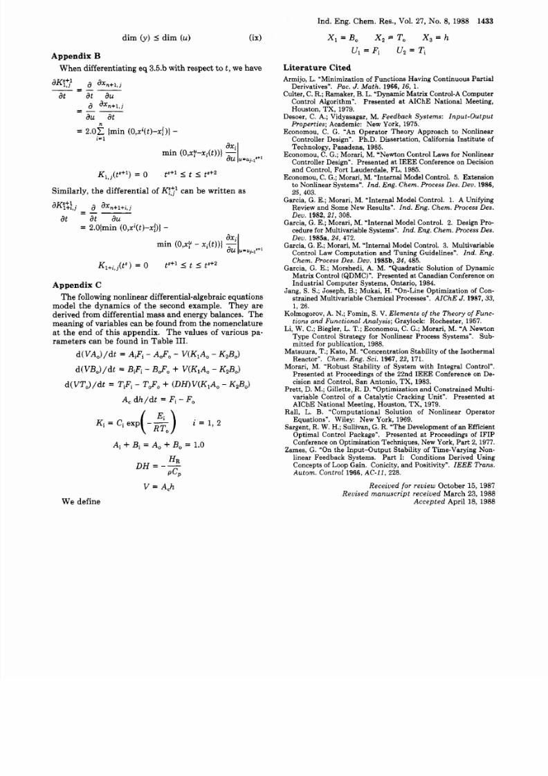
Appendix

B

When differentiating eq 3.5.b with respect to

t ,

we have

aK.,t,

a

axn+ l , j

a d X n + l , j

- = - -

at a t

au

au a t

= - -

n

i = l

= 2.0C

(min (~ , x ' ( t ) - x f ) j

Kl,j(t8+') = 0

ts+l

I I S + 2

Similarly, the differential of

Kj;

can be written as

W3,j

a a X n + l + i , j

= - -

at at a u

= 2.0{min ( O , x ( t ) - x f ) }

Appendix C

Th e following nonlinear differential-algebraic equations

model the dynamics of the second example. The y are

derived from differential mass and energy balances. Th e

meaning of variables can be found from th e nomenclature

at the end of this appendix. Th e values

of

various pa-

rameters can be found in Table

111.

d (VA,)/dt

= AiFi

A ,

- V(K1A0

KZB,)

d( VB,)/dt

= BiFi - B$, + V(KIAo

KZB,)

d(VT,) /d t

= TiFi 23,+ (DH)V(KIAo K&,)

A , d h / d t

= i - F,

Ai

+

Bi

=

A , + Bo

=

1.0

V =

A,h

We define

-

Dev. 1985a, 24 , 472.

Garcia. G. E.: Morari. M. Intern al Model Co ntrol. 3. Mu ltivariab le

Control Law Comp utation an d Tu ning Guidelines . Ind . Eng.

Chem . Process Des. Dev.

19858,

24 ,

485.

Garcia, G. E.; Morshed i, A. M. Quad ratic Solution of Dynam ic

Matrix Control (QDMC) . Presented a t Canadian Conference on

Industrial C omputer S ystems, Ontario, 1984.

Jang, S . S.; Joseph,

B.;

Mukai, H. On-Line Optimization of Con-

strained Multivariable Chemical Processes .

AI Ch E J.

1987,33,

1, 26.

Kolmogorov, A. N.; Fomin, S.V.Elem ents of t he Th eory of Func-

tions and Functional An alysis;

Graylock: Roc hester, 1957.

Li, W. C.; Biegler, L.

T.;

Econom ou, C. G.; Morari, M. A Newton

Typ e Control Strategy for Nonlinear Process Systems . Sub-

mitted for publication, 1988.

Matsuura, T.;Kato , M. Concentration Stability of the Isothermal

Reactor . Chem. Eng. Sci. 1967, 22 , 171.

Morari, M. Robust Sta bility of System with Integral Control .

Presented a t Proceedings of the 22nd IE EE Conference on De-

cision and Control, San Antonio, TX , 1983.

Pret t, D. M.; Gillette, R. D. Optimization a nd Constrained M ulti-

variable Control of a Catalytic Cracking Unit . Prese nted at

AIChE National Meeting, Houston, TX, 1979.

Rall,

L. B.

Com putatio nal Solution of Nonlinear Ope rator

Equ ations . Wiley: New York, 1969.

Sargent, R. W. H.; Sullivan, G. R. The Dev elopment of an Efficient

Optimal Control Package . Prese nted at Proceedings of IFIP

Conference on Optimization Techniqu es, New York, P ar t 2,1977.

Zames, G. On the Inpu t-Outp ut Stability of Time-Varying Non-

linear Feedback Systems. Pa rt I: Conditions Derived Using

Concepts of Loop Gain. Conicity, and Positivity . I EEE T r a n s.

Autom. Control

1966,

AC-1 I

228.

Rece ived f or rev iew October 15, 1987

Revised m anu scr ip t received Marc h 23, 1988

Ac c e p te d April 18, 1988

Documents

CSTR Reference Paper