CSE 613: Parallel Programming - Stony Brook Universityrezaul/Spring-2015/CSE613/CSE613-lecture-1.pdf“We used to joke that “parallel computing is the future, and always will be,”

“We used to joke that

“parallel computing is the future, and always will be,”

but the pessimists have been proven wrong.”

— Tony Hey

CSE 613: Parallel Programming

Department of Computer Science

SUNY Stony Brook

Spring 2015

Course Information

― Lecture Time: TuTh 2:30 pm - 3:50 pm

― Location: CS 2129, West Campus

― Instructor: Rezaul A. Chowdhury

― Office Hours: TuTh 12:00 pm - 1:30 pm, 1421 Computer Science

― Email: [email protected]

― TA: Unlikely

― Class Webpage:

http://www3.cs.stonybrook.edu/~rezaul/CSE613-S15.html

Prerequisites

― Required: Background in algorithms analysis

( e.g., CSE 373 or CSE 548 )

― Required: Background in programming languages ( C / C++ )

― Helpful but Not Required: Background in computer architecture

― Please Note: This is not a course on

― Programming languages

― Computer architecture

― Main Emphasis: Parallel algorithms

Topics to be Covered

The following topics will be covered

― Analytical modeling of parallel programs

― Scheduling

― Programming using the message-passing paradigm

and for shared address-space platforms

― Parallel algorithms for dense matrix operations,

sorting, searching, graphs, computational

geometry, and dynamic programming

― Concurrent data structures

― Transactional memory, etc.

Grading Policy

― Homeworks ( three: lowest score 5%, highest score 15%, and the

remaining one 10% ): 30%

― Group project ( one ): 55%

― Proposal: Feb 17

― Progress report: Mar 31

― Final demo / report: May 7

― Scribe note ( one lecture ): 10%

― Class participation & attendance: 5%

Programming Environment

This course is supported by an educational grant from

― Extreme Science and Engineering Discovery Environment ( XSEDE ):

https://www.xsede.org

We have access to the following two supercomputers

― Stampede ( Texas Advanced Comp. Center ): 6,400 nodes;

16 cores ( 2 Intel Sandy Bridge ) and 1/2 Intel Xeon Phi coprocessor(s) per node

― Trestles ( San Diego Supercomputer Center ): 300+ nodes;

32 cores ( 4 AMD Magny Cours processors ) per node

Programming Environment

World’s Most Powerful Supercomputers in November, 2014( www.top500.org )

Recommended Textbooks

― A. Grama, G. Karypis, V. Kumar, and A. Gupta. Introduction to Parallel

Computing (2nd Edition), Addison Wesley, 2003.

― J. JáJá. An Introduction to Parallel Algorithms (1st Edition), Addison

Wesley, 1992.

― T. Cormen, C. Leiserson, R. Rivest, and C. Stein. Introduction to Algorithms

(3rd Edition), MIT Press, 2009.

― M. Herlihy and N. Shavit. The Art of Multiprocessor Programming (1st

Edition), Morgan Kaufmann, 2008.

― P. Pacheco. Parallel Programming with MPI (1st Edition), Morgan

Kaufmann, 1996.

Why Parallelism?

Moore’s Law

Source: Wikipedia

Unicore Performance

Source: Jeff Preshing, 2012, http://preshing.com/20120208/a-look-back-at-single-threaded-cpu-performance/

Unicore Performance Has Hit a Wall!

Some Reasons

― Lack of additional ILP

( Instruction Level Hidden Parallelism )

― High power density

― Manufacturing issues

― Physical limits

― Memory speed

Unicore Performance: No Additional ILP

Exhausted all ideas to exploit hidden parallelism?

― Multiple simultaneous instructions

― Instruction Pipelining

― Out-of-order instructions

― Speculative execution

― Branch prediction

― Register renaming, etc.

“Everything that can be invented has been invented.”

— Charles H. Duell

Commissioner, U.S. patent office, 1899

Unicore Performance: High Power Density― Dynamic power, Pd ∝ V 2 f C

― V = supply voltage

― f = clock frequency

― C = capacitance

― But V ∝ f

― Thus Pd ∝ f 3

Source: Patrick Gelsinger, Intel Developer Forum, Spring 2004 ( Simon Floyd )

Unicore Performance: Manufacturing Issues

― Frequency, f ∝ 1 / s

― s = feature size ( transistor dimension )

― Transistors / unit area ∝ 1 / s2

― Typically, die size ∝ 1 / s

― So, what happens if feature size goes down by a factor of x?

― Raw computing power goes up by a factor of x4 !

― Typically most programs run faster by a factor of x3

without any change!

Source: Kathy Yelick and Jim Demmel, UC Berkeley

Unicore Performance: Manufacturing Issues

― Manufacturing cost goes up as feature size decreases― Cost of a semiconductor fabrication plant doubles

every 4 years ( Rock’s Law )

― CMOS feature size is limited to 5 nm ( at least 10 atoms )


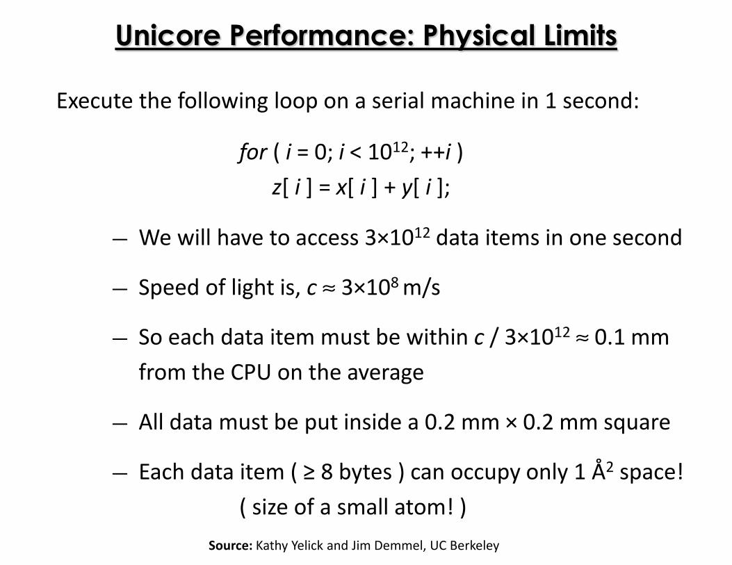
Unicore Performance: Physical Limits

Execute the following loop on a serial machine in 1 second:

for ( i = 0; i < 1012; ++i )

z[ i ] = x[ i ] + y[ i ];

― We will have to access 3×1012 data items in one second

― Speed of light is, c ≈ 3×108 m/s

― So each data item must be within c / 3×1012≈ 0.1 mm

from the CPU on the average

― All data must be put inside a 0.2 mm × 0.2 mm square

― Each data item ( ≥ 8 bytes ) can occupy only 1 Å2 space!

( size of a small atom! )


Unicore Performance: Memory Wall

Source: Rick Hetherington, Chief Technology Officer, Microelectronics, Sun Microsystems

Unicore Performance Has Hit a Wall!

Some Reasons

― Lack of additional ILP

( Instruction Level Hidden Parallelism )

― High power density

― Manufacturing issues

― Physical limits

― Memory speed

“Oh Sinnerman, where you gonna run to?”

— Sinnerman ( recorded by Nina Simone )

Where You Gonna Run To?

― Changing f by 20% changes performance by 13%

― So what happens if we overclock by 20%?

Source: Andrew A. Chien, Vice President of Research, Intel Corporation



― And underclock by 20%?





― And underclock by 20%?



Moore’s Law Reinterpreted

Source: Report of the 2011 Workshop on Exascale Programming Challenges

Cores / Processor ( General Purpose )


No Free Lunch for Traditional Software

Source: Simon Floyd, Workstation Performance: Tomorrow's Possibilities (Viewpoint Column)

Source: www.top500.org

Top 500 Supercomputing Sites ( Cores / Socket )

Insatiable Demand for Performance

Source: Patrick Gelsinger, Intel Developer Forum, 2008

Numerical Weather Prediction

Problem: ( temperature, pressure, …, humidity, wind velocity )

← f( longitude, latitude, height, time )

Approach ( very coarse resolution ):

― Consider only modeling fluid flow in the atmosphere

― Divide the entire global atmosphere into cubic cells of

size 1 mile × 1 mile × 1 mile each to a height of 10 miles

≈ 2 × 109 cells

― Simulate 7 days in 1 minute intervals

≈ 104 time-steps to simulate

― 200 floating point operations ( flop ) / cell / time-step

≈ 4 × 1015 floating point operations in total

― To predict in 1 hour ≈ 1 Tflop/s ( Tera flop / sec )

Some Useful Classifications

of Parallel Computers

Parallel Computer Memory Architecture( Distributed Memory )

― Each processor has its own

local memory ― no global

address space

― Changes in local memory by

one processor have no effect

on memory of other processors

― Communication network to connect inter-processor memory

― Programming ― Message Passing Interface ( MPI )

― Many once available: PVM, Chameleon, MPL, NX, etc.

Source: Blaise Barney, LLNL


Advantages

― Easily scalable

― No cache-coherency

needed among processors

― Cost-effective

Disadvantages

― Communication is user responsibility

― Non-uniform memory access

― May be difficult to map shared-memory data structures

to this type of memory organization


Parallel Computer Memory Architecture( Shared Memory )

― All processors access all memory

as global address space

― Changes in memory by one

processor are visible to all others

― Two types

― Uniform Memory Access

( UMA )

― Non-Uniform Memory Access

( NUMA )

― Programming ― Open Multi-Processing ( OpenMP )

― Cilk/Cilk++ and Intel Cilk Plus

― Intel Thread Building Block ( TBB ), etc.

UMA

NUMA



Advantages

― Easily scalable

― No cache-coherency

needed among processors

― Cost-effective

Disadvantages

― Communication is user responsibility

― Non-uniform memory access

― May be difficult to map shared-memory data structures

to this type of memory organization


Parallel Computer Memory Architecture( Hybrid Distributed-Shared Memory )

― The share-memory component

can be a cache-coherent SMP or

a Graphics Processing Unit (GPU)

― The distributed-memory

component is the networking of

multiple SMP/GPU machines

― Most common architecture

for the largest and fastest

computers in the world today

― Programming ― OpenMP / Cilk + CUDA / OpenCL + MPI, etc.


Flynn’s Taxonomy of Parallel Computers

Single Data

( SD )

Multiple Data

( MD )

Single Instruction

( SI )SISD SIMD

Multiple Instruction

( MI )MISD MIMD

Flynn’s classical taxonomy ( 1966 ):

Classification of multi-processor computer architectures along

two independent dimensions of instruction and data.


SISD

― A serial ( non-parallel ) computer

― The oldest and the most common

type of computers

― Example: Uniprocessor unicore

machinesSource: Blaise Barney, LLNL


SIMD

― A type of parallel computer

― All PU’s run the same instruction at any given clock cycle

― Each PU can act on a different data item

― Synchronous ( lockstep ) execution

― Two types: processor arrays and vector pipelines

― Example: GPUs ( Graphics Processing Units )



MISD


― Very few ever existed

MIMD


― Synchronous /asynchronous

execution

― Examples: most modern

supercomputers, parallel

computing clusters,

multicore PCsSource: Blaise Barney, LLNL

Parallel Algorithms

Warm-up

“The way the processor industry is going, is to add more and more cores, but

nobody knows how to program those things. I mean, two, yeah; four, not

really; eight, forget it.”

— Steve Jobs, NY Times interview, June 10 2008

Parallel Algorithms Warm-up (1)

Consider the following loop:

for i = 1 to n do

C[ i ] ← A[ i ] × B[ i ]

― Suppose you have an infinite number of processors/cores

― Ignore all overheads due to scheduling, memory accesses,

communication, etc.

― Suppose each operation takes a constant amount of time

― How long will this loop take to complete execution?


Consider the following loop:

for i = 1 to n do

C[ i ] ← A[ i ] × B[ i ]

― Suppose you have an infinite number of processors/cores

― Ignore all overheads due to scheduling, memory accesses,

communication, etc.

― Suppose each operation takes a constant amount of time


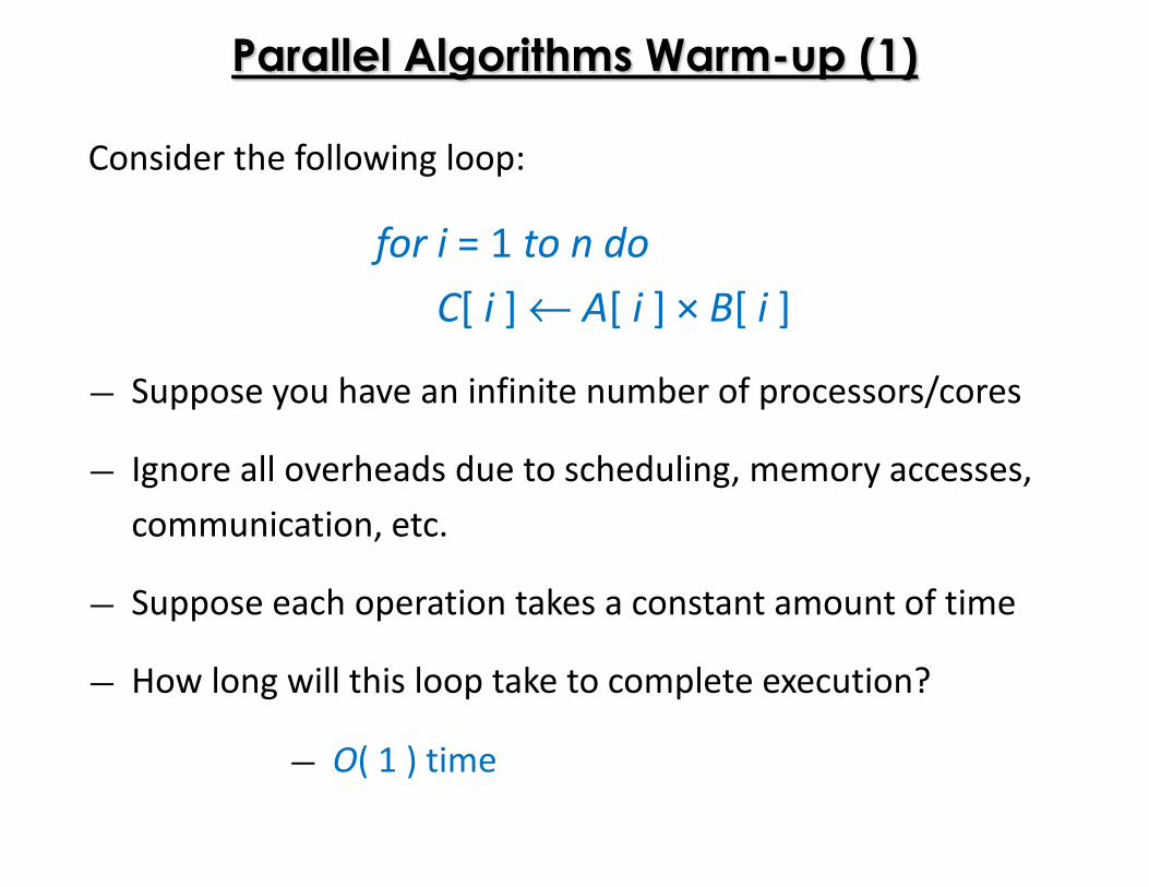
― O( 1 ) time


Now consider the following loop:

c ← 0

for i = 1 to n do

c ← c + A[ i ] × B[ i ]



Now consider the following loop:

c ← 0

for i = 1 to n do

c ← c + A[ i ] × B[ i ]


― O( log n ) time


Now consider quicksort:

QSort( A )

if |A|≤ 1 return A

else p ← A[ rand( |A| ) ]

return QSort( { x ∈ A: x < p } )

# { p } #

QSort( { x ∈ A: x > p } )

― Assuming that A is split in the middle everytime, and the two

recursive calls can be made in parallel, how long will this

algorithm take?


Now consider quicksort:

QSort( A )

if |A|≤ 1 return A

else p ← A[ rand( |A| ) ]

return QSort( { x ∈ A: x < p } )

# { p } #

QSort( { x ∈ A: x > p } )

― Assuming that A is split in the middle everytime, and the two

recursive calls can be made in parallel, how long will this

algorithm take?

― O( log2 n ) ( if partitioning takes logarithmic time )

― O( log n ) ( but can be partitioned in constant time )

Documents

CSE 613: Parallel Programming - Stony Brook Universityrezaul/Spring-2015/CSE613/CSE613-lecture-1.pdf“We used to joke that “parallel computing is the future, and always will be,”