CSE 5526: Boltzmann Machines - mr-pc.org

1 CSE 5526: Boltzmann Machines

CSE 5526: Introduction to Neural Networks

Boltzmann Machines


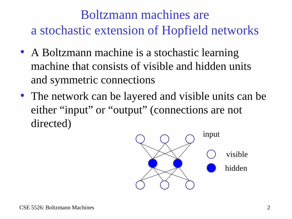
Boltzmann machines are a stochastic extension of Hopfield networks

• A Boltzmann machine is a stochastic learning machine that consists of visible and hidden units and symmetric connections

• The network can be layered and visible units can be either “input” or “output” (connections are not directed)

input

hidden

visible


In general, the network is fully connected


Boltzmann machines have the same energy function as Hopfield networks

• Because of symmetric connections, the energy function of neuron configuration 𝐱𝐱 is:

𝐸𝐸 𝐱𝐱 = −12��𝑤𝑤𝑗𝑗𝑗𝑗𝑥𝑥𝑗𝑗𝑥𝑥𝑗𝑗

𝑗𝑗𝑗𝑗

= 𝐱𝐱𝑇𝑇𝑊𝑊𝐱𝐱

• Can we start there and derive a probability

distribution over configurations?


The Boltzmann-Gibbs distribution defines probabilities from energies

• Consider a physical system with many states. • Let 𝑝𝑝𝑗𝑗 denote the probability of occurrence of state 𝑖𝑖 • Let 𝐸𝐸𝑗𝑗 denote the energy of state 𝑖𝑖

• From statistical mechanics, when the system is in thermal equilibrium, it satisfies

𝑝𝑝𝑗𝑗 =1𝑍𝑍

exp −𝐸𝐸𝑗𝑗𝑇𝑇

where 𝑍𝑍 = � exp −𝐸𝐸𝑗𝑗𝑇𝑇

𝑗𝑗

• Z is called the partition function, and 𝑇𝑇 is called the temperature

• The Boltzmann-Gibbs distribution


Remarks

• Lower energy states have higher probability of occurrences

• As 𝑇𝑇 decreases, the probability is concentrated on a small subset of low energy states


Boltzmann-Gibbs distribution example

• Consider 𝑬𝑬 = [1, 2, 3] • At 𝑇𝑇 = 10,

• 𝒑𝒑� = exp −𝑬𝑬𝑇𝑇

= 0.905, 0.819, 0.741

• 𝑍𝑍 = ∑ 𝑝𝑝�𝑗𝑗𝑗𝑗 = 0.905 + 0.819 + 0.741 = 2.464

• 𝒑𝒑 = 1𝑍𝑍𝒑𝒑� = [0.367, 0.332, 0.301]



• Consider 𝑬𝑬 = [1, 2, 3] • At 𝑇𝑇 = 1,


= 0.368, 0.135, 0.050

• 𝑍𝑍 = ∑ 𝑝𝑝�𝑗𝑗𝑗𝑗 = 0.368 + 0.135 + 0.050 = 0.553

• 𝒑𝒑 = 1𝑍𝑍𝒑𝒑� = [0.665, 0.245, 0.090]



• Consider 𝑬𝑬 = [1, 2, 3] • At 𝑇𝑇 = 0.1,


= 4.54 ⋅ 10−5, 2.06 ⋅ 10−9, 9.36 ⋅ 10−14

• 𝑍𝑍 = ∑ 𝑝𝑝�𝑗𝑗𝑗𝑗 = 4.54 ⋅ 10−5 + 2.06 ⋅ 10−9 + 9.36 ⋅ 10−14 = 4.54 ⋅ 10−5

• 𝒑𝒑 = 1𝑍𝑍𝒑𝒑� = [0.99995, 4.54 ⋅ 10−5, 2.06 ⋅ 10−9]


Boltzmann-Gibbs distribution applied to Hopfield network energy function

𝑝𝑝 𝐱𝐱 =1𝑍𝑍

exp −1𝑇𝑇𝐸𝐸 𝐱𝐱 =

1𝑍𝑍

exp1

2𝑇𝑇𝐱𝐱𝑇𝑇𝑊𝑊𝐱𝐱

• Partition function For 𝑁𝑁 neurons, involves 2𝑁𝑁 terms

𝑍𝑍 = �𝑝𝑝 𝐱𝐱𝐱𝐱

• Marginal over 𝐻𝐻 of the neurons Involves 2𝐻𝐻 terms

𝑝𝑝 𝐱𝐱𝛼𝛼 = �𝑝𝑝 𝐱𝐱𝛼𝛼 , 𝐱𝐱𝛽𝛽𝐱𝐱𝛽𝛽


Boltzmann machines are unsupervised probability models

• The primary goal of Boltzmann machine learning is to produce a network that models the probability distribution of observed data (at visible neurons) • Such a net can be used for pattern completion, as a part of

an associative memory, etc. • What do we want to do with it?

• Compute the probability of a new observation • Learn parameters of the model from data • Estimate likely values completing partial observations


Compute the probability of a new observation

• Divide the entire net into the subset 𝐱𝐱𝛼𝛼 of visible units and 𝐱𝐱𝛽𝛽 of hidden units

• Given parameters 𝑊𝑊, compute likelihood of observation 𝐱𝐱𝛼𝛼

𝑝𝑝 𝐱𝐱𝛼𝛼 = �𝑝𝑝(𝐱𝐱)𝐱𝐱𝛽𝛽

= �1𝑍𝑍

exp −1𝑇𝑇𝐸𝐸 𝐱𝐱

𝐱𝐱𝛽𝛽

= �1𝑍𝑍

exp1

2𝑇𝑇𝐱𝐱𝑇𝑇𝑊𝑊𝐱𝐱

𝐱𝐱𝛽𝛽


Learning can be performed by gradient descent

• The objective of Boltzmann machine learning is to maximize the likelihood of the visible units taking on training patterns by adjusting W

• Assuming that each pattern of the training sample is statistically independent, the log probability of the training sample is:

𝐿𝐿 𝐰𝐰 = log�𝑃𝑃(𝐱𝐱𝛼𝛼)𝐱𝐱𝛼𝛼

= � log 𝑃𝑃(𝐱𝐱𝛼𝛼)𝐱𝐱𝛼𝛼


Log likelihood of data has two terms

𝐿𝐿 𝐰𝐰 = log�𝑃𝑃(𝐱𝐱𝛼𝛼)𝐱𝐱𝛼𝛼

= � log 𝑃𝑃(𝐱𝐱𝛼𝛼)𝐱𝐱𝛼𝛼

= � log�1𝑍𝑍

exp −𝐸𝐸 𝐱𝐱𝑇𝑇

𝐱𝐱𝛽𝛽𝐱𝐱𝛼𝛼

= � log� exp −𝐸𝐸 𝐱𝐱𝑇𝑇

𝐱𝐱𝛽𝛽

− log 𝑍𝑍𝐱𝐱𝛼𝛼

= � log� exp −𝐸𝐸 𝐱𝐱𝑇𝑇

𝐱𝐱𝛽𝛽

− log� exp −𝐸𝐸 𝐱𝐱𝑇𝑇

𝐱𝐱𝐱𝐱𝛼𝛼


Gradient of log likelihood of data

𝜕𝜕𝜕𝜕(𝐰𝐰)𝜕𝜕𝑤𝑤𝑗𝑗𝑗𝑗

= �𝜕𝜕

𝜕𝜕𝑤𝑤𝑗𝑗𝑗𝑗log� exp −

𝐸𝐸 𝐱𝐱𝑇𝑇

𝐱𝐱𝛽𝛽

−𝜕𝜕

𝜕𝜕𝑤𝑤𝑗𝑗𝑗𝑗log� exp −

𝐸𝐸 𝐱𝐱𝑇𝑇

𝐱𝐱𝐱𝐱𝛼𝛼

= �− 1𝑇𝑇∑ exp −𝐸𝐸 𝐱𝐱

𝑇𝑇𝜕𝜕𝐸𝐸 𝐱𝐱𝜕𝜕𝑤𝑤𝑗𝑗𝑗𝑗𝐱𝐱𝛽𝛽

∑ exp −𝐸𝐸 𝐱𝐱𝑇𝑇𝐱𝐱𝛽𝛽

+

1𝑇𝑇∑ exp −𝐸𝐸 𝐱𝐱

𝑇𝑇𝜕𝜕𝐸𝐸 𝐱𝐱𝜕𝜕𝑤𝑤𝑗𝑗𝑗𝑗𝐱𝐱

∑ exp −𝐸𝐸 𝐱𝐱𝑇𝑇𝐱𝐱𝐱𝐱𝛼𝛼



• Then, since 𝜕𝜕𝜕𝜕(𝐱𝐱)𝜕𝜕𝑤𝑤𝑗𝑗𝑗𝑗

= −𝑥𝑥𝑗𝑗𝑥𝑥𝑗𝑗

𝜕𝜕𝐿𝐿(𝐰𝐰)𝜕𝜕𝑤𝑤𝑗𝑗𝑗𝑗

=1𝑇𝑇� �

exp −𝐸𝐸 𝐱𝐱𝑇𝑇 𝑥𝑥𝑗𝑗𝑥𝑥𝑗𝑗

∑ exp −𝐸𝐸 𝐱𝐱𝑇𝑇𝐱𝐱𝛽𝛽𝐱𝐱𝛽𝛽

−∑ exp −𝐸𝐸 𝐱𝐱

𝑇𝑇 𝑥𝑥𝑗𝑗𝑥𝑥𝑗𝑗𝐱𝐱

𝑍𝑍𝐱𝐱𝛼𝛼

=1𝑇𝑇

��𝑃𝑃 𝐱𝐱𝛽𝛽 𝐱𝐱𝛼𝛼 𝑥𝑥𝑗𝑗𝑥𝑥𝑗𝑗𝐱𝐱𝛽𝛽𝐱𝐱𝛼𝛼

−��𝑃𝑃(𝐱𝐱)𝑥𝑥𝑗𝑗𝑥𝑥𝑗𝑗𝐱𝐱𝐱𝐱𝛼𝛼

training patterns constant w.r.t. ∑ ∙𝐱𝐱𝛼𝛼



𝜕𝜕𝐿𝐿(𝐰𝐰)𝜕𝜕𝑤𝑤𝑗𝑗𝑗𝑗

=1𝑇𝑇𝜌𝜌𝑗𝑗𝑗𝑗+ − 𝜌𝜌𝑗𝑗𝑗𝑗−

• Where 𝜌𝜌𝑗𝑗𝑗𝑗+ = ∑ ∑ 𝑃𝑃 𝐱𝐱𝛽𝛽 𝐱𝐱𝛼𝛼 𝑥𝑥𝑗𝑗𝑥𝑥𝑗𝑗𝐱𝐱𝛽𝛽𝐱𝐱𝛼𝛼 = ∑ 𝐸𝐸𝐱𝐱𝛽𝛽|𝐱𝐱𝛼𝛼{𝑥𝑥𝑗𝑗𝑥𝑥𝑗𝑗}𝐱𝐱𝛼𝛼 • is the mean correlation between neurons i and j when the

visible units are “clamped” to 𝐱𝐱𝛼𝛼

• And 𝜌𝜌𝑗𝑗𝑗𝑗− = 𝐾𝐾∑ 𝑃𝑃 𝐱𝐱 𝑥𝑥𝑗𝑗𝑥𝑥𝑗𝑗𝐱𝐱 = 𝐸𝐸𝐱𝐱{𝑥𝑥𝑗𝑗𝑥𝑥𝑗𝑗} • is the mean correlation between i and j when the machine

operates without “clamping”


Maximization of 𝐿𝐿 𝐰𝐰

• To maximize 𝐿𝐿 𝐰𝐰 , we use gradient ascent:

△ 𝑤𝑤𝑗𝑗𝑗𝑗 = 𝜀𝜀𝜕𝜕𝐿𝐿 𝐰𝐰𝜕𝜕𝑤𝑤𝑗𝑗𝑗𝑗

=𝜀𝜀𝑇𝑇𝜌𝜌𝑗𝑗𝑗𝑗+ − 𝜌𝜌𝑗𝑗𝑗𝑗−

= 𝜂𝜂 𝜌𝜌𝑗𝑗𝑗𝑗+ − 𝜌𝜌𝑗𝑗𝑗𝑗− where the learning rate 𝜂𝜂 incorporates the temperature 𝑇𝑇


Positive and negative phases

• Thus there are two phases to the learning process: 1. Positive phase: the net operates in the “clamped”

condition, where visible units take on training patterns with the desired probability distribution

2. Negative phase: the net operates freely without the influence of external input


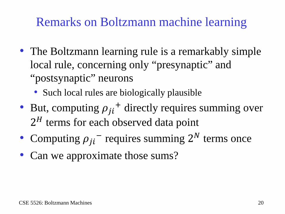
Remarks on Boltzmann machine learning

• The Boltzmann learning rule is a remarkably simple local rule, concerning only “presynaptic” and “postsynaptic” neurons • Such local rules are biologically plausible

• But, computing 𝜌𝜌𝑗𝑗𝑗𝑗+ directly requires summing over 2𝐻𝐻 terms for each observed data point

• Computing 𝜌𝜌𝑗𝑗𝑗𝑗− requires summing 2𝑁𝑁 terms once • Can we approximate those sums?


Sampling methods can approximate expectations (difficult integrals/sums)

• Want to compute 𝜌𝜌𝑗𝑗𝑗𝑗− = ∑ 𝑃𝑃 𝐱𝐱 𝑥𝑥𝑗𝑗𝑥𝑥𝑗𝑗𝐱𝐱 = 𝐸𝐸𝐱𝐱 𝑥𝑥𝑗𝑗𝑥𝑥𝑗𝑗 • We can approximate that expectation as

𝜌𝜌𝑗𝑗𝑗𝑗− = 𝐸𝐸𝐱𝐱 𝑥𝑥𝑗𝑗𝑥𝑥𝑗𝑗 ≈1𝑁𝑁�𝑥𝑥𝑗𝑗𝑥𝑥𝑗𝑗𝐱𝐱𝑛𝑛

• Where 𝐱𝐱𝑛𝑛 are samples drawn from 𝑃𝑃 𝐱𝐱𝑛𝑛

• In general 𝐸𝐸𝐱𝐱 𝑓𝑓(𝐱𝐱) ≈ 1𝑁𝑁∑ 𝑓𝑓 𝐱𝐱𝑛𝑛𝐱𝐱𝑛𝑛

• The sum converges to the true expectation as the number of samples goes to infinity

• This is called Monte Carlo integration / summation


Gibbs sampling can draw samples from intractable distributions

• Many high-dimensional probability distributions are difficult to compute or sample from

• But Gibbs sampling can draw samples from them • If you can compute the probability of some variables

given others • This is typically the case in graphical models, including

Boltzmann machines • This kind of approach is called Markov chain

Monte Carlo (MCMC)


Gibbs sampling can draw samples from intractable distributions

• Consider a K-dimensional random vector 𝐱𝐱 = (𝑥𝑥1, … , 𝑥𝑥𝐾𝐾)𝑇𝑇

• Suppose we know the conditional distributions 𝑝𝑝 𝑥𝑥𝑘𝑘 𝑥𝑥1, … , 𝑥𝑥𝑘𝑘−1, 𝑥𝑥𝑘𝑘+1, … , 𝑥𝑥𝐾𝐾 = 𝑝𝑝 𝑥𝑥𝑘𝑘 𝐱𝐱∼𝑘𝑘

• Then by sampling each 𝑥𝑥𝑘𝑘 in turn (or randomly), the distribution of samples will eventually converge to

𝑝𝑝 𝐱𝐱 = 𝑝𝑝(𝑥𝑥1, … , 𝑥𝑥𝐾𝐾) • Note: it can be difficult to know how long to sample


Gibbs sampling algorithm

• For iteration n: 𝑥𝑥1(𝑛𝑛) is drawn from 𝑝𝑝 𝑥𝑥1 𝑥𝑥2, … , 𝑥𝑥𝐾𝐾 … 𝑥𝑥𝑘𝑘(𝑛𝑛) is drawn from 𝑝𝑝 𝑥𝑥𝑘𝑘 𝑥𝑥1, … , 𝑥𝑥𝑘𝑘−1, 𝑥𝑥𝑘𝑘+1, … , 𝑥𝑥𝐾𝐾 … 𝑥𝑥𝐾𝐾(𝑛𝑛) is drawn from 𝑝𝑝 𝑥𝑥𝐾𝐾 𝑥𝑥1, … , 𝑥𝑥𝐾𝐾−1

• Each iteration samples each random variable once in the natural order

• Newly sampled values are used immediately (i.e., asynchronous sampling)


Gibbs sampling in Boltzmann machines

• Need 𝑝𝑝 𝑥𝑥𝑘𝑘 𝑥𝑥1, … , 𝑥𝑥𝑘𝑘−1, 𝑥𝑥𝑘𝑘+1, … , 𝑥𝑥𝐾𝐾 = 𝑝𝑝 𝑥𝑥𝑘𝑘 𝐱𝐱∼𝑘𝑘 • Can compute from Boltzmann-Gibbs distribution

𝑝𝑝 𝑥𝑥𝑘𝑘 𝐱𝐱∼𝑘𝑘 =𝑝𝑝 𝑥𝑥𝑘𝑘 = 1, 𝐱𝐱∼𝑘𝑘

𝑝𝑝 𝑥𝑥𝑘𝑘 = 1, 𝐱𝐱∼𝑘𝑘 + 𝑝𝑝 𝑥𝑥𝑘𝑘 = −1, 𝐱𝐱∼𝑘𝑘

=

1𝑍𝑍 exp −𝐸𝐸

+

𝑇𝑇1𝑍𝑍 exp −𝐸𝐸

+

𝑇𝑇 + 1𝑍𝑍 exp −𝐸𝐸

−

𝑇𝑇

=1

1 + exp 1𝑇𝑇 𝐸𝐸+ − 𝐸𝐸−

= 𝜎𝜎Δ𝐸𝐸𝑇𝑇


So Boltzmann machines use stochastic neurons with sigmoid activation

• Neuron 𝑘𝑘 is connected to all other neurons:

𝑣𝑣𝑘𝑘 = �𝑤𝑤𝑘𝑘𝑗𝑗𝑥𝑥𝑗𝑗𝑗𝑗

• It is then updated stochastically so that

𝑥𝑥𝑘𝑘 = � 1 with prob. 𝜑𝜑 𝑣𝑣𝑘𝑘 −1 with prob. 1 − 𝜑𝜑(𝑣𝑣𝑘𝑘)

• Where

𝜑𝜑 𝑣𝑣 =1

1 + exp −𝑣𝑣𝑇𝑇


Prob. of flipping a single neuron

• Consider the prob. of flipping a single neuron k:

𝑃𝑃 𝑥𝑥𝑘𝑘 → −𝑥𝑥𝑘𝑘 =1

1 + exp ∆𝐸𝐸𝑘𝑘2𝑇𝑇

where ∆𝐸𝐸𝑗𝑗 is the energy change due to the flip (proof is a homework problem)

• So a change that decreases the energy is more likely than that increasing the energy


Simulated annealing

• As the temperature T decreases • The average energy of a stochastic system decreases • It reaches the global minimum as 𝑇𝑇 → 0 • So for optimization problems, should favor low temps

• But, convergence is slow at low temps • due to trapping at local minima

• Simulated annealing is a stochastic optimization technique that gradually decreases 𝑇𝑇 • To get the best of both worlds


Simulated annealing (cont.)

• No guarantee for the global minimum, but higher chances for lower local minima

• Boltzmann machines use simulated annealing to gradually lower T


Full Boltzmann machine training algorithm

• The entire algorithm consists of the following nested loops: 1. Loop over all training data points, accumulating

gradient of each weight 2. For each data point, compute expectation 𝑥𝑥𝑗𝑗𝑥𝑥𝑗𝑗 with 𝐱𝐱𝛼𝛼

clamped and free 3. Compute expectations using simulated annealing,

gradually decreasing T 4. For each T, sample the state of the entire net a number

of times using Gibbs sampling


Remarks on Boltzmann machine training

• Boltzmann machines are extremely slow to train • but work well once they are trained

• Because of its computational complexity, the algorithm has only been applied to toy problems

• But: the restricted Boltzmann machine is much easier to train, stay tuned…


An example

• The encoder problem (see blackboard)

• Ackley, Hinton, Sejnowski (1985)

Documents

CSE 5526: Boltzmann Machines - mr-pc.org