CSE 454 Infrmation Retrieval & Indexing. Information Extraction INet Advertising Security Cloud Computing UI & Revisiting Class Overview Network Layer

CSE 454

Infrmation Retrieval & Indexing

Information Extraction

INet Advertising

Security

Cloud Computing

UI & Revisiting

Class Overview

Network Layer

Crawling

IR - Ranking

Indexing

Query processing

Other Cool Stuff

Content Analysis

A Closeup View

10/19 – IR & Indexing

10/21 – Google & Alta Vista

10/26 – Pagerank

Standard Web Search Engine Architecture

crawl theweb

create an inverted

index

store documents,check for duplicates,

extract links

inverted index

DocIds

Slide adapted from Marti Hearst / UC Berkeley]

Search engine servers

userquery

show results To user

Relevance

• Complex concept that has been studied for some time– Many factors to consider – People often disagree when making relevance

judgments

• Retrieval models make various assumptions about relevance to simplify problem– e.g., topical vs. user relevance– e.g., binary vs. multi-valued relevance

from Croft, Metzler, Strohman. © Addison Wesley

Retrieval Model Overview

• Older models– Boolean retrieval– Overlap Measures– Vector Space model

• Probabilistic Models– BM25– Language models

• Combining evidence– Inference networks– Learning to Rank


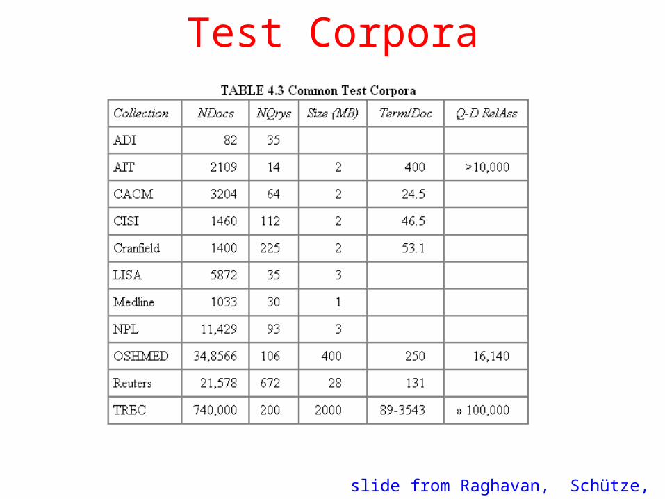
Test Corpora

slide from Raghavan, Schütze, Larson

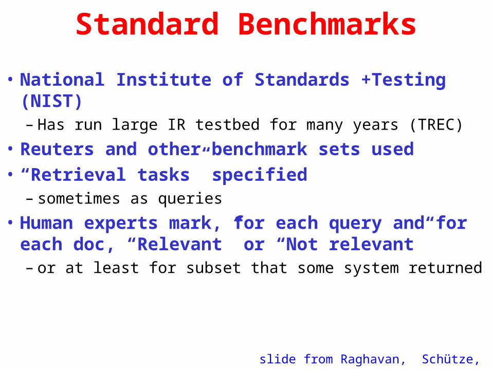
Standard Benchmarks

• National Institute of Standards +Testing (NIST)– Has run large IR testbed for many years (TREC)

• Reuters and other benchmark sets used• “Retrieval tasks” specified

– sometimes as queries

• Human experts mark, for each query and for each doc, “Relevant” or “Not relevant”– or at least for subset that some system returned


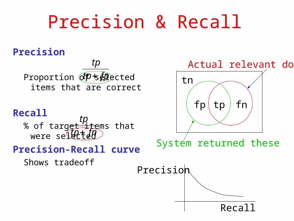
Precision & Recall

Precision

Proportion of selected items that are correct

Recall% of target items that were

selected

Precision-Recall curveShows tradeoff

tn

fp tp fn

System returned these

Actual relevant docsfptp

tp

fntp

tp

Recall

Precision

Precision/Recall• Can get high recall (but low precision)

– Retrieve all docs on all queries!

• Recall is a non-decreasing function of the number of docs retrieved– Precision usually decreases (in a good system)

• Difficulties in using precision/recall – Binary relevance– Should average over large corpus/query ensembles– Need human relevance judgements– Heavily skewed by corpus/authorship


Precision-Recall Curves• May return any # of results ordered by similarity

• By varying numbers of docs (levels of recall)– Produce a precision-recall curve


Q1

Q2

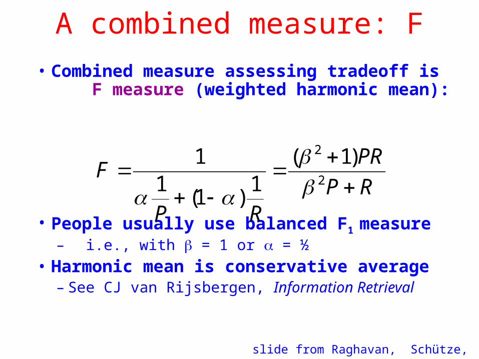
A combined measure: F

• Combined measure assessing tradeoff is F measure (weighted harmonic mean):

• People usually use balanced F1 measure– i.e., with = 1 or = ½

• Harmonic mean is conservative average– See CJ van Rijsbergen, Information Retrieval

RP

PR

RP

F

2

2 )1(1

)1(1

1


Boolean Retrieval

• Two possible outcomes for query processing– TRUE and FALSE– “exact-match” retrieval– simplest form of ranking

• Query specified w/ Boolean operators– AND, OR, NOT– proximity operators also used


Query

• Which plays of Shakespeare contain the words Brutus AND Caesar but NOT Calpurnia?


Term-document incidence

1 if play contains word, 0 otherwise

Tempest Hamlet Othello MacbethAntony 0 0 0 1Brutus 0 1 0 0Caesar 0 1 1 1

Calpurnia 0 0 0 0Cleopatra 0 0 0 0

mercy 1 1 1 1worser 1 1 1 0


Booleans over Incidence Vectors

• So we have a 0/1 vector for each term.

• To answer query: take the vectors for Brutus, Caesar and Calpurnia (complemented) bitwise AND.

• 110100 AND 110111 AND 101111 = 100100.


Boolean Retrieval• Advantages

– Results are predictable, relatively easy to explain– Many different features can be incorporated– Efficient processing since many documents can be

eliminated from search• Disadvantages

– Effectiveness depends entirely on user– Simple queries usually don’t work well– Complex queries are difficult


Interlude• Better Models Coming Soon:

– Vector Space model– Probabilistic Models

• BM25• Language models

• Shared Issues – What to Index– Punctuation– Case Folding– Stemming– Stop Words– Spelling– Numbers

Issues in what to index

• Cooper’s vs. Cooper vs. Coopers.• Full-text vs. full text vs. {full, text} vs. fulltext.• résumé vs. resume.

Cooper’s concordance of Wordsworth was published in 1911. The applications of full-text retrieval are legion: they include résumé scanning, litigation support and searching published journals on-line.


Punctuation• Ne’er: use language-specific, handcrafted

“locale” to normalize.

• State-of-the-art: break up hyphenated sequence.

• U.S.A. vs. USA - use locale.

• a.out


Numbers• 3/12/91

• Mar. 12, 1991

• 55 B.C.

• B-52

• 100.2.86.144– Generally, don’t index as text– Creation dates for docs


Case folding• Reduce all letters to lower case

• Exception: upper case in mid-sentence– e.g., General Motors– Fed vs. fed– SAIL vs. sail


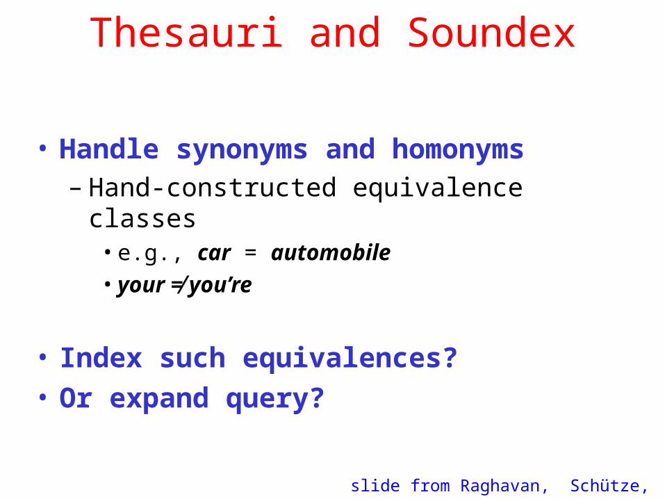
Thesauri and Soundex

• Handle synonyms and homonyms– Hand-constructed equivalence classes

• e.g., car = automobile

• your ≠ you’re

• Index such equivalences?

• Or expand query?


Spell Correction• Look for all words within (say) edit distance 3

(Insert/Delete/Replace) at query time– e.g., Alanis Morisette

• Spell correction is expensive and slows the query (up to a factor of 100)– Invoke only when index returns zero matches?– What if docs contain mis-spellings?


Lemmatization• Reduce inflectional/variant forms to base form

– am, are, is be

– car, cars, car's, cars' car

the boy's cars are different colors

the boy car be different color


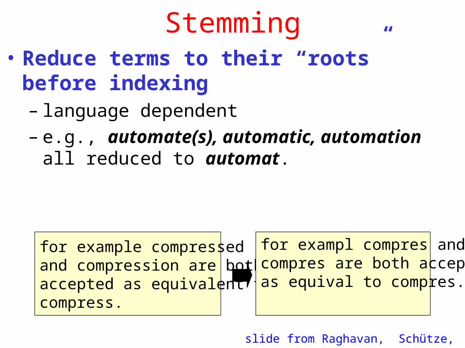
Stemming• Reduce terms to their “roots” before indexing

– language dependent– e.g., automate(s), automatic, automation all reduced to

automat.

for example compressed and compression are both accepted as equivalent to compress.

for exampl compres andcompres are both acceptas equival to compres.


Porter’s algorithm

• Common algorithm for stemming English

• Conventions + 5 phases of reductions– phases applied sequentially– each phase consists of a set of commands– sample convention: Of the rules in a compound

command, select the one that applies to the longest suffix.

• Porter’s stemmer available: http//www.sims.berkeley.edu/~hearst/irbook/porter.html


Typical rules in Porter

• sses ss

• ies i

• ational ate

• tional tion


Challenges

• Sandy

• Sanded

• Sander

Sand ???


Beyond Term Search• Phrases?

• Proximity: Find Gates NEAR Microsoft.– Index must capture position info in docs.

• Zones in documents: Find documents with (author = Ullman) AND (text contains automata).


Ranking search results• Boolean queries give inclusion or exclusion of docs.

• Need to measure proximity from query to each doc.

• Whether docs presented to user are singletons, or a group of docs covering various aspects of the query.


Ranking models in IR• Key idea:

– We wish to return in order the documents most likely to be useful to the searcher

• To do this, we want to know which documents best satisfy a query– An obvious idea is that if a document talks about a topic more then it is a

better match

• A query should then just specify terms that are relevant to the information need, without requiring that all of them must be present– Document relevant if it has a lot of the terms


Retrieval Model Overview

• Older models– Boolean retrieval– Overlap Measures– Vector Space model

• Probabilistic Models– BM25– Language models

• Combining evidence– Inference networks– Learning to Rank


Binary term presence matrices• Record whether a document contains a word:

document is binary vector in {0,1}v

• Idea: Query satisfaction = overlap measure:

Antony and Cleopatra Julius Caesar The Tempest Hamlet Othello Macbeth

Antony 1 1 0 0 0 1

Brutus 1 1 0 1 0 0

Caesar 1 1 0 1 1 1

Calpurnia 0 1 0 0 0 0

Cleopatra 1 0 0 0 0 0

mercy 1 0 1 1 1 1

worser 1 0 1 1 1 0

YX


Overlap matching

• What are the problems with the overlap measure?

• It doesn’t consider:– Term frequency in document– Term scarcity in collection

• (How many documents mention term?)

– Length of documents


Many Overlap Measures

|)||,min(|

||

||||

||

||||

||||

||2

||

21

21

DQ

DQ

DQ

DQ

DQDQ

DQ

DQ

DQ

Simple matching (coordination level match)

Dice’s Coefficient

Jaccard’s Coefficient

Cosine Coefficient

Overlap Coefficient


Documents as vectors• Each doc j can be viewed as a vector of tf values, one

component for each term

• So we have a vector space– terms are axes

– docs live in this space

– even with stemming, may have 20,000+ dimensions

• (The corpus of documents gives us a matrix, which we could also view as a vector space in which words live – transposable data)


Vector Space Representation

Documents that are close to query (measured using vector-space metric) => returned first.

Query


TF x IDF

)/log(* kikik nNtfw

C in T term of frequency document inverse idf

D document in T term of frequencytf

D document in k termT

kk

ikik

ik

nNidf

kk log

kk T contain that C indocuments of number then

C collection the indocuments of number total N


BM25 Popular and effective ranking algorithm based on

binary independence model– adds document and query term weights

– N = number of doc, ni = num containing term I– R, ri = encode relevance info (if avail, otherwise = 0)– fi = freq of term I in doc; qfi = freq in doc– k1, k2 and K are parameters, values set empirically

• k1 weights tf component as fi increases• k2 = weights query term weight• K normalizes

adapted from Croft, Metzler, Strohman. © Addison Wesley

43

Simple Formulas

But How Process Efficiently?

Copyright © Weld 2002-2007

44

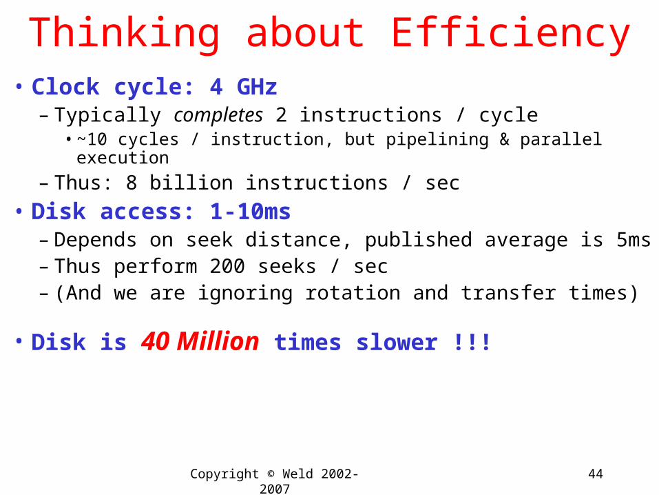
Thinking about Efficiency• Clock cycle: 4 GHz

– Typically completes 2 instructions / cycle• ~10 cycles / instruction, but pipelining & parallel execution

– Thus: 8 billion instructions / sec

• Disk access: 1-10ms– Depends on seek distance, published average is 5ms– Thus perform 200 seeks / sec– (And we are ignoring rotation and transfer times)

• Disk is 40 Million times slower !!!


45

Retrieval

Document-term matrix

t1 t2 . . . tj . . . tm nf

d1 w11 w12 . . . w1j . . . w1m 1/|d1| d2 w21 w22 . . . w2j . . . w2m 1/|d2|

. . . . . . . . . . . . . .

di wi1 wi2 . . . wij . . . wim 1/|di|

. . . . . . . . . . . . . . dn wn1 wn2 . . . wnj . . . wnm 1/|dn|

wij is the weight of term tj in document di

Most wij’s will be zero.Copyright © Weld 2002-2007

46

Naïve Retrieval

Consider query Q = (q1, q2, …, qj, …, qn), nf = 1/|q|.

How evaluate Q?

(i.e., compute the similarity between q and every document)?

Method 1: Compare Q with every doc.

Document data structure:

di : ((t1, wi1), (t2, wi2), . . ., (tj, wij), . . ., (tm, wim ), 1/|di|)

– Only terms with positive weights are kept.

– Terms are in alphabetic order.

Query data structure: Q : ((t1, q1), (t2, q2), . . ., (tj, qj), . . ., (tm, qm ), 1/|q|)


48

Observation

• Method 1 is not efficient– Needs to access most non-zero entries in doc-term matrix.

• Solution: Use Index (Inverted File)– Data structure to permit fast searching.

• Like an Index in the back of a text book.– Key words --- page numbers.– E.g, “Etzioni, 40, 55, 60-63, 89, 220”– Lexicon– Occurrences


49

Search Processing (Overview)1. Lexicon search

– E.g. looking in index to find entry

2. Retrieval of occurrences– Seeing where term occurs

3. Manipulation of occurrences– Going to the right page


50

Simple Index for One Document

A file is a list of words by positionFirst entry is the word in position 1 (first word)Entry 4562 is the word in position 4562 (4562nd word)Last entry is the last wordAn inverted file is a list of positions by word!

POS1

10

20

30

36

FILE

a (1, 4, 40)entry (11, 20, 31)file (2, 38)list (5, 41)position (9, 16, 26)positions (44)word (14, 19, 24, 29, 35, 45)words (7)4562 (21, 27)

INVERTED FILE

aka “Index”


Requirements for Search• Need index structure

– Must handle multiple documents– Must support phrase queries– Must encode TF/IDF values– Must minimize disk seeks & reads

Copyright © Weld 2002-2007 51

a (1, 4, 40)entry (11, 20, 31)file (2, 38)list (5, 41)position (9, 16, 26)positions (44)

t1 t2 … tm

d1 w11 w12 … w1m

d2 w21 w22 … w2m

…dn wn1 wn2 …wnm




+

How Store Index?

Oracle Database?

Unix File System?

aaaaddand…

…docID # pos1, … …

Lexicon Occurrence List

The Solution • Inverted Files for Multiple Documents

– Broken into Two Files • Lexicon

– Hashtable on disk (one read)– Nowadays: stored in main memory

• Occurrence List– Stored on Disk – “Google Filesystem”

Copyright © Weld 2002-2007 54

aaaaddand…

…docID # pos1, … …

Lexicon Occurrence List

55

Inverted Files for Multiple Documents

107 4 322 354 381 405232 6 15 195 248 1897 1951 2192677 1 481713 3 42 312 802

WORD NDOCS PTR

jezebel 20

jezer 3

jezerit 1

jeziah 1

jeziel 1

jezliah 1

jezoar 1

jezrahliah 1

jezreel 39jezoar

34 6 1 118 2087 3922 3981 500244 3 215 2291 301056 4 5 22 134 992

DOCID OCCUR POS 1 POS 2 . . .

566 3 203 245 287

67 1 132. . .

“jezebel” occurs6 times in document 34,3 times in document 44,4 times in document 56 . . .

LEXICON

OCCURENCE INDEX

• One method. Alta Vista uses alternative

…


56

Many Variations Possible

• Address space (flat, hierarchical)

• Record term-position information

• Precalculate TF-IDF info

• Stored header, font & tag info

• Compression strategies


Other Features Stored in Index• Page Rank• Query word in color on page?• # images on page• # outlinks on page• URL length• Page edit recency

• Page Classifiers (20+)– Spam– Adult– Actor – Celebrity – Athlete– Product / review– Tech company– Church– Homepage– ….

Amit Singhai says Google uses over 200 such features [NY Times 2008-06-03]

58

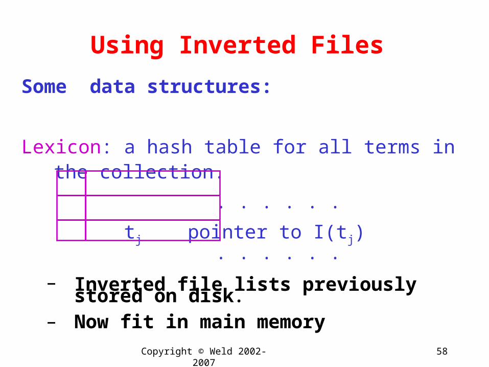
Using Inverted Files

Some data structures:

Lexicon: a hash table for all terms in the collection.

. . . . . .

tj pointer to I(tj) . . . . . .

– Inverted file lists previously stored on disk.

– Now fit in main memory


59

The Lexicon

• Grows Slowly (Heap’s law)– O(n) where n=text size; is constant ~0.4 – 0.6– E.g. for 1GB corpus, lexicon = 5Mb– Can reduce with stemming (Porter algorithm)

• Store lexicon in file in lexicographic order– Each entry points to loc in occurrence file

(aka inverted file list)


60

Using Inverted Files

Several data structures:

2. For each term tj, create a list (occurrence file list) that

contains all document ids that have tj.

I(tj) = { (d1, w1j),

(d2, …

… }

– di is the document id number of the ith document.

– Weights come from freq of term in doc

– Only entries with non-zero weights are kept.


61

More Elaborate Inverted File

Several data structures:

2. For each term tj, create a list (occurrence file list) that

contains all document ids that have tj.

I(tj) = { (d1, freq, pos1, … posk),

(d2, …

… }

– di is the document id number of the ith document.

– Weights come from freq of term in doc

– Only entries with non-zero weights are kept.


62

Inverted files continued

More data structures:

3. Normalization factors of documents are pre-computed and stored similarly to lexicon

nf[i] stores 1/|di|.


63

Retrieval Using Inverted Files

initialize all sim(q, di) = 0

for each term tj in q

find I(t) using the hash table

for each (di, wij) in I(t)

sim(q, di) += qj wij

for each (relevant) document di

sim(q, di) = sim(q, di) nf[i]

sort documents in descending similarities and display the top k to the user;


64

Observations about Method 2• If doc d doesn’t contain any term of query q,

then d won’t be considered when evaluating q.

• Only non-zero entries in the columns of the document-term matrix which correspond to query terms … are used to evaluate the query.

• Computes the similarities of multiple documents simultaneously (w.r.t. each query word)


67

Efficiency versus Flexibility

• Storing computed document weights is good for efficiency, but bad for flexibility.

– Recomputation needed if TF and IDF formulas change and/or TF and DF information changes.

• Flexibility improved by storing raw TF, DF information, but efficiency suffers.

• A compromise– Store pre-computed TF weights of documents.– Use IDF weights with query term TF weights

instead of document term TF weights.Copyright © Weld 2002-2007

68

How Inverted Files are Created

Crawler Repository Scan ForwardIndex

Sort

SortedIndex

Scan

NF(docs)

Lexicon

InvertedFileList

ptrsto

docs


69

Creating Inverted Files Crawler Repository Scan ForwardIndex

Sort

SortedIndex

Scan

NF(docs)

Lexicon

InvertedFileList

Repository• File containing all documents downloaded• Each doc has unique ID• Ptr file maps from IDs to start of doc in repository

ptrsto

docs


70


Sort

SortedIndex

Scan

NF(docs)

Lexicon

InvertedFileList

ptrsto

docs

NF ~ Length of each document

Term Doc #I 1did 1enact 1julius 1caesar 1I 1was 1killed 1i' 1the 1capitol 1brutus 1killed 1me 1so 2let 2it 2be 2with 2caesar 2the 2noble 2brutus 2hath 2told 2you 2

caesar 2was 2ambitious 2

Forward Index Pos1234567


71


Sort

SortedIndex

Scan

NF(docs)

Lexicon

InvertedFileList

ptrsto

docs

Term Doc #ambitious 2be 2brutus 1brutus 2capitol 1caesar 1caesar 2caesar 2did 1enact 1hath 1I 1I 1i' 1it 2julius 1killed 1killed 1let 2me 1noble 2so 2the 1the 2told 2you 2was 1was 2with 2

Term Doc #I 1did 1enact 1julius 1caesar 1I 1was 1killed 1i' 1the 1capitol 1brutus 1killed 1me 1so 2let 2it 2be 2with 2caesar 2the 2noble 2brutus 2hath 2told 2you 2caesar 2was 2ambitious 2

Sorted Index

(positional info as well)


72


Sort

SortedIndex

Scan

NF(docs)

Lexicon

InvertedFileList

WORD NDOCS PTR

jezebel 20

jezer 3

jezerit 1

jeziah 1

jeziel 1

jezliah 1

jezoar 1

jezrahliah 1

jezreel 39jezoar

34 6 1 118 2087 3922 3981 500244 3 215 2291 301056 4 5 22 134 992

DOCID OCCUR POS 1 POS 2 . . .

566 3 203 245 287

67 1 132. . .

ptrsto

docs

Lexicon

Inverted File List


75

Stop lists• Language-based stop list:

– words that bear little meaning– 20-500 words– http://www.dcs.gla.ac.uk/idom/ir_resources/linguistic_utils/stop_words

• Subject-dependent stop lists• Removing stop words

– From document– From query

From Peter Brusilovsky Univ Pittsburg INFSCI 2140


76

Stemming• Are there different index terms?

– retrieve, retrieving, retrieval, retrieved, retrieves…

• Stemming algorithm: – (retrieve, retrieving, retrieval, retrieved, retrieves)

retriev– Strips prefixes of suffixes (-s, -ed, -ly, -ness)– Morphological stemming


77

Stemming Continued • Can reduce vocabulary by ~ 1/3• C, Java, Perl versions, python, c#

www.tartarus.org/~martin/PorterStemmer

• Criterion for removing a suffix – Does "a document is about w1" mean the same as – a "a document about w2"

• Problems: sand / sander & wand / wander

• Commercial SEs use giant in-memory tables


78

Compression• What Should We Compress?

– Repository– Lexicon– Inv Index

• What properties do we want?– Compression ratio– Compression speed– Decompression speed– Memory requirements– Pattern matching on compressed text– Random access


79

Inverted File Compression

Each inverted list has the form 1 2 3 ; , , , ... ,

tt ff d d d d

A naïve representation results in a storage overhead of ( ) * logf n N

This can also be stored as 1 2 1 1; , ,...,t tt f ff d d d d d

Each difference is called a d-gap. Since

( ) ,d gaps N each pointer requires fewer than

Trick is encoding …. since worst case ….

log N bits.

Assume d-gap representation for the rest of the talk, unless stated otherwise

Slides adapted from Tapas Kanungo and David Mount, Univ Maryland


80

Text CompressionTwo classes of text compression methods• Symbolwise (or statistical) methods

– Estimate probabilities of symbols - modeling step– Code one symbol at a time - coding step– Use shorter code for the most likely symbol– Usually based on either arithmetic or Huffman coding

• Dictionary methods– Replace fragments of text with a single code word – Typically an index to an entry in the dictionary.

• eg: Ziv-Lempel coding: replaces strings of characters with a pointer to a previous occurrence of the string.

– No probability estimates needed

Symbolwise methods are more suited for coding d-gaps


81

Classifying d-gap Compression Methods:

• Global: each list compressed using same model– non-parameterized: probability distribution for d-gap sizes is

predetermined.

– parameterized: probability distribution is adjusted according to certain parameters of the collection.

• Local: model is adjusted according to some parameter, like the frequency of the term

• By definition, local methods are parameterized.


82

Conclusion• Local methods best

• Parameterized global models ~ non-parameterized– Pointers not scattered randomly in file

• In practice, best index compression algorithm is:

– Local Bernoulli method (using Golomb coding)• Compressed inverted indices usually faster+smaller than

– Signature files– Bitmaps

Local < Parameterized Global < Non-parameterized Global

Not by much
