Embed Size (px)
Citation preview

CSE 255
ASSIGNMENT 1 WINTER 2015
ALOK SINGH A53035244
1. Identify a dataset to study
1a) Identify Data Source: The dataset that I chose to perform this analysis is from Beeradvocate. The data was available at http://snap.stanford.edu/data/Beeradvocate.txt.gz. This dataset is in following format:
● beer/name : Name of the beer ● beer/beerId : Unique beer identification ● beer/brewerId : Unique ID identifying the brewer ● beer/style : Category that the beer falls into ● beer/ABV : Alcohol by volume ● review/profileName: Reviewer’s profile name / user ID ● review/time : UNIX time when review was written ● review/aroma : Rating based on how the beer smells [15] ● review/palate : Rating based on how the beer interacts with the palate [15] ● review/taste : Rating based on how the beer actually tastes [15] ● review/appearance: Rating based on how the beer looks [15] ● review/text : Personal observations made by the review in text format ● review/overall : Cumulative experience of the beer is encapsulated in this rating [15]
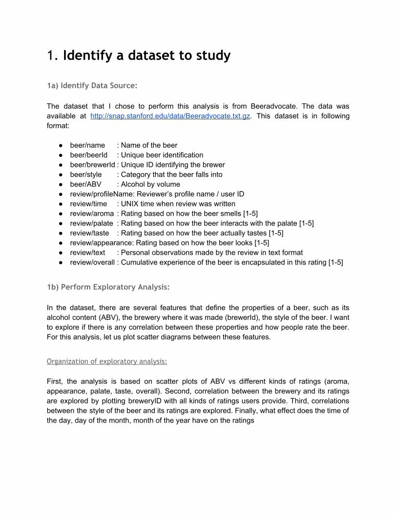
1b) Perform Exploratory Analysis: In the dataset, there are several features that define the properties of a beer, such as its alcohol content (ABV), the brewery where it was made (brewerId), the style of the beer. I want to explore if there is any correlation between these properties and how people rate the beer. For this analysis, let us plot scatter diagrams between these features.
Organization of exploratory analysis: First, the analysis is based on scatter plots of ABV vs different kinds of ratings (aroma, appearance, palate, taste, overall). Second, correlation between the brewery and its ratings are explored by plotting breweryID with all kinds of ratings users provide. Third, correlations between the style of the beer and its ratings are explored. Finally, what effect does the time of the day, day of the month, month of the year have on the ratings
Beers with >5% ABV tend to get higher Aroma ratings, with all of them getting >3 star rating
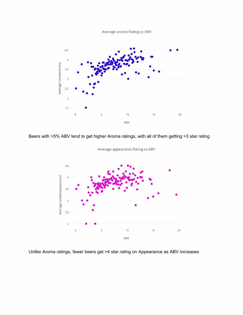
Unlike Aroma ratings, fewer beers get >4 star rating on Appearance as ABV increases

Beers with low ABV content tend to low palate rating
Taste ratings follow similar pattern as the palate ratings, as expected
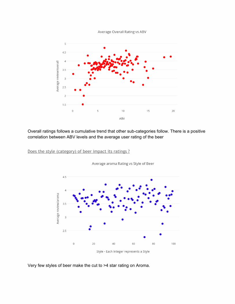
Overall ratings follows a cumulative trend that other subcategories follow. There is a positive correlation between ABV levels and the average user rating of the beer
Does the style (category) of beer impact its ratings ?
Very few styles of beer make the cut to >4 star rating on Aroma.
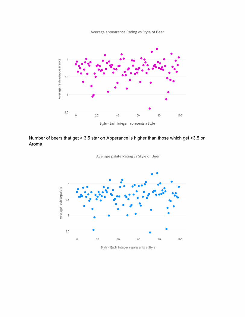
Number of beers that get > 3.5 star on Apperance is higher than those which get >3.5 on Aroma
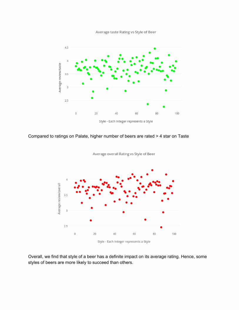
Compared to ratings on Palate, higher number of beers are rated > 4 star on Taste
Overall, we find that style of a beer has a definite impact on its average rating. Hence, some styles of beers are more likely to succeed than others.
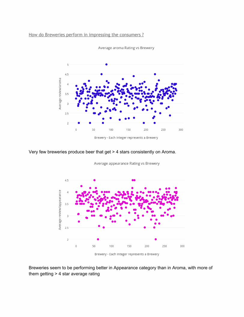
How do Breweries perform in impressing the consumers ?
Very few breweries produce beer that get > 4 stars consistently on Aroma.
Breweries seem to be performing better in Appearance category than in Aroma, with more of them getting > 4 star average rating
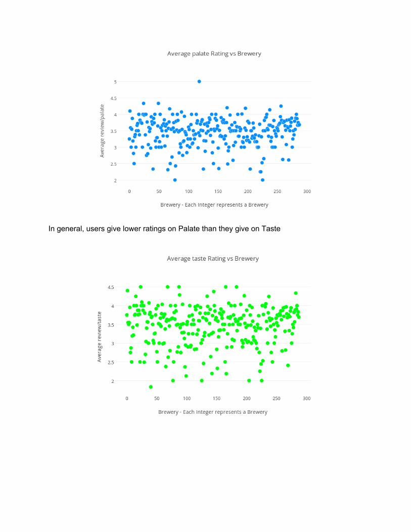
In general, users give lower ratings on Palate than they give on Taste
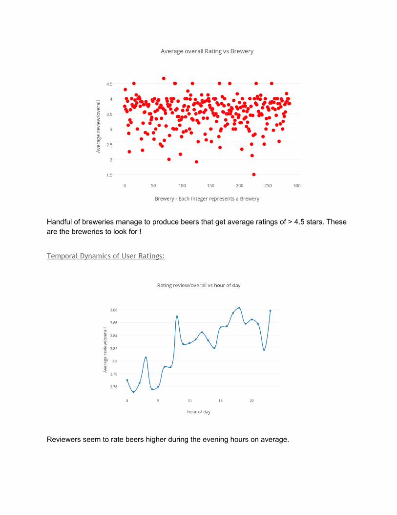
Handful of breweries manage to produce beers that get average ratings of > 4.5 stars. These are the breweries to look for !
Temporal Dynamics of User Ratings:
Reviewers seem to rate beers higher during the evening hours on average.
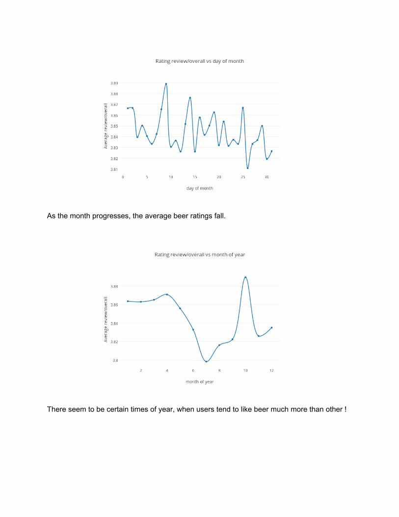
As the month progresses, the average beer ratings fall.
There seem to be certain times of year, when users tend to like beer much more than other !
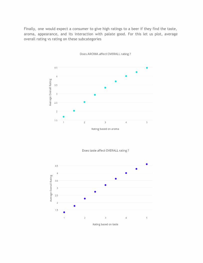
Finally, one would expect a consumer to give high ratings to a beer if they find the taste, aroma, appearance, and its interaction with palate good. For this let us plot, average overall rating vs rating on these subcategories
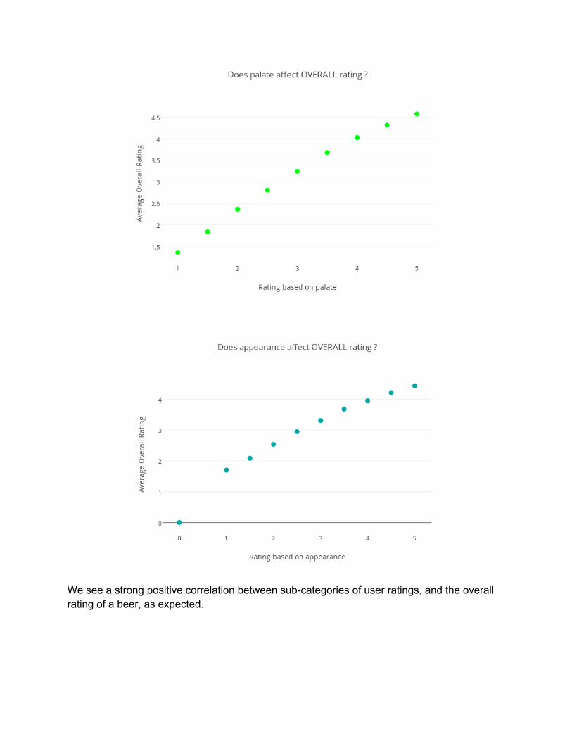
We see a strong positive correlation between subcategories of user ratings, and the overall rating of a beer, as expected.
2. Identify a predictive task: For this assignment, it is best to take the perspective of a ‘brewery’. Let us assume that a brewery is planning to launch a new beer into market. This brewery would like to understand how this beer will be received by its consumers. It makes business sense to predict reviewers’ rating, based on features of a beer. This will help the brewery expand its offering in most profitable way. Since, a consumer bases his/her decision to consume a beer based on their ‘overall’ experience of the beer, we will use ‘overall’ rating as our main objective function. From the exploratory analysis, it has been observed that ‘overall’ rating has a strong positive correlation with how a beer tastes, smells, appears, interacts with palate. Hence, our model’s success is measured by how accurately it predicts ‘overall’ rating of a beer. With this objective of launching highly rated beer, we want to train a model on past data and use it to predict success of new beers. We will use first 60,000 reviews for training, and next 60,000 review for testing. Our evaluation will be based on “Mean Square Error” of results predicted by the model, when compared with existing reviews. We will use linear regression as baseline predictor, and will search for a model that does substantially better than the linear model in predicting overall rating of a beer.
3. Literature Review: The dataset that I chose to perform this analysis is from Beeradvocate [5]. Other similar datasets include reviews from website Ratebeer [6] and CellarTracker [7]. Beeradvocate [5] provides online user reviews about beer based on explicit categories or aspects of the product. This provides a rich set of heterogeneous data, where textual information and these explicit ratings can be used to build language models, as described in [1]. The Pale Lager Model described in [1] models aspects and their ratings as a function of words that used describe in textual data. Once a language model is built through supervised learning on this training data, it can be used to summarize reviews and extrapolate missing ratings [1]. In contrast with using multiple ratings along with text data to form predictive models, there exists techniques that use single rating value in combination with textual information, to generate prodcut recommendation models [8], discover features [9] and perform sentiment analysis [10]. There are works that either use only explicit user ratings in numeric form, such as Matrix factorization [11] or others which just use textual data from reviews, such as clustering and
topic modeling [12, 13]. Beeradvocate data [5] contains timestamps of each user review. This provides a potential opportunity to student the temporal dynamics of user ratings on a given product, and on other reviews. [2] describes a latent factor model that takes into account the temporal aspects of review data to predict how user preferences might change over time. It aims to model personal development of users as they gain expertise on the subject at hand. [2] attempts to capture the difference between a novice and an expert. Models that account for temporal dynamics have proved to give much better prediction performance [8, 14]. Influence of current ratings on the behaviour of new users has been studied in [15], and authors in [16] study community dynamics by investigating how new users respond when existing ratings affect their view. [3] demonstrates the use of statistical models which uncover hidden dimensions in rating data, and combines them with topics in review text. One key finding of [3] related to the beer database it used is that beer style has an impact on its user rating. Other work that combines review text and rating is [17], which highlights how user’s ratings are impacted by the value they associate to each aspect of a product. Other works, such as [18, 19] also perform global feature discovery. Global features that are common to all products are referred to as aspects. Authors in [4] propose a method that uses conceptual probabilistic model to discover patterns of progression in a given time series event sequence, by grouping them based on their evolution behavior and segmenting them into several progression stages. [4] claims that each sequence of event contains several ‘stages’, where duration of each stage varies across sequences. It also aims to cluster sequence of events that follow common stage progression paths, using unsupervised learning techniques. With regards to Beeradvocate dataset [5], [4] provides insights into most frequent events at a given progression stage for two classes. Other works which find sequence of events that are common to other sequences through episode mining [20, 21]
4. Features: In this assignment, ‘overall’ rating is identified as the single most important value that we want to predict. There are several factors that could play a role in this ‘overall’ indicator that captures what a user experiences, and in most cases determines how economically successful a beer would be. List of factors that have potential impact on ‘overall’ rating of beer:
1. beer/style: as we have seen, certain styles of beer got higher ‘average’ overall rating. Hence, it is possible that the likelihood of some styles succeeding in having a positive impact on consumer experience are high. [taken: Yes]
2. beer/name: sometime, the name and packaging of a product can give an extra push to a quality product. Marketing personnel spend a lot of time in coming up with branding solutions that enhance a product exerpeince. In the context of current modelling, we want to ignore the effect of product packaging/naming on the overall rating. [taken: No]
3. beer/ABV: alcohol is an essential part of a beer, that separates it from nonalcoholic beverages. We have observed in the scatter plots, that beers which had >4 overall rating almost always had >5% ABV. Hence, we want to include ABV value as a valid feature in our model. [taken: Yes]
4. beer/brewerId: certain breweries are more likely to produce good bear products consistently, hence knowledge of brewery does play a role in predicting whether a beer will get good rating. Knowledge of brewery itself encapsulates information about underlying manufacturing process, the craftmanship, and other subtle factors that go into making a good beer. Hence, we will take brewery into account, as a feature. [taken: Yes]
5. review/time: we have seen in exploratory analysis that different time stamps do have an impact on the beer’s overall rating. However, the underlying context of this assignment, from a brewery’s perspective, is to make a rating prediction about beer’s overall success in the market, as compared to is seasonal success. For this reason, review/time is not taken as a feature in this analysis. [taken: No]
In the training set, there are 99 unique styles and 251 unique breweries in the 57809 reviews we are using for training our model. Each of these styles and breweries have different impact on the final rating of the product. Hence, each feature vector will have 99 columns for styles, 251 columns for breweries and 1 column for ABV value. In preprocessing, we will have to extract information about brewery, style, and ABV value of each review tuple, and construct a feature vector that contains this information in binary format. Our feature vector will be a numpy array of 57809 rows and 351 columns. Each tuple will have information about beer’s feature in this order: [ABV(1), style (99), brewerId (251)]
Preprocessing of data:
● Training dataset contains 57809 reviews. Originally I wanted to get the first 60,000 reviews from the Beeradvocate dataset, however 2191 reviews contained ‘empty’ beer/ABV values, hence I had to remove those reviews from the training set.
● Test dataset contains 4000 reviews that are selected from a set disjoint with the training set. Since the original Beeradvocate data contains much more beer/styles and beer/brewerIds than those present in the training set. Test set sampling was subject to
constraint that the beer/style and beer/brewerId of any review must be one of those found in the training set.
● Converted the Y_test and Y_train (rating) vector values to integer to be compatible with Scikit library.
5. Model: We want to choose a model that provides the right balance between Bias error and Variance error. In current assignment, we have used limited data set (<100K) to train the model. The prediction task involves prediction of a continuous target variable y, hence we want to select a valid Regression model (i.e. perform Supervised Learning). In current context, we will use Mean Squared Error as a measure of accuracy of the model. We want to use Regularized Regression models that prevent overfitting. Lasso and Ridge are two such models that fit this category. Lasso uses L1 norm for regularization. Lasso has the flexibility of making coefficients equal to zero, and therefore eliminating irrelevant input variables from contributing to the target variable. In comparison, Ridge uses L2 norm for regularization. Ridge regression cannot zero out coefficients. Elastic net model combines the strength of Ridge Regression and Lasso by linearly combining L1 and L2 penalties. Hence, we will compare Lasso and Ridge with Elastic net model results. If a set of input variables are highly correlated among themselves, LASSO tends to pick only one of them and reduces the other coefficients to zero. Lasso is not good for grouped selection. Since our feature vector contains fairly uncorrelated features (ABV, Style, Brewery), Lasso is well suited for the task. Another model that was considered for comparison is Decision Tree Regressor. It is a nonparametric supervised learning method that predicts target variable by learning simple decision rules inferred from the data features. As the depth of the tree is increased, the model captures finer details of the training dataset. Decision trees are prone to overfitting as small variations in training data might result in completely different decision tree. We will run this model for comparison with Lasso model. In addition to above models, for comparison purposes, some ensemble methods based on averaging and boosting are also evaluated. Ensemble methods combine the predictions of several base predictors, and hence present a possibility of improving basic linear model based predictions. However, cross validation has not been performed here to check for overfitting.
Parameter selection for Lasso Model: To select the best value of alpha, 6 evenly logspaced values were taken from 104 to 101. In the end, the alpha which produced maximum coefficient of determination R2 for the prediction was taken for Lasso model.
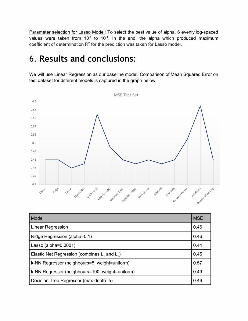
6. Results and conclusions: We will use Linear Regression as our baseline model. Comparison of Mean Squared Error on test dataset for different models is captured in the graph below:
Model MSE
Linear Regression 0.46
Ridge Regression (alpha=0.1) 0.46
Lasso (alpha=0.0001) 0.44
Elastic Net Regression (combines L1 and L2) 0.45
kNN Regressor (neighbours=5, weight=uniform) 0.57
kNN Regressor (neighbours=100, weight=uniform) 0.49
Decision Tree Regressor (maxdepth=5) 0.46
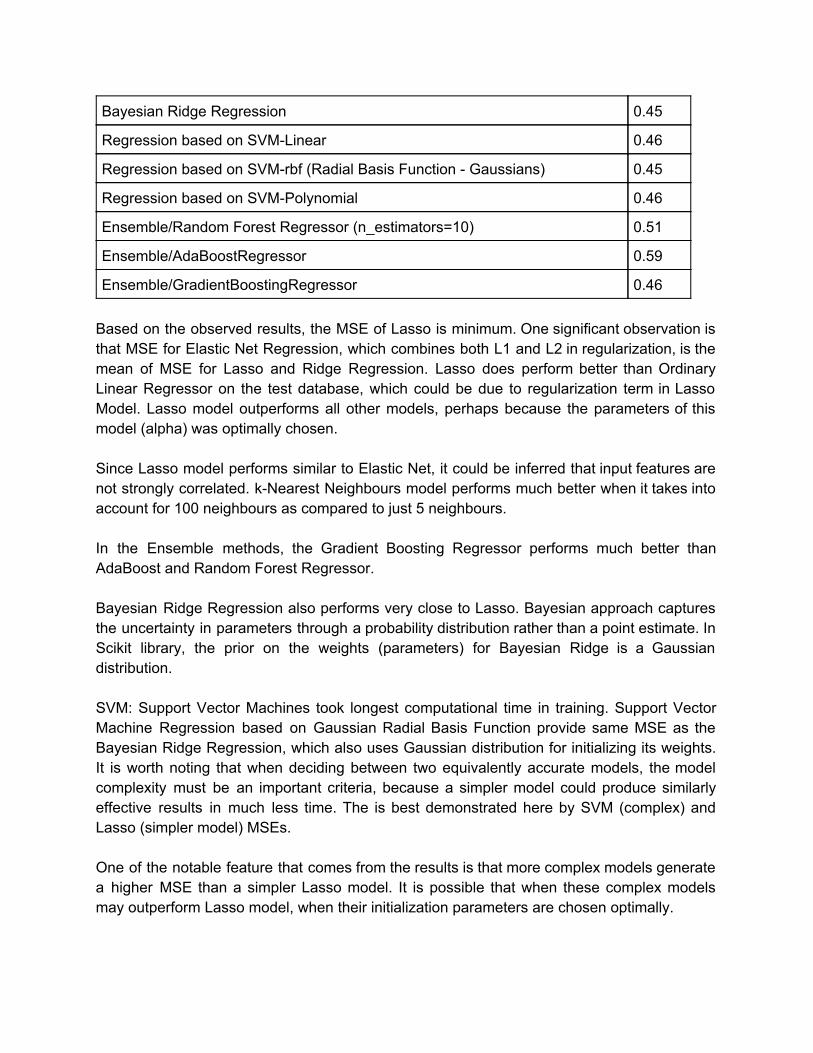
Bayesian Ridge Regression 0.45
Regression based on SVMLinear 0.46
Regression based on SVMrbf (Radial Basis Function Gaussians) 0.45
Regression based on SVMPolynomial 0.46
Ensemble/Random Forest Regressor (n_estimators=10) 0.51
Ensemble/AdaBoostRegressor 0.59
Ensemble/GradientBoostingRegressor 0.46 Based on the observed results, the MSE of Lasso is minimum. One significant observation is that MSE for Elastic Net Regression, which combines both L1 and L2 in regularization, is the mean of MSE for Lasso and Ridge Regression. Lasso does perform better than Ordinary Linear Regressor on the test database, which could be due to regularization term in Lasso Model. Lasso model outperforms all other models, perhaps because the parameters of this model (alpha) was optimally chosen. Since Lasso model performs similar to Elastic Net, it could be inferred that input features are not strongly correlated. kNearest Neighbours model performs much better when it takes into account for 100 neighbours as compared to just 5 neighbours. In the Ensemble methods, the Gradient Boosting Regressor performs much better than AdaBoost and Random Forest Regressor. Bayesian Ridge Regression also performs very close to Lasso. Bayesian approach captures the uncertainty in parameters through a probability distribution rather than a point estimate. In Scikit library, the prior on the weights (parameters) for Bayesian Ridge is a Gaussian distribution. SVM: Support Vector Machines took longest computational time in training. Support Vector Machine Regression based on Gaussian Radial Basis Function provide same MSE as the Bayesian Ridge Regression, which also uses Gaussian distribution for initializing its weights. It is worth noting that when deciding between two equivalently accurate models, the model complexity must be an important criteria, because a simpler model could produce similarly effective results in much less time. The is best demonstrated here by SVM (complex) and Lasso (simpler model) MSEs. One of the notable feature that comes from the results is that more complex models generate a higher MSE than a simpler Lasso model. It is possible that when these complex models may outperform Lasso model, when their initialization parameters are chosen optimally.
In conclusion, this exercise has demonstrated that choosing a model is a process, where several competing models must be optimized by picking the right parameters. Literature online points to guidelines for choosing best learning models for solving prediction problems. Eventually, the best model for a given dataset can only be found by training these models on the dataset, optimizing their parameters and selecting the best one.
[1] McAuley, J., J. Leskovec, and D. Jurafsky. “Learning Attitudes and Attributes from MultiAspect Reviews.” In 2012 IEEE 12th International Conference on Data Mining (ICDM), 1020–25, 2012. doi:10.1109/ICDM.2012.110. [2] McAuley, Julian, and Jure Leskovec. “From Amateurs to Connoisseurs: Modeling the Evolution of User Expertise through Online Reviews.” arXiv:1303.4402 [physics], March 18, 2013. http://arxiv.org/abs/1303.4402. [3] McAuley, J., & Leskovec, J. (2013). Hidden Factors and Hidden Topics: Understanding Rating Dimensions with Review Text. In Proceedings of the 7th ACM Conference on Recommender Systems (pp. 165–172). New York, NY, USA: ACM. doi:10.1145/2507157.2507163 [4] Yang, Jaewon, Julian McAuley, Jure Leskovec, Paea LePendu, and Nigam Shah. “Finding Progression Stages in TimeEvolving Event Sequences.” In Proceedings of the 23rd International Conference on World Wide Web, 783–94. WWW ’14. New York, NY, USA: ACM, 2014. doi:10.1145/2566486.2568044. [5] BeerAdvocate Dataset: http://snap.stanford.edu/data/Beeradvocate.txt.gz [6] Ratebeer Dataset: http://snap.stanford.edu/data/Ratebeer.txt.gz [7] Cellartracker Dataset: http://snap.stanford.edu/data/cellartracker.txt.gz. [8] J. Bennett and S. Lanning. The Netflix prize. In KDD Cup and Workshop, 2007 [9] A. Popescu and O. Etzioni. Extracting product features and opinions from reviews. In HLT, 2005. [10] P. Turney. Thumbs up or thumbs down? semantic orientation applied to unsupervised classification of reviews. In ACL, 2002. [11] Y. Koren, R. Bell, and C. Volinsky. Matrix factorization techniques for recommender systems. Computer, 2009. [12] D. Blei, A. Ng, and M. Jordan. Latent dirichlet allocation. JMLR, 2003. [13] G. Erkan and D. Radev. Lexrank: Graphbased centrality as salience in text summarization. JAIR, 2004. [14] Y. Koren. Collaborative filtering with temporal dynamics. Commun. ACM, 2010. [15] D. Godes and J. Silva. Sequential and temporal dynamics of online opinion. Marketing Science, 2012 [16] W. Moe and D. Schweidel. Online product opinions: Incidence, evaluation, and evolution. Marketing Science, 2012. [17] G. Ganu, N. Elhadad, and A. Marian. Beyond the stars: Improving rating predictions using review text content. In WebDB, 2009. [18] I. Titov and R. McDonald. A joint model of text and aspect ratings for sentiment summarization. In ACL, 2008. [19] H. Wang, Y. Lu, and C. Zhai. Latent aspect rating analysis on review text data: a rating regression approach. In KDD, 2010. [20] I. Batal, D. Fradkin, J. Harrison, F. Moerchen, and M. Hauskrecht. Mining recent temporal patterns for event detection in multivariate time series data. In KDD, 2012.
[21] S. Laxman, V. Tankasali, and R. White. Stream prediction using a generative model based on frequent episodes in event sequences. In KDD, 2008.
Other links: Choosing Classifier [a] http://blog.echen.me/2011/04/27/choosingamachinelearningclassifier/ [b] http://stackoverflow.com/questions/2595176/whentochoosewhichmachinelearningclassifier [c] Bias vs. Variance Tradeoff http://insidebigdata.com/2014/10/22/askdatascientistbiasvsvariancetradeoff/ Scikit [d] http://scikitlearn.org/stable/ Ridge Regression, LASSO, Elastic Net [e] http://www.slideshare.net/ShangxuanZhang/ridgeregressionlassoandelasticnet Lasso vs Ridge [f] http://stats.stackexchange.com/questions/866/whenshouldiuselassovsridge Ensemble Methods [g] http://scikitlearn.org/stable/modules/ensemble.html Bayesian Regression [h] http://research.microsoft.com/pubs/67158/bishopnatobayes.pdf SVM [i] http://www.cs.ucf.edu/courses/cap6412/fall2009/papers/Berwick2003.pdf [j] http://www.cs.columbia.edu/~kathy/cs4701/documents/jason_svm_tutorial.pdf [k] http://stackoverflow.com/questions/20566869/whereisitbesttousesvmwithlinearkernel Python Plotting Tool [l] https://plot.ly/