Embed Size (px)
Citation preview

1
CSC/PRACE Spring School in Computational Chemistry 2017
Introduction to Electronic Structure TheoryMikael Johansson
http://www.iki.fi/~mpjohans
Objective: To get familiarised with the, subjectively chosen, most important concepts ofelectronic structure theory from a computational chemistry viewpoint. After these lectures,the student will hopefully go for lunch with at least a rudimentary exposure to differentapproximations to the molecular Schrödinger equation, and the alternative theory of densityfunctionals

2
Part II: Density Functional Theory
The basic ideas of DFT
∂ The foundation for contemporary DFT is the Hohenberg—Kohn theorem (1964)o The energy of a molecular system, as well as all other observables are unambiguously defined
by the electron density of the system∂ Implication: No direct knowledge of the wave function is necessary, and thus, no need to solve the
Schrödinger equation∂ An exact solution of the SE requires, in principle, a computational effort scaling exponentially with
the number of electronso The dimensionality of FCI is approximately [N!/(n/2)! · (N-n/2)!]2 N = number of orbitals,
n = number of electrons∂ In contrast, the equations of the perfect density functionals should require an effort independent of
the number of electrons; the dimensionality would be 3.o The development of functionals are nowhere near this nirvana
∂ Next, we will have a quick look at different density functional types in use todayo pre-HK DFT (Thomas—Fermi, Dirac) will be left for self-study
3
The Hohenberg—Kohn theorem
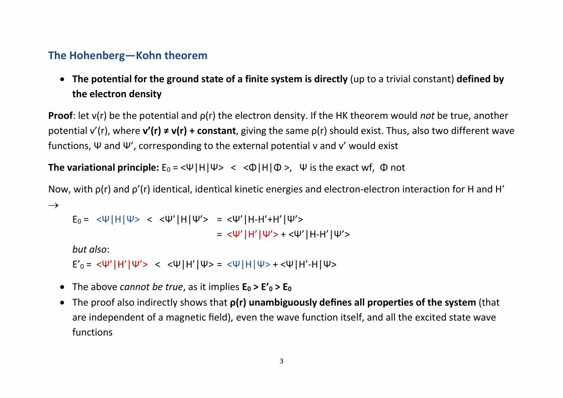
∂ The potential for the ground state of a finite system is directly (up to a trivial constant) defined bythe electron density
Proof: let v(r) be the potential and ρ(r) the electron density. If the HK theorem would not be true, anotherpotential v’(r), where v’(r) ≠ v(r) + constant, giving the same ρ(r) should exist. Thus, also two different wavefunctions, Ψ and Ψ’, corresponding to the external potential v and v’ would exist
The variational principle: E0 = <Ψ|H|Ψ> < <Φ|H|Φ >, Ψ is the exact wf, Φ not
Now, with ρ(r) and ρ’(r) identical, identical kinetic energies and electron-electron interaction for H and H’↑
E0 = <Ψ|H|Ψ> < <Ψ’|H|Ψ’> = <Ψ’|H-H’+H’|Ψ’>= <Ψ’|H’|Ψ’> + <Ψ’|H-H’|Ψ’>
but also:E’0 = <Ψ’|H’|Ψ’> < <Ψ|H’|Ψ> = <Ψ|H|Ψ> + <Ψ|H’-H|Ψ>
∂ The above cannot be true, as it implies E0 > E’0 > E0
∂ The proof also indirectly shows that ρ(r) unambiguously defines all properties of the system (thatare independent of a magnetic field), even the wave function itself, and all the excited state wavefunctions
4
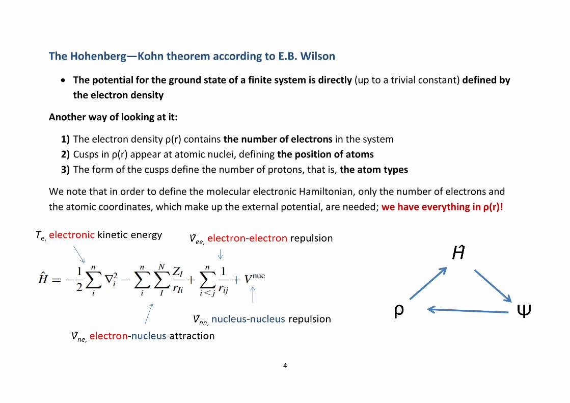
The Hohenberg—Kohn theorem according to E.B. Wilson
∂ The potential for the ground state of a finite system is directly (up to a trivial constant) defined bythe electron density
Another way of looking at it:
1) The electron density ρ(r) contains the number of electrons in the system2) Cusps in ρ(r) appear at atomic nuclei, defining the position of atoms3) The form of the cusps define the number of protons, that is, the atom types
We note that in order to define the molecular electronic Hamiltonian, only the number of electrons andthe atomic coordinates, which make up the external potential, are needed; we have everything in ρ(r)!
5
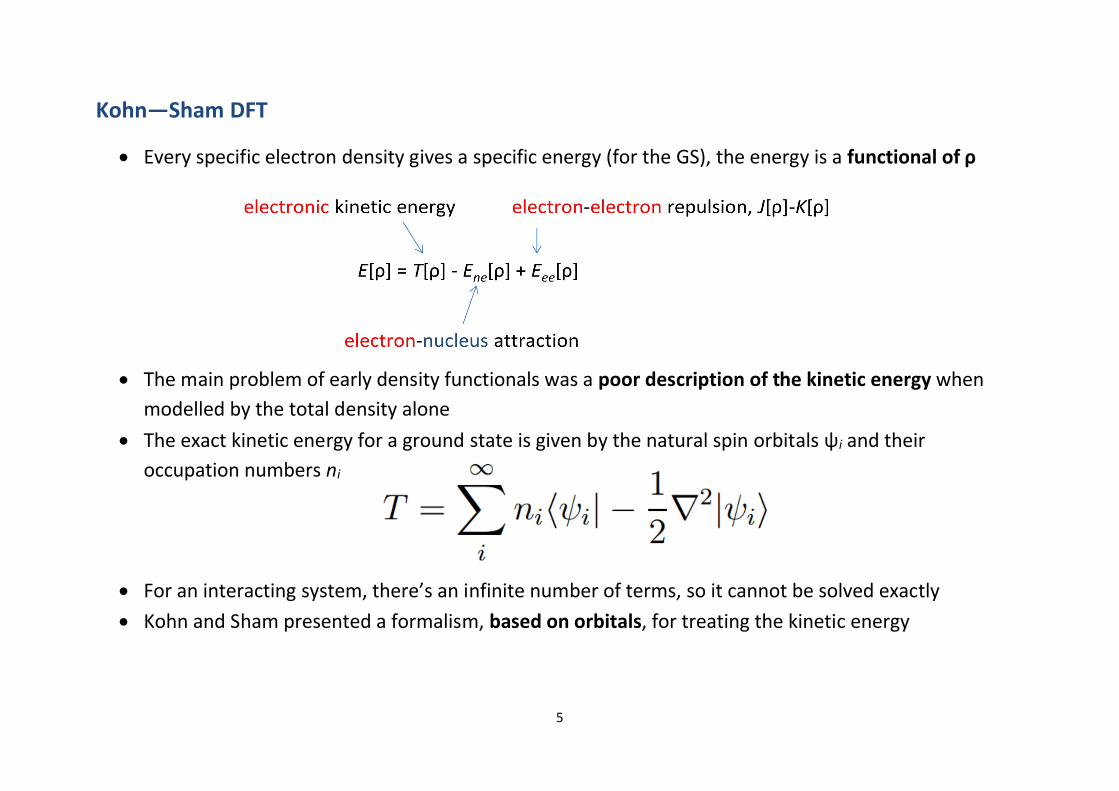
Kohn—Sham DFT
∂ Every specific electron density gives a specific energy (for the GS), the energy is a functional of ρ
∂ The main problem of early density functionals was a poor description of the kinetic energy whenmodelled by the total density alone
∂ The exact kinetic energy for a ground state is given by the natural spin orbitals ψi and theiroccupation numbers ni
∂ For an interacting system, there’s an infinite number of terms, so it cannot be solved exactly∂ Kohn and Sham presented a formalism, based on orbitals, for treating the kinetic energy
6
Kohn—Sham DFT
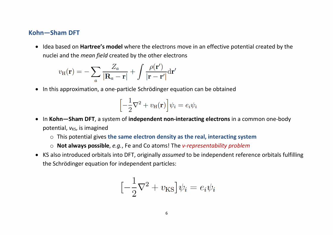
∂ Idea based on Hartree’s model where the electrons move in an effective potential created by thenuclei and the mean field created by the other electrons
∂ In this approximation, a one-particle Schrödinger equation can be obtained
∂ In Kohn—Sham DFT, a system of independent non-interacting electrons in a common one-bodypotential, vKS, is imaginedo This potential gives the same electron density as the real, interacting systemo Not always possible, e.g., Fe and Co atoms! The v-representability problem
∂ KS also introduced orbitals into DFT, originally assumed to be independent reference orbitals fulfillingthe Schrödinger equation for independent particles:
7
Kohn—Sham DFT
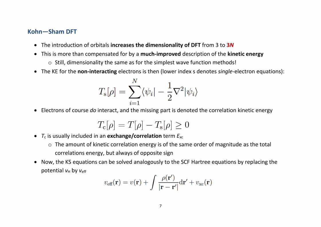
∂ The introduction of orbitals increases the dimensionality of DFT from 3 to 3N∂ This is more than compensated for by a much-improved description of the kinetic energy
o Still, dimensionality the same as for the simplest wave function methods!∂ The KE for the non-interacting electrons is then (lower index s denotes single-electron equations):
∂ Electrons of course do interact, and the missing part is denoted the correlation kinetic energy
∂ Tc is usually included in an exchange/correlation term Exc
o The amount of kinetic correlation energy is of the same order of magnitude as the totalcorrelations energy, but always of opposite sign
∂ Now, the KS equations can be solved analogously to the SCF Hartree equations by replacing thepotential vH by veff
8
Kohn—Sham DFT
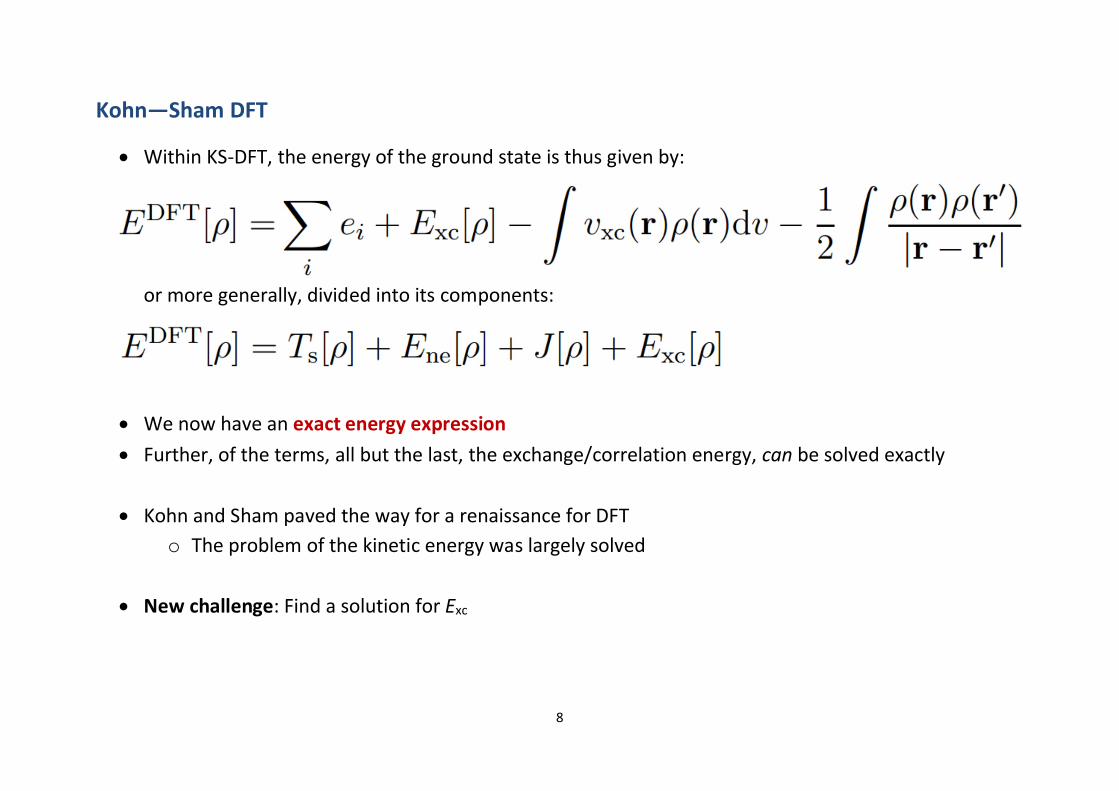
∂ Within KS-DFT, the energy of the ground state is thus given by:
or more generally, divided into its components:
∂ We now have an exact energy expression∂ Further, of the terms, all but the last, the exchange/correlation energy, can be solved exactly
∂ Kohn and Sham paved the way for a renaissance for DFTo The problem of the kinetic energy was largely solved
∂ New challenge: Find a solution for Exc
9
Different DFT models
∂ In wave function theory, there is a systematic way of improving the quality of the modelo Not much joy if the systems are so large that nothing proper can be performed...
∂ Within DFT, the exact functional really is unknowno Some constraints on properties the functional should fulfil are known
∂ Hierarchies of different complexity do exist also within DFT∂ The idea is to include more complex properties of the electron density into the description
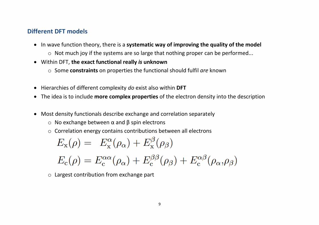
∂ Most density functionals describe exchange and correlation separatelyo No exchange between α and β spin electronso Correlation energy contains contributions between all electrons
o Largest contribution from exchange part

10
The Local Density Approximation (LDA)
∂ Takes only the electron density in specific points in space into account∂ In LDA, the electron density is assumed to vary slowly in space
∂ The exchange energy of a uniform electron gas is analytically known (Slater/Dirac/Bloch exchange)
∂ This is where the train stops for analytically derived DFT∂ There is no known equation for the correlation energy for even such a simple model system as the
uniform electron gas!o It can, however, be computed very accurately using quantum Monte Carlo, and numerical fits to
the results can be formulated∂ The fact remains that already the LDA correlation functionals are nothing but ad hoc functionals with
no real physical meaning except that they provide good results∂ A few different LDA correlation functionals are regularly used
o VWN-3 and VWN-5 by Vosko, Wilk, and Nusairo PW92 by Perdew and Wang

11
Chemically useful approximations
∂ LDA is not accurate enough for chemistryo On rare occasions, it seems to be, but only due to heavy error cancellation
∂ In order to construct more accurate functionals, one notes that ρ(r) contains much more informationthan just the electron density at specific points
∂ Considering increasing amounts of the information contentof the density within the functional form has beendescribed as climbing Jacob’s ladder of DFT, each rungbringing the functional closer to perfectiono Perdew et al,” Some Fundamental Issues in Ground-
State Density Functional Theory: A Guide for thePerplexed”, J. Chem. Theory Comput. 5 (2009) 902,http://dx.doi.org/10.1021/ct800531s
∂ Increased accuracy (usually) comes at a price: Climbing theladder makes the calculations more expensive!

12
The Generalised Gradient Approximation
∂ The electron density is not uniform∂ GGAs account for this by also considering the gradient of the density ∠ρ into account
o Introduced in 1986 by Perdew and Wang; before, gradients had only been considered to secondorder, |∠ρ|2
o Term generalised comes from the GGAs considering higher powers of |∠ρ| into account;generally, any power
∂ A general GGA thus has the form∂ GGAs are semi-local∂ Usually build upon the LDA expressions:
Meta-GGAs
∂ In addition to ρ and ∠ρ, also the Laplacian ∠2ρ and/or the kinetic energy density τ considered
∂ τ depends on the KS orbitals, meta-GGAs that use τ are thus non-local
13
Hybrid functionals
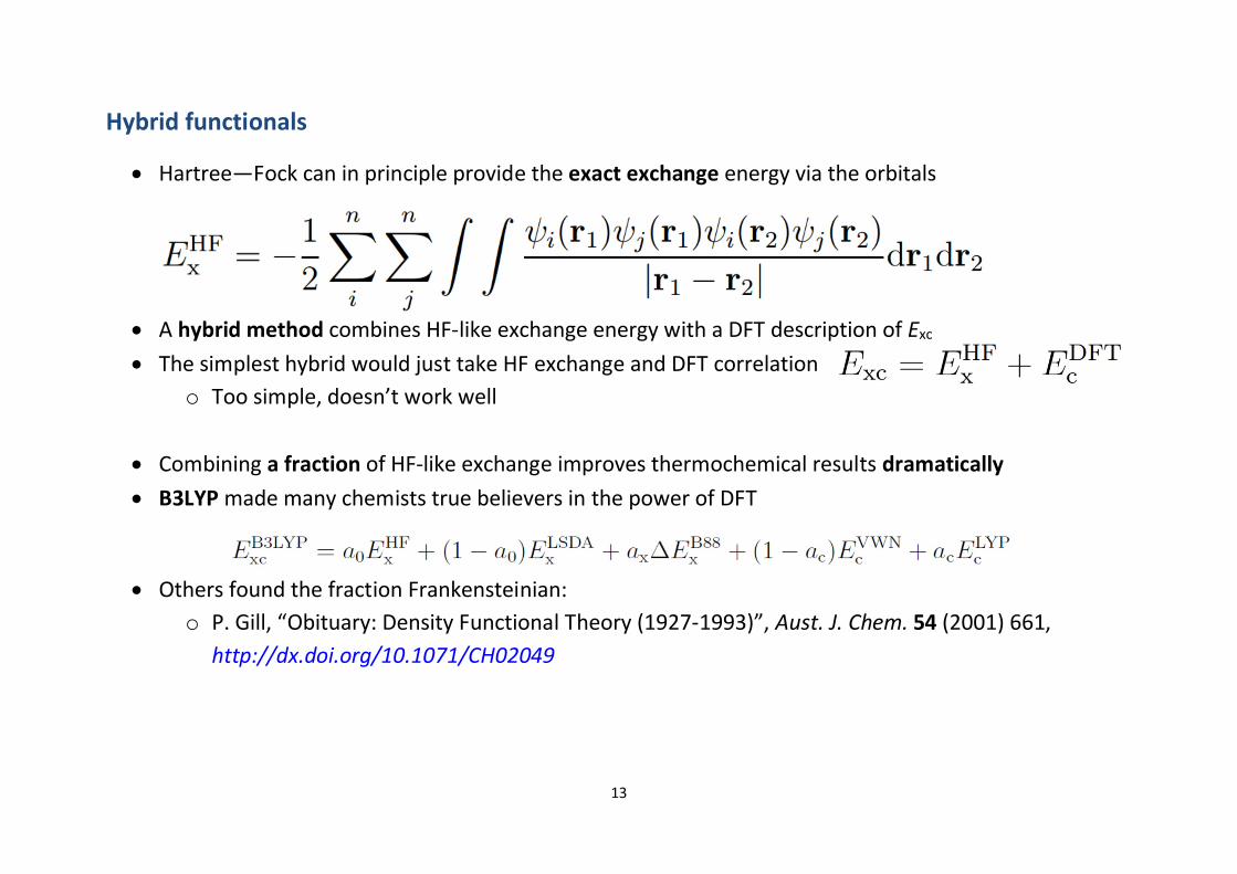
∂ Hartree—Fock can in principle provide the exact exchange energy via the orbitals
∂ A hybrid method combines HF-like exchange energy with a DFT description of Exc
∂ The simplest hybrid would just take HF exchange and DFT correlationo Too simple, doesn’t work well
∂ Combining a fraction of HF-like exchange improves thermochemical results dramatically∂ B3LYP made many chemists true believers in the power of DFT
∂ Others found the fraction Frankensteinian:o P. Gill, “Obituary: Density Functional Theory (1927-1993)”, Aust. J. Chem. 54 (2001) 661,
http://dx.doi.org/10.1071/CH02049

14
Hybrid functionals
∂ A bit of HF-like exchange can be motivated by the adiabatic connection (Harris, PRA 29 (1984) 1648)
∂ λ is an interelectronic coupling-strength parameter that “switches on” the electron—electroninteractiono λ = 0: the non-interacting Kohn—Sham systemo λ = 1: the fully interacting real systemo 0 < λ < 1: intermediately interacting systems
∂ The density is constant through 0 ↑ 1∂ When λ = 0, the exchange-correlation energy is the pure exchange energy of the Slater determinant
of the KS orbitals with no dynamical correlation whatsoever

15
Functional development philosophies functionals
∂ Even with the ingredients of different levels of DFT in place, the actual recipe on how to use them iscompletely open
∂ Different approaches existo Invent a functional form that reproduces wanted data: empiricalo Invent a functional form that fulfils known properties of the true functional: non-empiricalo Use both approaches; often starting from a non-empirical formulation and slightly adjusting it
for pragmatic reasons
∂ Empirical functionals usually work well for systems similar to those parameterised foro Can fail spectacularly when outside their comfort region
∂ Non-empirical functionals usually perform less wello But without parameters for specific systems, can be hoped to perform equally well for
“everything”
16
Non-empirical functionals
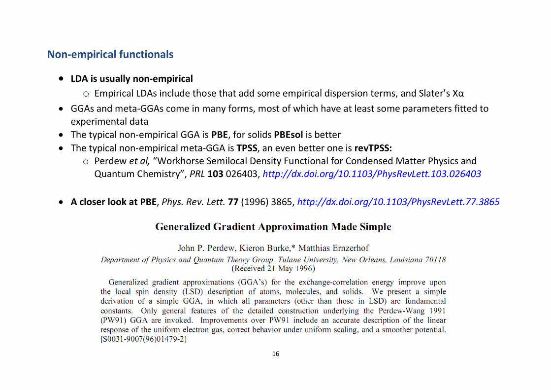
∂ LDA is usually non-empiricalo Empirical LDAs include those that add some empirical dispersion terms, and Slater’s Xα
∂ GGAs and meta-GGAs come in many forms, most of which have at least some parameters fitted toexperimental data
∂ The typical non-empirical GGA is PBE, for solids PBEsol is better∂ The typical non-empirical meta-GGA is TPSS, an even better one is revTPSS:
o Perdew et al, “Workhorse Semilocal Density Functional for Condensed Matter Physics andQuantum Chemistry”, PRL 103 026403, http://dx.doi.org/10.1103/PhysRevLett.103.026403
∂ A closer look at PBE, Phys. Rev. Lett. 77 (1996) 3865, http://dx.doi.org/10.1103/PhysRevLett.77.3865

17
PBE
∂ One motivation for the construction was to simplify the non-empirical PW91 functional, in which theauthors identified the following undesirable features:
1. The derivation is long, and depends on a mass of detail2. The analytic function f is complicated and non-transparent3. f is overparametrized4. The parameters are not seamlessly joined, leading to spurious wiggles in the XC potential δEXC/δρ
which comes with some problems5. PW91 does not behave correctly under uniform scaling to the high-density limit6. It describes linear response of the uniform electron gas less satisfactorily than does LDA
∂ PW91 was constructed to satisfy as many exact conditions as possible∂ The semi-local form of a GGA is however too restrictiveo Fulfilling one exact property can break another!
∂ For PBE, only conditions that were considered energetically important are satisfiedo Less important conditions are ignored
Next up, a quick non-detailed overview of the derivation
18
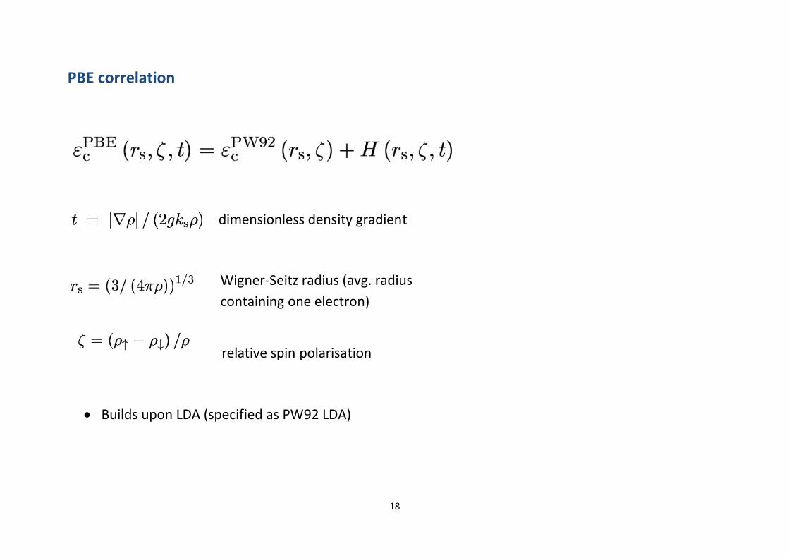
PBE correlation
dimensionless density gradient
Wigner-Seitz radius (avg. radius containing one electron)
relative spin polarisation
∂ Builds upon LDA (specified as PW92 LDA)

19
PBE correlation
∂ Three exact conditions are satisfied
1. In the slowly varying limit (t --> 0), H should go to
2. In the rapidly varying limit (t --> ⁄)
This makes correlation vanish
3. Under uniform scaling, the correlation energy must scale to a constant
To achieve this, H must cancel the logarithmic singularity of εCLDA

20
PBE correlation
∂ All the above three conditions are satisfied by the following form for H:
∂ When t=0, H is exactly condition 1, when t-->⁄, H grows monotonically to the limit of condition 2∂ Thus, EC
GGA ≤ 0

21
PBE correlation
∂ Compared to PW91, quite much simpler:
22
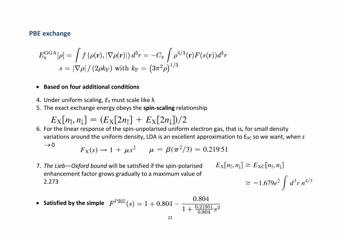
PBE exchange
∂ Based on four additional conditions
4. Under uniform scaling, EX must scale like λ5. The exact exchange energy obeys the spin-scaling relationship
6. For the linear response of the spin-unpolarised uniform electron gas, that is, for small densityvariations around the uniform density, LDA is an excellent approximation to EXC so we want, when s↑ 0
7. The Lieb—Oxford bound will be satisfied if the spin-polarisedenhancement factor grows gradually to a maximum value of2.273
∂ Satisfied by the simple

23
PBE exchange
∂ Again, quite much simpler than PW91:
24
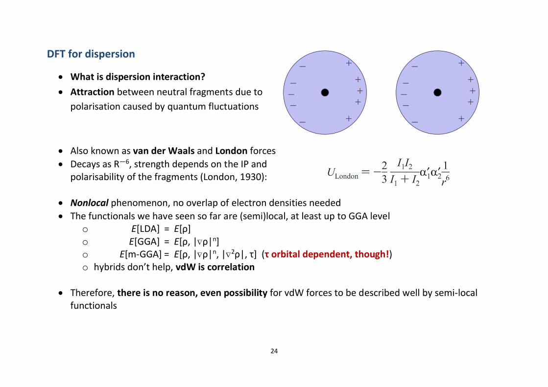
DFT for dispersion
∂ What is dispersion interaction?∂ Attraction between neutral fragments due to
polarisation caused by quantum fluctuations
∂ Also known as van der Waals and London forces∂ Decays as R—6, strength depends on the IP and
polarisability of the fragments (London, 1930):
∂ Nonlocal phenomenon, no overlap of electron densities needed∂ The functionals we have seen so far are (semi)local, at least up to GGA level
o E[LDA] = E[ρ]o E[GGA] = E[ρ, |∠ρ|n]o E[m-GGA] = E[ρ, |∠ρ|n, |∠2ρ|, τ] (τ orbital dependent, though!)o hybrids don’t help, vdW is correlation
∂ Therefore, there is no reason, even possibility for vdW forces to be described well by semi-localfunctionals

25
DFT for dispersion
∂ Attempts to modify (reparametrize) existing functionals∂ X3LYP, Xu and Goddard, PNAS 101 (2004) 2673.
o Was designed for non-covalent interactionso But doesn’t work that well...o ...it shouldn’t
∂ Truhlar et al have designed several Minnesotafunctionalso MPW1B95, MPWB1K, MPWKCIS,
MPWKCIS1K, MPW3LYP, MPWLYP1M,X1B95, XB1K, BB1K, PW6B95, PWB6K, M05,M05-2X, M06, M06-L, M06-HF, M06-2X,M08-HX, M08-SO, ...
o Some of them seem to work well also fornon-covalent interactions, at least some ofthe time, but none are really that well tested(yet)
o Very highly parameterised, very difficult topredict when they fail, but they do fail!

26
DFT for dispersion—B2PLYP∂ Also incorporation of correlated WF methods (MP2) has been used
∂ B2-PLYP, Grimme J. Chem. Phys. 124 (2006) 034108∂ Based on the B88 exchange functional and the LYP correlation functional (BLYP)∂ HF exact exchange added∂ Second order perturbation (PT2/MP2) added
o It is thus a double-hybrid functional

27
DFT for dispersion—B2PLYPo Can also be considered to be on the fifth rung of Jacob’s ladder, as it takes virtual orbitals into
account
One can note from the expression that when
∂ ax = 0; b=1; c=0, B2-PLYP = BLYP∂ ax = 1; b=0; c=1, B2-PLYP = MP2
Final fitted parameters:
ax= 0.57; c = 0.27; b = 1—c = 0.73

28
DFT for dispersion—B2PLYP∂ “Drawbacks” of B2-PLYP compared to “normal” DFT∂ Higher basis set demand
o The virtual space in the PT2 treatment requires larger basis sets, just as normal WF MP2o Minimum recommended: TZVPPo “I would consider an B2PLYP/6-31g* type calculation as almostuseless”, Grimme, CCL 16 Oct 2009
∂ Somewhat larger computational costo Compared to other hybrids, not that bad, as the MP2 term can be computed quite efficiently
with RI (RI-B2-PLYP)
∂ Still not that good for long-range dispersion!o PT2 part relatively small compared to the poorly performing LYP correlation
∂ Overall, seems to work quite well, however

29
Empirical force-field type dispersion on top of DFT: DFT-D
∂ MM force fields can perform much better for dispersion than DFT, at least for dispersion∂ The R—6 term is simply one of the force field parameters
∂ As dispersion is long-range, it usually has a very small effect on the total density∂ This motivates the general form of DFT-D
∂ The dispersion correction is just added on top of the normal DFT calculation
∂ The potential energy surface is thus modified, and better geometries and binding energies shouldthen be obtained
30
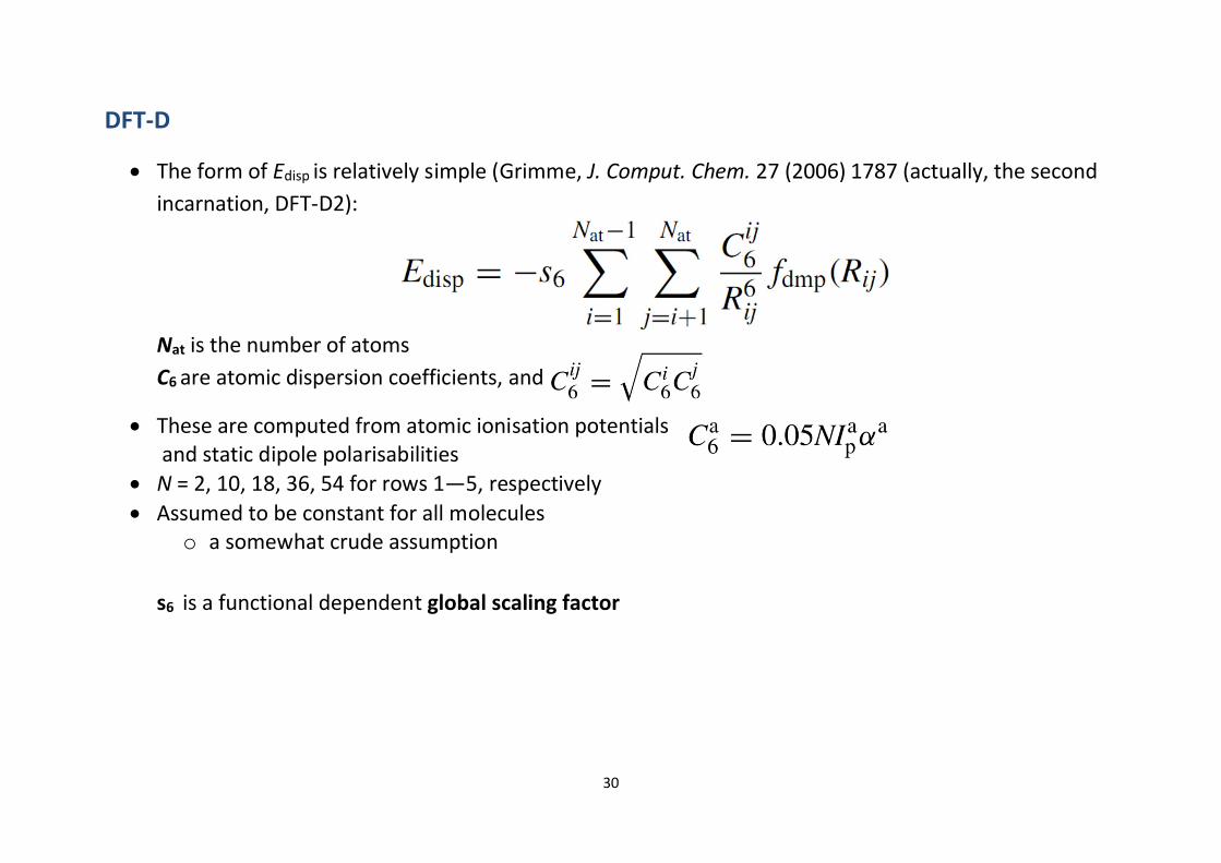
DFT-D
∂ The form of Edisp is relatively simple (Grimme, J. Comput. Chem. 27 (2006) 1787 (actually, the secondincarnation, DFT-D2):
Nat is the number of atomsC6 are atomic dispersion coefficients, and
∂ These are computed from atomic ionisation potentials and static dipole polarisabilities
∂ N = 2, 10, 18, 36, 54 for rows 1—5, respectively∂ Assumed to be constant for all molecules
o a somewhat crude assumption
s6 is a functional dependent global scaling factor
31
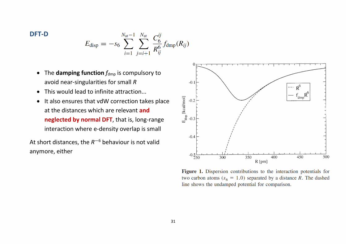
DFT-D
∂ The damping function fdmp is compulsory toavoid near-singularities for small R
∂ This would lead to infinite attraction...∂ It also ensures that vdW correction takes place
at the distances which are relevant andneglected by normal DFT, that is, long-rangeinteraction where e-density overlap is small
At short distances, the R—6 behaviour is not validanymore, either

32
DFT-D
∂ The damping function has the form:
∂ Rr is the sum of the atomic van der Waals radiio These need to be fitted/computed. Assumed to be constant for all moleculesƒ Not as bad as for C6
∂ d is a “sufficiently large” (=20) damping parameter, which switches off the correction at smalldistanceso No correction at small distanceso Some correction at intermediate distanceso Full correction at large distances
∂ The problem of double-counting correlation is still real, even after damping!o “Fixed” by the scaling parameter s6
o s6 is fitted to 40 non-covalently bound complexesƒ PBE: 0.75ƒ BLYP: 1.2ƒ BP86: 1.05ƒ TPSS: 1.0ƒ B3LYP: 1.05ƒ B97-D: 1.25ƒ B2PLYP: 0.55 ↔ dispersion already in via PT2 (note: triple-counting of correlation...)

33
Performance of DFT-D
∂ DFT-D usually works quite well!
Average signed errors for H-bonded, dispersion bonded, and“mixed” interaction energies from the S22 set; BSSEcorrected TZVP, kcal/mol, DFT / DFT-D (J. Comput. Chem. 28(2007) 555)
H-bonded dispersion mixedPBE 0.77 / -0.70 4.90 / 0.52 1.88 / 0.08TPSS 1.45 / -0.23 5.81 / 0.74 2.46 / 0.47B3LYP 1.70 / -0.31 6.56 / 0.87 2.86 / 0.58
BUT: DFT-D is not the final solution!∂ Just as with force fields, it works well for the types ofsystems it was designed for∂ The possible double counting of correlation is ever present∂ There is no way to know exactly what is missing in DFT,and thus adding “something” on top can (will) fail
34
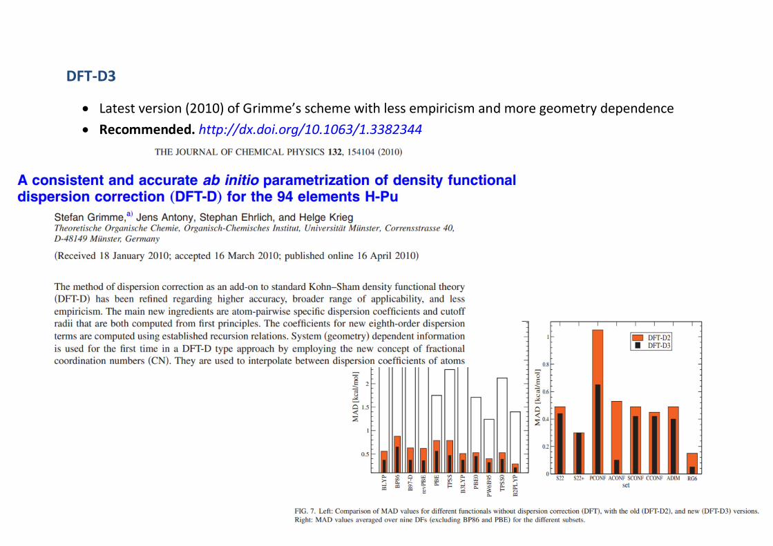
DFT-D3
∂ Latest version (2010) of Grimme’s scheme with less empiricism and more geometry dependence∂ Recommended. http://dx.doi.org/10.1063/1.3382344
35
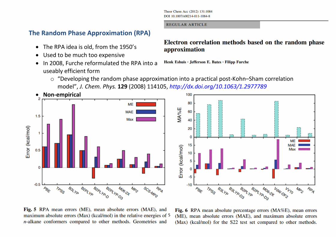
The Random Phase Approximation (RPA)
∂ The RPA idea is old, from the 1950’s∂ Used to be much too expensive∂ In 2008, Furche reformulated the RPA into a
useably efficient formo “Developing the random phase approximation into a practical post-Kohn–Sham correlation
model”, J. Chem. Phys. 129 (2008) 114105, http://dx.doi.org/10.1063/1.2977789∂ Non-empirical

36
Basis sets
∂ Very briefly — What are basis sets∂ Basis sets are used to describe the density distribution in the molecule∂ Within KS-DFT and HF their main use is in describing the molecular orbitals∂ In molecular calculations, they are almost always atom centred∂ Basis sets are composed of a set of functions, which then are populated with the criterion of
minimising the (total) energy∂ For a perfect description (within the model), an infinite amount of different functions would need to
be used∂ The smaller the basis set, the poorer the description (in general)∂ Basis set development has the goal of finding a suitable set of functions that can give a description of
the molecular orbitals as accurately as possible, given a predefined set of functions to choose from∂ In principle, the individual functions could be anything, in practice, they are of Atomic Orbital (AO)
type
37
Basis sets
∂ Two different schemes are in use for describing the functional form of the individual AO’so Slater Type Orbitals (STO’s)o Gaussian Type Orbitals (GTO’s)
∂ GTO’s are most common by far, and almost all basis set development is done within this frameworko The exception is within the ADF community!
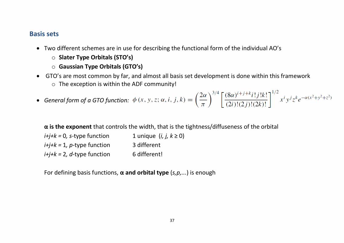
∂ General form of a GTO function:
α is the exponent that controls the width, that is the tightness/diffuseness of the orbitali+j+k = 0, s-type function 1 unique (i, j, k ≥ 0)i+j+k = 1, p-type function 3 differenti+j+k = 2, d-type function 6 different!
For defining basis functions, α and orbital type (s,p,...) is enough
38
Basis set hierarchies
∂ Minimal basis setso Only enough functions to describe the neutral atom
ƒ H and He: 1 s-functionƒ first row: 2 s-functions (1s+2s), one set of p-functions (2px, 2py, 2pz)ƒ etc.
o Not useful for molecules
∂ Double-zeta (DZ) basis setso double the amount of basis functions
ƒ H and He: 2 s-functionƒ first row: 4 s-functions, 2 sets of p-functionsƒ etc.
o Much more useful for moleculeso Able to describe the fact that the electron distribution can be different in different directions

39
Basis set hierarchies
∂ Double-zeta (DZ) basis setso Example: H-C≡N
∂ H—C σ-bond mostly the hydrogen s-orbital + carbon pz-orbital∂ C—N π-bond mostly px and py orbitals of C and N
o more diffuse than the H—C σ-bondo optimal exponent (α) for the C-p orbital smaller in x,y-direction than in the z-direction!o In a minimal basis, they cannot be differento In a DZ basis, they can --> much improved description
∂ Split-valence (SV) basis setso Mostly the valence orbitals are affected by chemical bondingo Core orbitals (e.g., 1s in carbon) stay very much the sameo Thus, doubling the amount of core orbitals is seldom worth the increased costo Most often, a double-zeta basis set is in fact “only” double-zeta in the valence region, sometimes
denoted VDZ, or SV, often simply as double-zeta, anyway
40
Basis set hierarchies
∂ Triple-zeta (TZ), quadruple-zeta (QZ), etc. basis setso Just add more functions for an even better descriptiono Also here, usually only in the valence region
∂ Polarised basis setso In unpolarised basis sets as those above, only functions of the type present in the free atoms
ƒ only s-functions for H; s and p for C, etc.o Higher angular momentum functions, polarisation functions, are almost always important
ƒ p, d, ... for H; d, f, ... for C, etc.
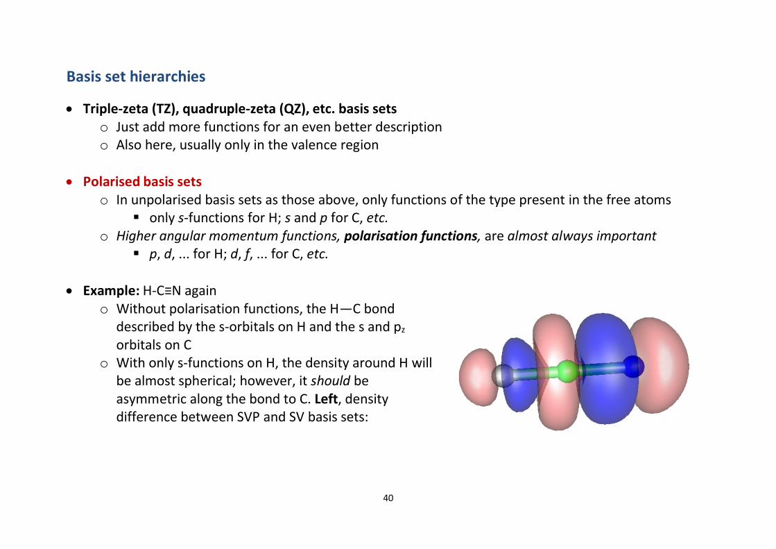
∂ Example: H-C≡N againo Without polarisation functions, the H—C bond
described by the s-orbitals on H and the s and pz
orbitals on Co With only s-functions on H, the density around H will
be almost spherical; however, it should beasymmetric along the bond to C. Left, densitydifference between SVP and SV basis sets:

41
Basis set hierarchies
∂ Polarisation functions are thus very important and should always be used!∂ Basis sets with polarisation functions are denoted in various ways
o 6-31G*, 6-311G**, SVP, TZVPP, cc-pVDZ, ...o confusing nomenclature at best...
∂ Sometimes, one can get away without polarisation functions on hydrogeno SV(P) instead of SVP; 6-31G* instead of 6-31G**
∂ Polarisation functions are usually more important than more freedom in the unpolarised parto DZP more accurate than DZo DZP smaller than TZ, but usually better anyway!
∂ Even a “complete” unpolarised basis set cannot describe bonding properly!
∂ Diffuse basis functionso For anions, highly excited electronic states, loosely bound complexes, the HOMO orbitals are
usually spatially much more diffuse than “normal” orbitalso For describing these systems, it is necessary to add, augment, the basis set with diffuse functions,
functions with very small αo Can also be advantageous when studying transition states, just in order to better describe the
internuclear space when bond distances are longer than at stationary points of the PES.o Nomenclature again somewhat non-standard
∂ 6-31+G(d), aug-cc-pVTZ, aug-TZVP

42
Basis sets for HF, DFT, and correlated WF methods
∂ With HF and DFT, moderately sized basis sets are usually sufficient to get results close to the basis setlimito Much smaller than correlated wave function methodso Comparable to that of Hartree—Fock
∂ Most of the older basis sets have not been optimised for DFT
∂ Correlated WF methods, on the other hand, require very large basis setso Slow convergence of the correlation energy wrt angular momentum
∂ Also, special basis sets needed for correlating core electronso Most basis sets are not designed for this, and will give an unbalanced description of core—core
and core—valence correlation∂ With standard basis sets, the core electrons must be frozen, uncorrelated
o Sometimes one sees calculations specified as MP2/full, 6-31G*o Usually indicates that the authors don’t know what they are doing
43
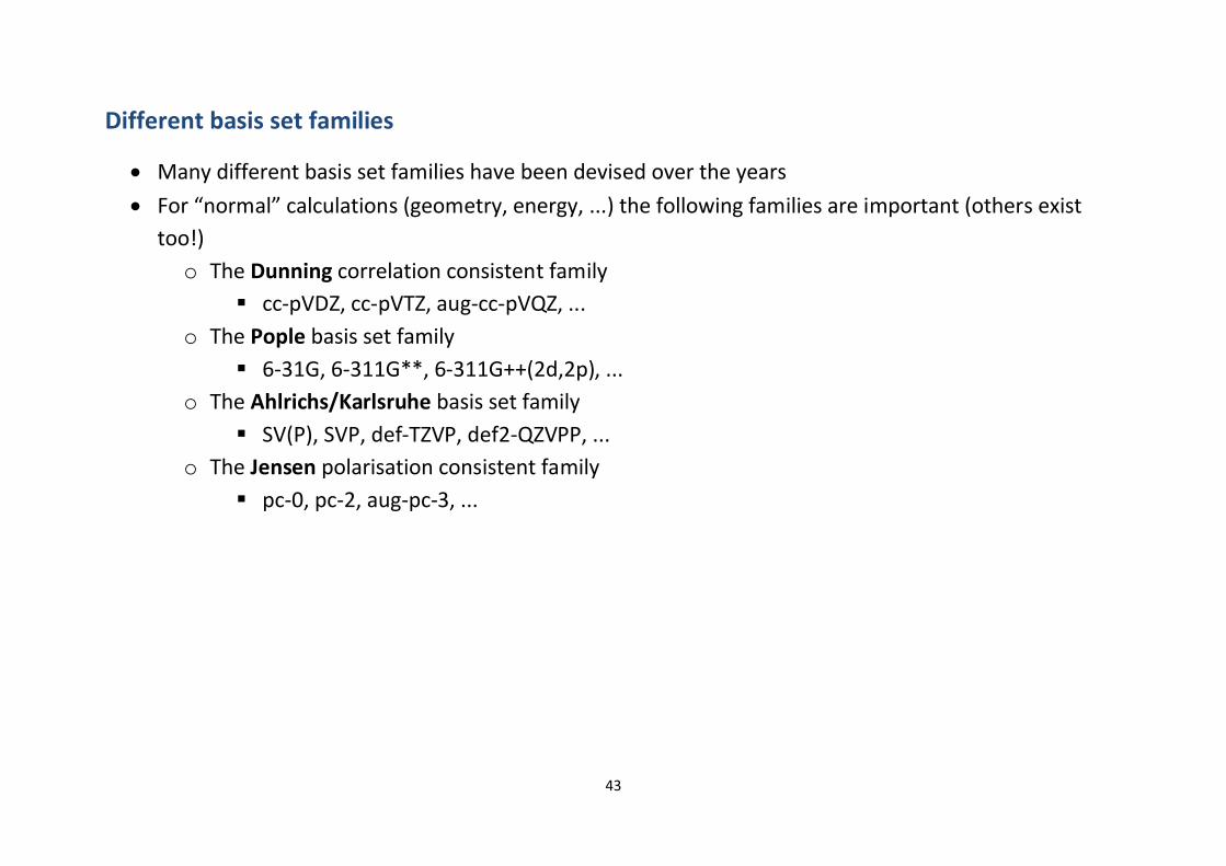
Different basis set families
∂ Many different basis set families have been devised over the years∂ For “normal” calculations (geometry, energy, ...) the following families are important (others exist
too!)o The Dunning correlation consistent family
ƒ cc-pVDZ, cc-pVTZ, aug-cc-pVQZ, ...o The Pople basis set family
ƒ 6-31G, 6-311G**, 6-311G++(2d,2p), ...o The Ahlrichs/Karlsruhe basis set family
ƒ SV(P), SVP, def-TZVP, def2-QZVPP, ...o The Jensen polarisation consistent family
ƒ pc-0, pc-2, aug-pc-3, ...
44
Different basis set families
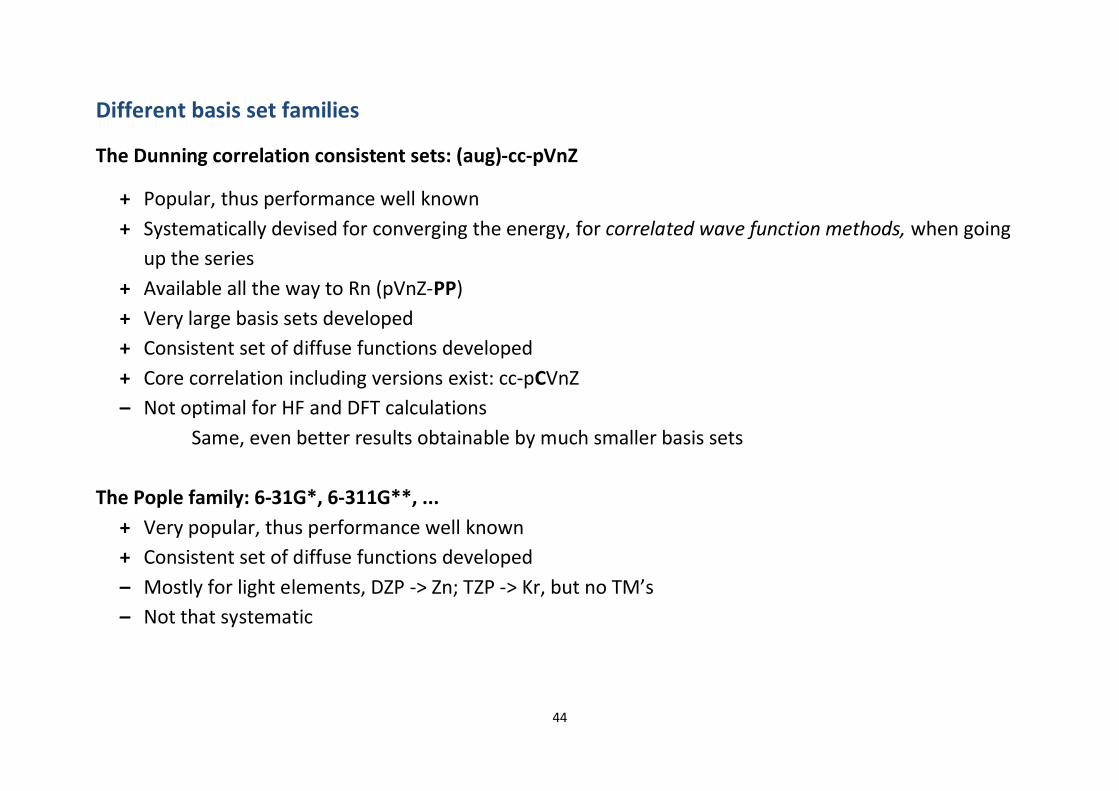
The Dunning correlation consistent sets: (aug)-cc-pVnZ
+ Popular, thus performance well known+ Systematically devised for converging the energy, for correlated wave function methods, when going
up the series+ Available all the way to Rn (pVnZ-PP)+ Very large basis sets developed+ Consistent set of diffuse functions developed+ Core correlation including versions exist: cc-pCVnZ– Not optimal for HF and DFT calculations
Same, even better results obtainable by much smaller basis sets
The Pople family: 6-31G*, 6-311G**, ...+ Very popular, thus performance well known+ Consistent set of diffuse functions developed– Mostly for light elements, DZP -> Zn; TZP -> Kr, but no TM’s– Not that systematic

45
Different basis set families
The Ahlrichs/Karlsruhe family: SVP, def-TZVP, def2-QZVPP, ...+ Quite efficient for HF and DFT, more so than Pople’s+ QZP quality for all elements up to Rn+ Recently augmented by diffuse functions, def2-TZVPD, etc.+ The doubly polarised versions starting from def2-TZVPP also OK for MP2, CC2, etc.– Not very systematic naming
Energy convergence also somewhat erratic
Jensen’s polarisation consistent family: pc-0, aug-pc-1, ...+ Optimised for DFT (and HF) calculations+ Systematic convergence towards basis set limit, systematic naming+ Consistent set of diffuse functions developed+ Corresponding pcJ-n basis sets for spin—spin coupling constants, pcSseg-n for magnetic shieldings– Computationally more expensive than Karslruhe basis sets Partly because of the general contraction scheme —> recently, pcs-n basis sets!
http://dx.doi.org/10.1021/ct401026a– So far only for the first three rows, including the transition metals

46
Basis set extrapolation—SCF
∂ Basis set extrapolation can be used to estimate the SCF energy at the limit of a Complete Basis Set(CBS)
∂ One formula that has been shown to work well (in connection with Jensen’s pc-n basis sets); requirescalculations with three basis sets of increasing size, and numerical fitting
Lmax = highest angular momentum of the basis set
∂ With DFT and HF, the gain of extrapolation mainly lies in checking for basis-set convergenceo With a large (QZP) basis set, the errors inherent in the methods will always be larger!
47
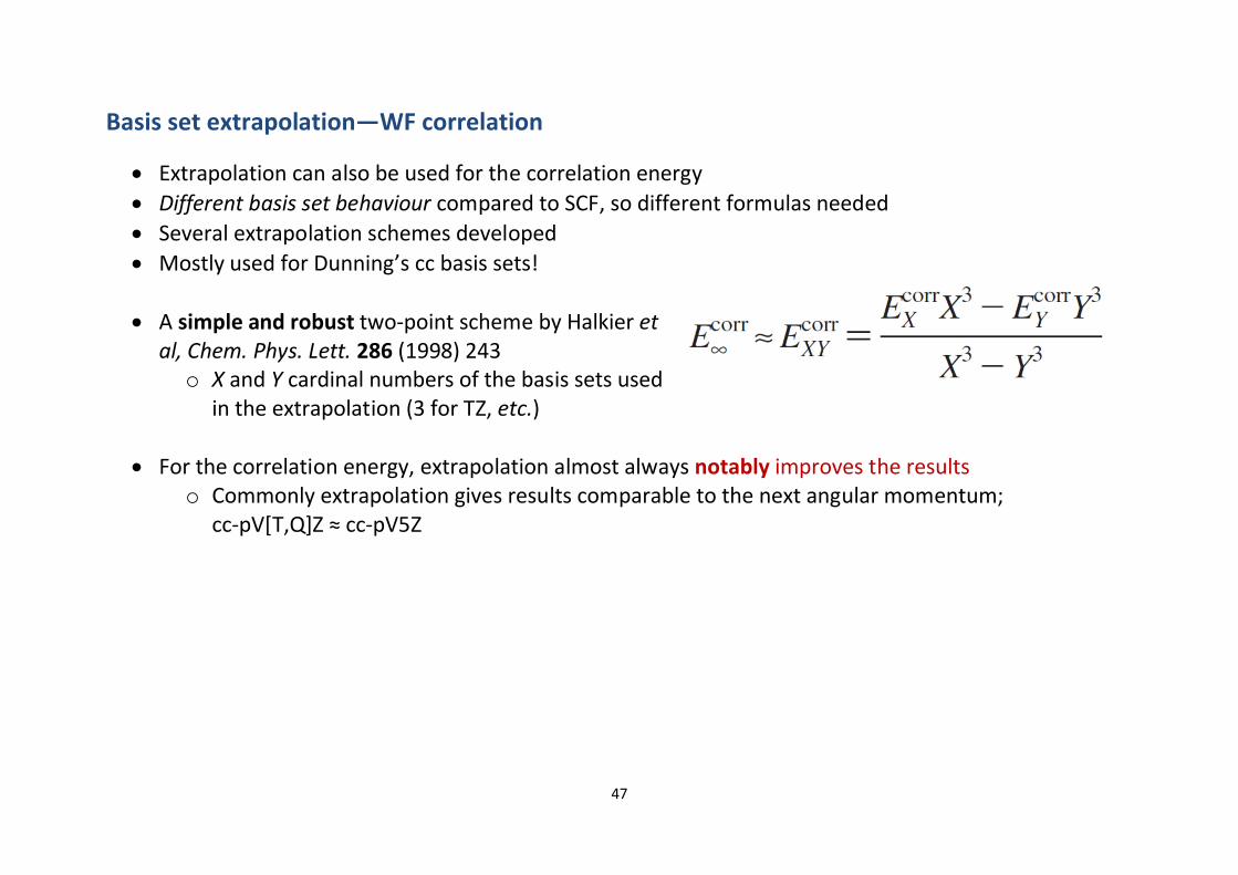
Basis set extrapolation—WF correlation
∂ Extrapolation can also be used for the correlation energy∂ Different basis set behaviour compared to SCF, so different formulas needed∂ Several extrapolation schemes developed∂ Mostly used for Dunning’s cc basis sets!
∂ A simple and robust two-point scheme by Halkier etal, Chem. Phys. Lett. 286 (1998) 243o X and Y cardinal numbers of the basis sets used
in the extrapolation (3 for TZ, etc.)
∂ For the correlation energy, extrapolation almost always notably improves the resultso Commonly extrapolation gives results comparable to the next angular momentum;
cc-pV[T,Q]Z ≈ cc-pV5Z

48
Further reading
∂ The surface was barely scratched∂ For more details, the following text books are excellent
∂ Frank Jensen, “Introduction to Computational Chemistry”o Nice overview of QC methods, as well as the basics of MM
∂ Wolfram Koch, Max C. Holthausen, “A Chemist’s Guide to Density Functional Theory”o Fundamentals of DFT from a chemical viewpoint
∂ Kieron Burke et al, “The ABC of DFT”, http://dft.uci.edu/research.phpo A modern more in-depth treatment of DFT. Preliminary version but already good
∂ Trygve Helgaker, Poul Jørgensen, Jeppe Olsen, “Molecular Electronic-Structure Theory”o Very detailed account of correlated wave-function methods
∂ Steven M. Bachrach, “Computational Organic Chemistry”o Brief intro of methods, followed by examples relevant for organic chemistry
Good luck!