CSCI 256

Data Structures and Algorithm Analysis

Lecture 18

Some slides by Kevin Wayne copyright 2005, Pearson Addison Wesley all rights reserved, and some by Iker Gondra

Network Flow

Soviet Rail Network, 1955

Reference: On the history of the transportation and maximum flow problems. Alexander Schrijver in Math Programming, 91: 3, 2002.

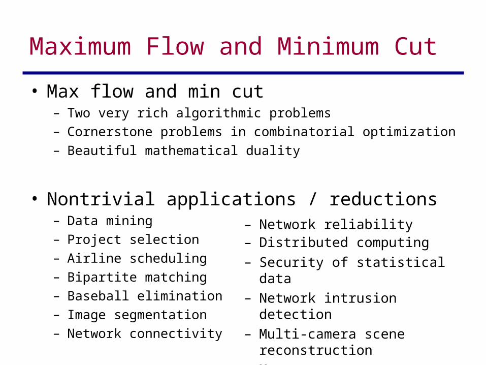
Maximum Flow and Minimum Cut

• Max flow and min cut– Two very rich algorithmic problems– Cornerstone problems in combinatorial optimization– Beautiful mathematical duality

• Nontrivial applications / reductions– Data mining– Project selection– Airline scheduling– Bipartite matching– Baseball elimination– Image segmentation– Network connectivity

– Network reliability– Distributed computing

– Security of statistical data– Network intrusion detection– Multi-camera scene reconstruction– Many many more . . .

Flow Network

• Flow network– Abstraction for material flowing through the edges– G = (V, E) = directed graph, no parallel edges– Two distinguished nodes: s = source, t = sink– c(e) = capacity of edge e

s

2

3

4

5

6

7

t

15

5

30

15

10

8

15

9

6 10

10

10 15 4

4

capacity

source sink

Flows

• Def: An s-t flow is a function that satisfies– For each e E: (capacity)– For each v V – {s, t}: (conservation)

• Def: The value of a flow f is:

• The maximum-flow problem– Given a flow network, a natural goal is to arrange the traffic so

as to make as efficient use as possible of the available capacity– Thus basic algorithmic problem is: given a flow network, find a

flow of maximum possible value

0 f (e) c(e)

f (e)e in to v f (e)

e out of v

v( f ) f (e) e out of s

.

Flow Example

a

s

d

b

c f

e

g

h

i

t

20

5

20 20

20

20

20

55

520

5 10

20

5

20

20

5

20

20

5

5

10

30

How to solve the Max-Flow Problem??

• There is no known algorithm for the Maximum-Flow problem that can be viewed as belonging to the DP paradigm

• What about greedy approaches??• Let us look at a simple example

Simple Flow Example

u

s t

v

20

20

30

10

10

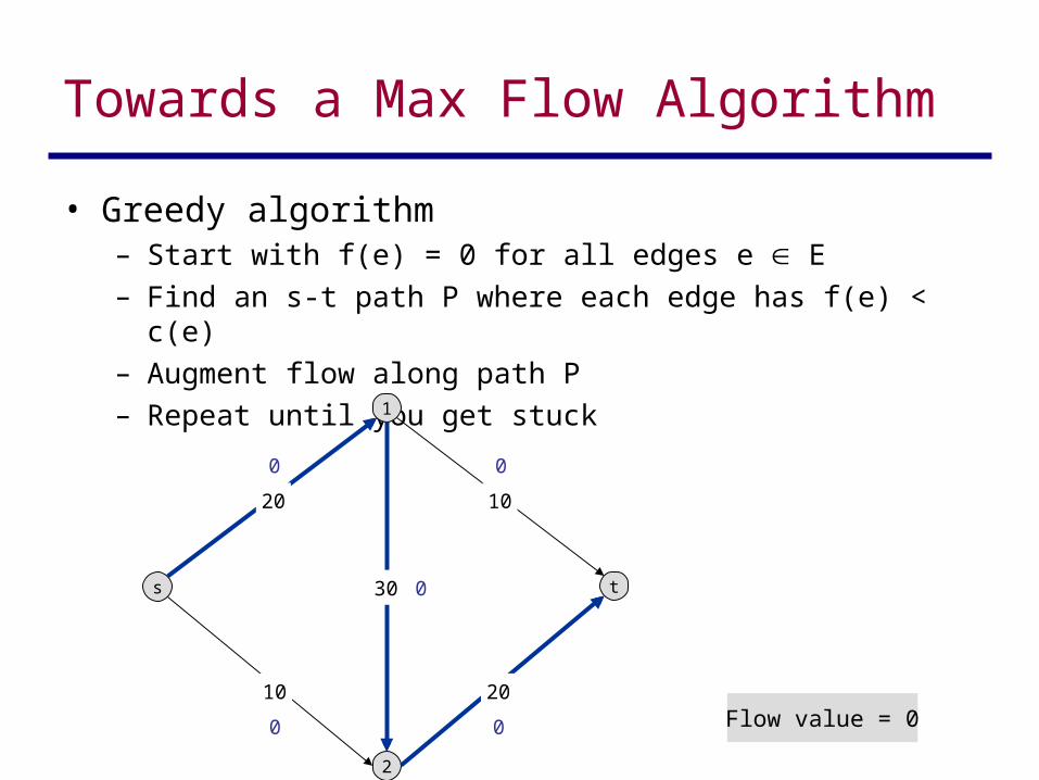
Towards a Max Flow Algorithm

• Greedy algorithm– Start with f(e) = 0 for all edges e E– Find an s-t path P where each edge has f(e) < c(e)– Augment flow along path P– Repeat until you get stuck

s

1

2

t

10

10

0 0

0 0

0

20

20

30

Flow value = 0

Towards a Max Flow Algorithm

• Greedy algorithm– Start with f(e) = 0 for all edge e E– Find an s-t path P where each edge has f(e) < c(e)– Augment flow along path P– Repeat until you get stuck

s

1

2

t

20

Flow value = 20

10

10 20

30

0 0

0 0

0

X

X

X

20

20

20

Towards a Max Flow Algorithm

• Greedy algorithm– Start with f(e) = 0 for all edge e E– Find an s-t path P where each edge has f(e) < c(e)– Augment flow along path P– Repeat until you get stuck

local optimality global optimality

greedy = 20

s

1

2

t

20 10

10 20

30

20 0

0

20

20

opt = 30

s

1

2

t

20 10

10 20

30

20 10

10

10

20

Towards a Max Flow Algorithm

• The way we are going to increase the flow is by finding augmenting paths (i.e., s-t paths that increase the flow)

• The other way that we can increase the flow is by reversing the direction of flow

• Push forward on edges with leftover capacity and push backward on edges that are already carrying flow to divert it in a different direction

• To search for forward-backward capacity for a flow network G and a flow f on G define the notion of residual graph Gf

Residual Graph Gf has original nodes of G = (V,E), and but we redefine the set of edges and their capacities

• Original edge: e = (u, v) E

Given: flow f(e), capacity c(e)

• Gf - Forward edge–(u,v) E, where c(e) > f(e)

• Gf - Backward edge–"Undo" flowsent– eR = (v, u) if f(e) > 0

•- Gf - Capacity:

–For e: it is c(e)-f(e)–For eR : it is f(e)

• Residual graph: Gf = (V, Ef )

–Ef = {e : f(e) < c(e)} {eR : f(e) > 0}

u v 17

6

capacity

flow

u v 11

residual capacity

6

residual capacity

Residual Graph

– Any edge e such that f(e) < c(e) is called a forward edge and edge eR (such that f(e) > 0) is called a backward edge

– Consider our example graph with path s,1,2,t, and flows e(s,1) = 20, e(1,2) = 20 and e(2,t) = 20 and the other edges have 0 flow.

Below, the flow function f is indicated by blue. Build Residual Graph Gf - do in class (see text fig 7.4 (b) )

s

1

2

t

20 10

10 20

30

20 0

0

20

20

To push flow from s to t in Gf

• Call capacities in Gf “residual capacities”

• Let P be a simple s-t path in Gf

• Bottleneck (P,f) = the minimal residual capacity of any edge in P, with respect to f; denote it by b

• b units of flow can be added (to each edge) along the path P

• The following operation augment(f,P) yields a new flow f’ in G:

Augmenting Paths in a Residual Graph

augment(f,P)

Let b = bottleneck(P,f)

For each edge (u,v) in P

If e=(u,v) is a forward edge then

increase f(e) in G by b

Else (u,v) is a backward edge; let e = (v,u)

decrease f(e) in G by b

EndIf

EndFor

Return(f)

example

The algorithm augment(f,P) results in a new flow f’ in G, obtained by increasing and decreasing the flow on edge values of P

Start with f(e) = 0 everywhere. Then Gf = G.

Consider first (simple) path P: s,1, t.

Let f’=augment (P,f); and find Gf’

Then in our example with a new path simple P, the path s,2,1,t in Gf’, find f’’= augment(f’,P) and find Gf’’

Max-Flow Ford Fulkerson Algorithm

Initially f(e) = 0 for all e in G

While there is an s-t path in Gf

Find P a simple s-t path in Gf

f’=augment(P,f)

Update the residual graph Gf to be Gf’

Let f’ be f and Gf’ be Gf

EndWhile

Return f