CSC384: Introduction to Artificial Intelligencefbacchus/csc384/Lectures/csc384-Lecture04-Ga… · CSC384: Introduction to Artificial Intelligence Game Tree Search • Chapter 5.1,

CSC384: Introduction to Artificial Intelligence

Game Tree Search

• Chapter 5.1, 5.2, 5.3, 5.6 cover some of the material we cover here Section 5 6 has an interesting overview of cover here. Section 5.6 has an interesting overview of State-of-the-Art game playing programs.

• Section 5.5 extends the ideas to games with uncertainty (We won’t cover that material but it makes for interesting reading)for interesting reading).

1Fahiem Bacchus, CSC384 Introduction to Artificial Intelligence, University of Toronto

Generalizing Search Problem

• So far: our search problems have assumed agent has complete control of environmentcomplete control of environment• State does not change unless the agent (robot) changes it.

• All we need to compute is a single path to a goal state.

• Assumption not always reasonable• Stochastic environment (e.g., the weather, traffic accidents). • Other agents whose interests conflict with yours

• Search can find a path to a goal state, but the actions might not lead you to the goal as the state can be changed by other agents (nature or other intelligent agents)


Generalizing Search Problem

•We need to generalize our view of search to handle state changes that are not in the control of handle state changes that are not in the control of the agent.

•One generalization yields game tree search• Agent and some other agents.• The other agents are acting to maximize their profits

• this might not have a positive effect on your profits.


General Games

•What makes something a game?Th t ( ) t ki h t • There are two (or more) agents making changes to the world (the state)

• Each agent has their own interestsEach agent has their own interests• e.g., each agent has a different goal; or assigns different costs

to different paths/states• Each agent tries to alter the world so as to best • Each agent tries to alter the world so as to best

benefit itself.


General Games

• What makes games hard?• How you should play depends on how you think the y p y p y

other person will play; but how they play depends on how they think you will play; so how you should play depends on how you think they think you will play; depends on how you think they think you will play; but how they play should depend on how they think you think they think you will play; …


Properties of Games considered here

•Zero-sum games: Fully competitive• Competitive: if one play wins, the others lose;p p y , ;

e.g. Poker – you win what the other player lose• Games can also be cooperative: some

outcomes are preferred by both of us, or at least our values aren’t diametrically opposed

D t i i ti h i l d •Deterministic: no chance involved • (no dice, or random deals of cards, or coin flips,

etc etc. •Perfect information (all aspects of the state

are fully observable e g no hidden cards)


are fully observable, e.g., no hidden cards)

Our Focus: Two‐Player Zero‐Sum Games

•Fully competitive two player games• If you win, the other player (opponent) loses• Zero-sum means the sum of your and your

opponent’s payoff is zero---any thing you gain come at your opponent’s cost (and vice-versa). y pp ( )• Key insight: How you act depends on how the other

agent acts (or how you think they will act)• and vice versa (if your opponent acts rational)• and vice versa (if your opponent acts rational)

•Examples of two-person zero-sum games: • Chess checkers tic-tac-toe backgammon go Chess, checkers, tic tac toe, backgammon, go,

Doom, “find the last parking space”•Most of the ideas extend to multiplayer zero-

( f Ch t 5 2 2)7Fahiem Bacchus, CSC384 Introduction to Artificial Intelligence, University of Toronto

sum games (cf. Chapter 5.2.2)

Game 1: Rock, Paper, Scissors

• Scissors cut paper, paper covers rock, rock smashes scissors

• Represented as a matrix: Player I chooses a row, Player II chooses a column R P S

Player IIa column

• Payoff to each player in each cell (Pl I / Pl II)

R P S

0/0 -1/1 1/-1R

Icell (Pl.I / Pl.II)

• 1: win, 0: tie, -1: loss• so it’s zero-sum

0/0 -1/11/-1P

Play

er

• so it s zero-sum0/0-1/1 1/-1S


Game 2: Prisoner’s Dilemma

• Two prisoner’s in separate cells, sheriff doesn’t have enough evidence to convict them. They agree ahead of time to both deny the crime (they will cooperate).

• If one defects (i.e., confesses) and the other Coop Def( , )doesn’t• confessor goes free• other sentenced to 4 years

3/3 0/4Coopy

• If both defect (confess)• both sentenced to 3 years

• If both cooperate (neither confesses)

1/14/0Def

• If both cooperate (neither confesses) • both sentenced to 1 year on minor charge

P ff 4 i t


• Payoff: 4 minus sentence

Extensive Form Two‐Player Zero‐Sum Games

• Key point of previous games: what you should do depends on what other guy does

• But previous games are simple “one shot” games• single move eachg• in game theory: strategic or normal form games

• Many games extend over multiple movesMany games extend over multiple moves• turn-taking: players act alternatively• e.g., chess, checkers, etc.• in game theory: extensive form gamesg y g

• We’ll focus on the extensive form• that’s where the computational questions emerge


that s where the computational questions emerge

Two‐Player Zero‐Sum Game – Definition

• Two players A (Max) and B (Min)

• Set of positions P (states of the game)• Set of positions P (states of the game)

• A starting position s P (where game begins)

• Terminal positions T P (where game can end)• Terminal positions T P (where game can end)

• Set of directed edges EA between states (A’s moves)• set of directed edges EB between states (B’s moves)

• Utility or payoff function U : T → (how good is each terminal state for player A)

• Why don’t we need a utility function for B?


Two‐Player Zero‐Sum Game – Intuition

• Players alternate moves (starting with Max)• Game ends when some terminal p T is reached

• A game state: a state-player pair• Tells us what state we’re in and whose move it is

• Utility function and terminals replace goals• Max wants to maximize the terminal payoff• Min wants to minimize the terminal payoff

• Think of it as:• Max gets U(t), Min gets –U(t) for terminal node t• This is why it’s called zero (or constant) sum


Tic Tac Toe States

Turn=Max(X) Turn=Max(X)Turn=Min(O)

X X XX X XO

Min(O) Max(X)

O

Min(O) Max(X)

XXO

X XX

XOOO

O

XO

O


U = -1U = +1

Tic Tac Toe Game Tree

Max

X XXMin XMin

X X XO OOMax

Min

XX

OO

O

Min


XX

OX

Game Tree

• Game tree looks like a search tree• Layers reflect alternating moves between A and By g• The search tree in game playing is a subtree of the game tree

• Player A doesn’t decide where to go aloneAft A t t t B d id hi h f th t t hild • After A moves to a state, B decides which of the states children to move to

• Thus A must have a strategy• Must know what to do for each possible move of B• One sequence of moves will not suffice: “What to do” will

depend on how B will playp p y

• What is a reasonable strategy?


Minimax Strategy

• Assume that the other player will always play their best move,• you always play a move that will minimize the payoff that could

be gained by the other player. • My minimizing the other player’s payoff you maximize yours My minimizing the other player s payoff you maximize yours.

• If however you know that Min will play poorly in some circumstances, there might be a better , gstrategy than MiniMax (i.e., a strategy that gives you a better payoff).

• But in the absence of that knowledge minimax


“plays it safe”

Minimax Strategy payoffs

s0 max node

s1 s2 s3

min node

terminal

t1 t2 t3 t4 t5 t6 t7

s1 s2 s3

t1 t2 t3 t4 t5 t6 t77 -6 4 3 9 -10 2

The terminal nodes have utilities.But we can compute a “utility” for the non-terminalstates, by assuming both players always play their


best move.

Minimax Strategy – Intuitions

s0 max node

i d

s1 s2 s3

min node

terminal

t1 t2 t3 t4 t5 t6 t77 -6 4 3 9 -10 2

If Max goes to s1 Min goes to t2 U(s1) = min{U(t1) U(t2) U(t3)} = 6If Max goes to s1, Min goes to t2, U(s1) = min{U(t1), U(t2), U(t3)} = -6If Max goes to s2, Min goes to t4, U(s2) = min{U(t4), U(t5)} = 3If Max goes to s3, Min goes to t6, U(s3) = min{U(t6), U(t7)} = -10


So Max goes to s2: so U(s0) = max{U(s1), U(s2), U(s3)} = 3

Minimax Strategy

• Build full game tree (all leaves are terminals)• Root is start state, edges are possible moves, etc., g p ,• Label terminal nodes with utilities

• Back values up the tree• U(t) is defined for all terminals (part of input)• U(n) = min {U(c) : c is a child of n} if n is a Min nodeU( ) {U(c) : c s a c d o } s a ode• U(n) = max {U(c) : c is a child of n} if n is a Max node


Minimax Strategy

• The values labeling each state are the values that Max will achieve in that state if both Max and Min play their p ybest moves.• Max plays a move to change the state to the highest valued

min childmin child.• Min plays a move to change the state to the lowest valued max

child.If Min plays poorly Max could do better but never • If Min plays poorly, Max could do better, but never worse. • If Max, however knows that Min will play poorly, there might be a

better strategy of play for Max than Minimax.


Depth‐First Implementation of Minimax

• Building the entire game tree and backing up values gives each player their strategy.

• However, the game tree is exponential in size. o e e , e ga e ee s e po e a s e. • Furthermore, as we will see later it is not necessary to know all of

the tree.

• To solve these problems we find a depth-first implementation of minimax.

We run the depth-first search after each move to compute what is the next move for the MAX player. (We could do the same for the MIN player). p y )

• This avoids explicitly representing the exponentially sized game tree: we just compute each move as it is needed.



DFMiniMax(n, Player) //return Utility of state n given that //Player is MIN or MAX

If n is TERMINALIf n is TERMINALReturn U(n) //Return terminal states utility

//(U is specified as part of game)

//Apply Player’s moves to get//Apply Player’s moves to get//successor states.

ChildList = n.Successors(Player) If Player == MINyreturn minimum of DFMiniMax(c, MAX) over c ChildList

Else //Player is MAXreturn maximum of DFMiniMax(c, MIN) over c ChildList



• Notice that the game tree has to have finite depth for this to workthis to work

• Advantage of DF implementation: space efficientg p p

• Minimax will expand O(bd) states, which is both a BEST d WORSE i and WORSE case scenario.

• We must traverse the entire search tree to evaluate all options• We can’t be lucky as in regular search and find a path to a goal y g p g

before searching the entire tree.


Visualization of Depth‐First Minimax

s0Once s17 eval’d, no need to storetree: s16 only needs its value.Once s24 value computed, we can

s1 s13 s16

p ,evaluate s16

s2 6 s17 s24s2 s6 s17 s24

2118

t14 t15

t3 t4 t5 t25 t26s21s18s10s7


t11 t12 t22 t23t19 t20t8 t9

Example

Max

Max

Min

Min

Max

MinMin


Pruning

• It is not necessary to examine entire tree to make correct Minimax decisioncorrect Minimax decision

• Assume depth-first generation of tree• After generating value for only some of n’s children we can

prove that we’ll never reach n in a Minmax strategy.• So we needn’t generate or evaluate any further children of n!

• Two types of pruning (cuts):Two types of pruning (cuts):• pruning of max nodes (α-cuts)• pruning of min nodes (β-cuts)


Cutting Max Nodes (Alpha Cuts)

• At a Max node n:• Let β be the lowest value of n’s siblings examined so far (siblings

to the left of n that have already been searched)• Let α be the highest value of n’s children examined so far

(changes as children examined)

max node

s0

max nodemin nodeterminal

s1 s13 s16

s2 s6

5β =5 only one sibling value known Sequence of values for α as s6’s children are explored:


α =8T38

T410

T55

pα =8 α=10 α=10α =8 α=10

Cutting Max Nodes (Alpha Cuts)

• If α becomes ≥ β we can stop expanding the children of n• Min will never choose to move from n’s parent to n since it

would choose one of n’s lower valued siblings first.

i d

P β = 8

min node

n14 12 8 α = 2 4 9n14 12 8 α = 2 4 9


s1 s2 s32 4 9

Cutting Min Nodes (Beta Cuts)

• At a Min node n:• Let β be the lowest value of n’s children examined so far

( h hild i d)(changes as children examined)• Let α be the highest value of n’s sibling’s examined so far

(fixed when evaluating n)

s0

max nodemin nodet i l

s1 s13 s16terminal

s2 s6α =10

β 5 β 3


β =5 β =3

Cutting Min Nodes (Beta Cuts)

• If β becomes ≤ α we can stop expanding the children of n.• Max will never choose to move from n’s parent to n since it

would choose one of n’s higher value siblings first.

P α = 7

n6 2 7 β = 9 8 3

s1 s2 s3


s1 s2 s39 8 3

Implementing Alpha‐Beta Pruning

AlphaBeta(n,Player,alpha,beta) //return Utility of state If n is TERMINAL

return U(n) //Return terminal states utility ChildLi t S (Pl )ChildList = n.Successors(Player)If Player == MAX

for c in ChildListalpha = max(alpha AlphaBeta(c MIN alpha beta))alpha max(alpha, AlphaBeta(c,MIN,alpha,beta))If beta <= alpha

breakreturn alphap

Else //Player == MINfor c in ChildList

beta = min(beta, AlphaBeta(c,MAX,alpha,beta))If beta <= alpha

breakreturn beta


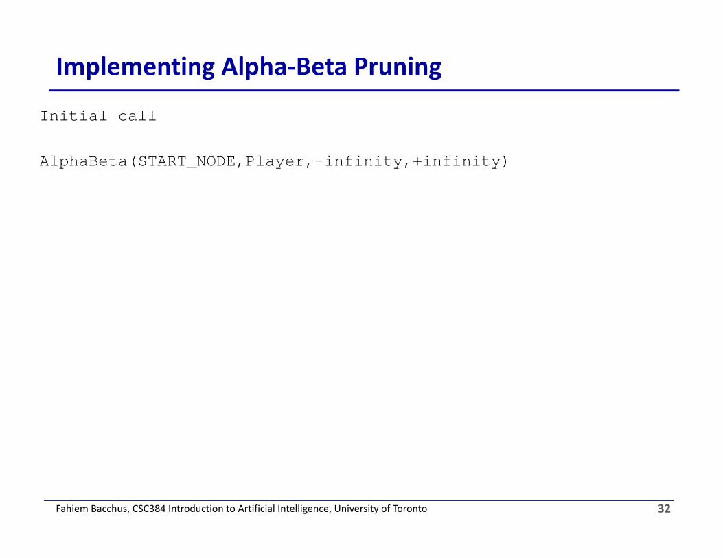
Implementing Alpha‐Beta Pruning

Initial call

AlphaBeta(START_NODE,Player,-infinity,+infinity)


Example

Which computations could we have avoided here? Assuming we expand nodes left to right?

1 Max

Min0 1

1

Max

Min0 2 0 1 -5 2

0 2 1 2

Max

Min

0 3 2 0 1 -5 -3 2

Min0 -3 3 -3 -2 2 -5 0 1 -3 -5 -3 2


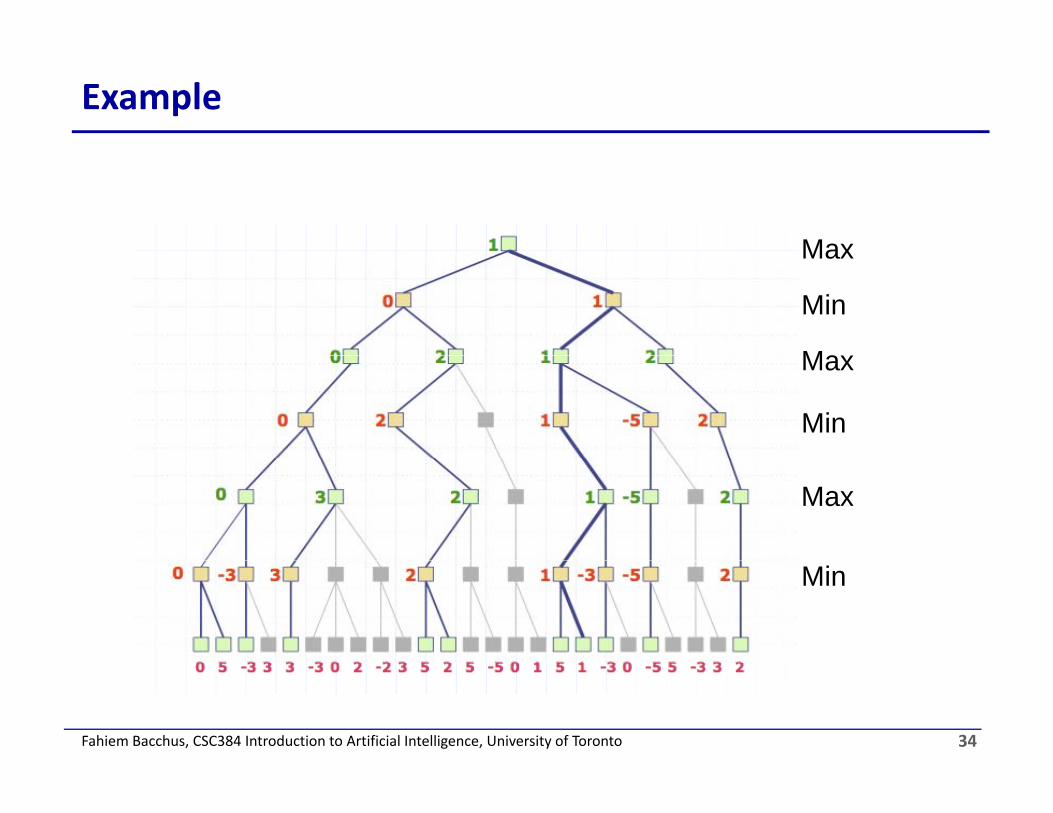
Example

MaxMax

Ma

Min

Max

Min

Max

Min


Effectiveness of Alpha‐Beta Pruning

• With no pruning, you have to explore O(bd) nodes, which makes the run time of a search with pruning the same as plain Minimax.

• If, however, the move ordering for the search is optimal ( i th b t h d fi t) th b f (meaning the best moves are searched first), the number of nodes we need to search using alpha beta pruning is O(bd/2). That means you can, in theory, search twice as d !deep!

• In Deep Blue, they found that alpha beta pruning meant the average branching factor at each node was about 6 average branching factor at each node was about 6 instead of 35.


Rational Opponents

• May want to compute your full strategy ahead of time. • you must store “decisions” for each node you can reach by y y y

playing optimally• if your opponent has unique rational choices, this is a single

branch through game treeg g• if there are “ties”, opponent could choose any one of the “tied”

moves: must store strategy for each subtree• In general space is an issue.In general space is an issue.• Alternatively you compute your next move a fresh at each

stage.


Practical Matters

• All “real” games are too large to enumerate tree• e.g., chess branching factor is roughly 35• Depth 10 tree: 2,700,000,000,000,000 nodes• Even alpha-beta pruning won’t help here!

• We must limit depth of search tree• Can’t expand all the way to terminal nodes• We must make heuristic estimates about the values of the (non-We must make heuristic estimates about the values of the (non

terminal) states at the leaves of the tree• These heuristics are often called evaluation function• evaluation functions are often learnedevaluation functions are often learned


Heuristics in Games

• Example for tic tac toe: h(n) = [# of 3 lengths that are left open for player A] - [# of 3 lengths that are left open for player B].

• Alan Turing’s function for chess: h(n) = A(n)/B(n) where A(n) is the sum of the point value for player A’s pieces and B(n) is the sum for player Bplayer B.

• Most evaluation functions are specified as a weighted sum of features: h(n) = w1*feature1(n) + w2*feature2(n) + ... wi*featurei(n).ea u es: ( ) 1 ea u e1( ) 2 ea u e2( ) ... i ea u ei( ).

• Deep Blue used about 6000 features in its evaluation function.


Heuristics in Games

• Think of a few games and suggest some heuristics for estimating the “goodness” of a positiong g p• Chess?• Checkers?• Your favorite video game?• Your favorite video game?


An Aside on Large Search Problems

• Issue: inability to expand tree to terminal nodes is relevant even in standard search• Often we can’t expect A* to reach a goal by expanding full

frontier• So we often limit our look-ahead, and make moves before we

t ll k th t th t th lactually know the true path to the goal• Sometimes called online or realtime search

• In this case, we use the heuristic function not just to guide our search, but also to commit to moves we actually make• In general, guarantees of optimality are lost, but we reduce

computational/memory expense dramatically


Realtime Search Graphically

1. We run A* (or our favorite search algorithm) until we are forced to make a move or run out until we are forced to make a move or run out of memory. Note: no leaves are goals yet.

2. We use evaluation function f(n) to decide ( )which path looks best (let’s say it is the redone).

fi ( )3. We take the first step along the best path (red), by actually making that move.

4 We restart search at the node we reach by 4. We restart search at the node we reach by making that move. (We may actually cache the results of the relevant part of first search tree if it’s hanging around as it would with A*)


tree if it s hanging around, as it would with A ).

Documents

CSC384: Introduction to Artificial Intelligencefbacchus/csc384/Lectures/csc384-Lecture04-Ga… · CSC384: Introduction to Artificial Intelligence Game Tree Search • Chapter 5.1,