12/4/2016

1

CSC 371- Systems I: Computer

Organization and Architecture

Lecture 13 - Pipeline and Vector

Processing

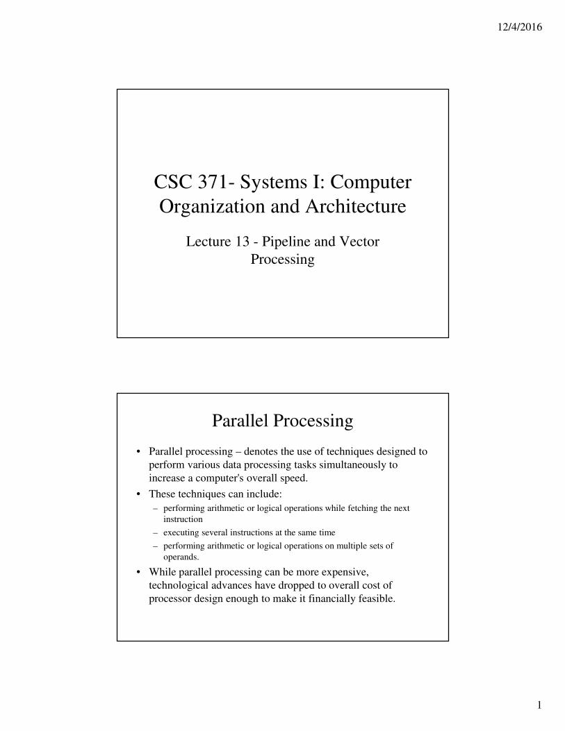
Parallel Processing

• Parallel processing – denotes the use of techniques designed to

perform various data processing tasks simultaneously to

increase a computer's overall speed.

• These techniques can include:

– performing arithmetic or logical operations while fetching the next

instruction

– executing several instructions at the same time

– performing arithmetic or logical operations on multiple sets of

operands.

• While parallel processing can be more expensive,

technological advances have dropped to overall cost of

processor design enough to make it financially feasible.

12/4/2016

2

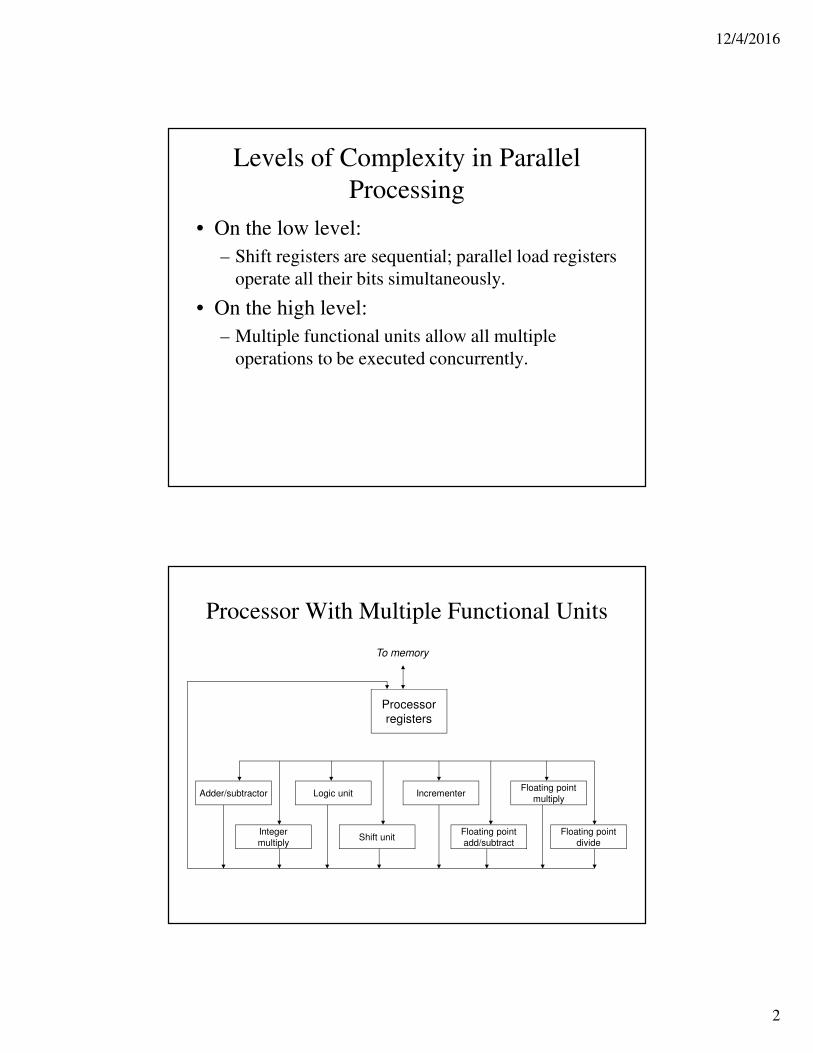
Levels of Complexity in Parallel

Processing

• On the low level:

– Shift registers are sequential; parallel load registers

operate all their bits simultaneously.

• On the high level:

– Multiple functional units allow all multiple

operations to be executed concurrently.

Processor With Multiple Functional Units

Processor

registers

Adder/subtractor

Integer

multiply

Logic unit

Shift unit

Incrementer

Floating point

add/subtract

Floating point

multiply

Floating point

divide

To memory

12/4/2016

3

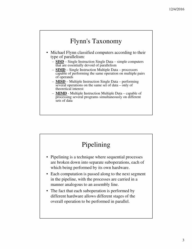
Flynn's Taxonomy

• Michael Flynn classified computers according to their type of parallelism:– SISD – Single Instruction Single Data – simple computers

that are essentially devoid of parallelism

– SIMD – Single Instruction Multiple Data – processors capable of performing the same operation on multiple pairs of operands

– MISD – Multiple Instruction Single Data – performing several operations on the same set of data – only of theoretical interest

– MIMD - Multiple Instruction Multiple Data – capable of processing several programs simultaneously on different sets of data

Pipelining

• Pipelining is a technique where sequential processes

are broken down into separate suboperations, each of

which being performed by its own hardware.

• Each computation is passed along to the next segment

in the pipeline, with the processes are carried in a

manner analogous to an assembly line.

• The fact that each suboperation is performed by

different hardware allows different stages of the

overall operation to be performed in parallel.

12/4/2016

4

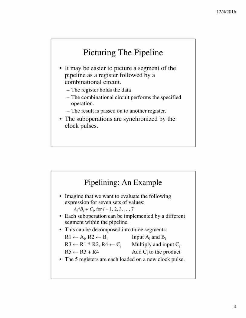
Picturing The Pipeline

• It may be easier to picture a segment of the pipeline as a register followed by a combinational circuit.

– The register holds the data

– The combinational circuit performs the specified operation.

– The result is passed on to another register.

• The suboperations are synchronized by the clock pulses.

Pipelining: An Example

• Imagine that we want to evaluate the following expression for seven sets of values:

Ai*Bi + Ci, for i = 1, 2, 3, …, 7

• Each suboperation can be implemented by a different segment within the pipeline.

• This can be decomposed into three segments:

R1 ← Ai, R2 ← Bi Input Ai and Bi

R3 ← R1 * R2, R4 ← Ci Multiply and input Ci

R5 ← R3 + R4 Add Ci to the product

• The 5 registers are each loaded on a new clock pulse.

12/4/2016

5

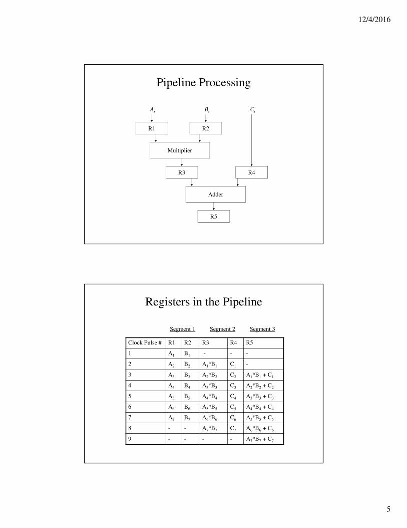
Pipeline Processing

R1 R2

Multiplier

R3 R4

Adder

R5

Ai Bi Ci

Registers in the Pipeline

Clock Pulse # R1 R2 R3 R4 R5

1 A1 B1 - - -

2 A2 B2 A1*B1 C1 -

3 A3 B3 A2*B2 C2 A1*B1 + C1

4 A4 B4 A3*B3 C3 A2*B2 + C2

5 A5 B5 A4*B4 C4 A3*B3 + C3

6 A6 B6 A5*B5 C5 A4*B4 + C4

7 A7 B7 A6*B6 C6 A5*B5 + C5

8 - - A7*B7 C7 A6*B6 + C6

9 - - - - A7*B7 + C7

Segment 2 Segment 3Segment 1

12/4/2016

6

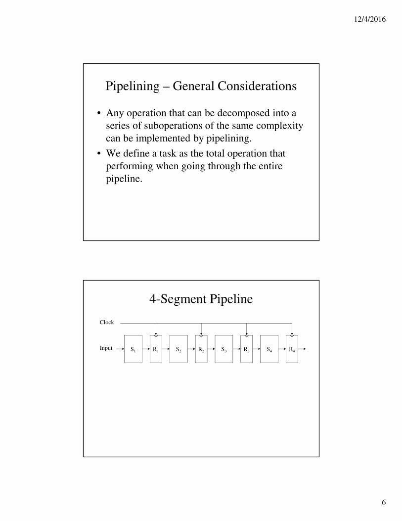
Pipelining – General Considerations

• Any operation that can be decomposed into a

series of suboperations of the same complexity

can be implemented by pipelining.

• We define a task as the total operation that

performing when going through the entire

pipeline.

4-Segment Pipeline

R1S1 R2S2 R3S3 R4S4

Clock

Input

12/4/2016

7

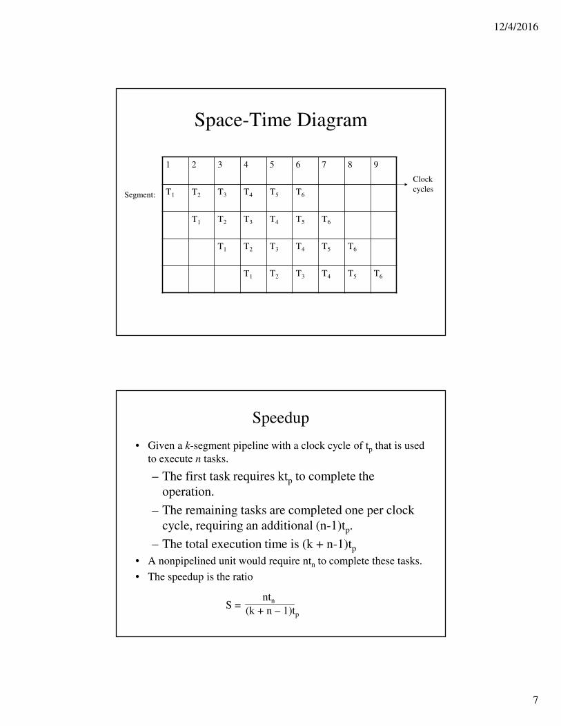
Space-Time Diagram

1 2 3 4 5 6 7 8 9

T1 T2 T3 T4 T5 T6

T1 T2 T3 T4 T5 T6

T1 T2 T3 T4 T5 T6

T1 T2 T3 T4 T5 T6

Segment:

Clock

cycles

Speedup

• Given a k-segment pipeline with a clock cycle of tp that is used

to execute n tasks.

– The first task requires ktp to complete the

operation.

– The remaining tasks are completed one per clock

cycle, requiring an additional (n-1)tp.

– The total execution time is (k + n-1)tp

• A nonpipelined unit would require ntn to complete these tasks.

• The speedup is the ratio

S = ntn

(k + n – 1)tp

12/4/2016

8

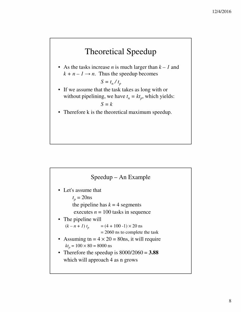
Theoretical Speedup

• As the tasks increase n is much larger than k – 1 and

k + n – 1→ n. Thus the speedup becomes

S = tn / tp

• If we assume that the task takes as long with or

without pipelining, we have tn = ktp, which yields:

S = k

• Therefore k is the theoretical maximum speedup.

Speedup – An Example

• Let's assume that

tp = 20ns

the pipeline has k = 4 segments

executes n = 100 tasks in sequence

• The pipeline will

(k – n + 1) tp = (4 + 100 -1) × 20 ns

= 2060 ns to complete the task

• Assuming tn = 4 × 20 = 80ns, it will require

ktp = 100 × 80 = 8000 ns

• Therefore the speedup is 8000/2060 = 3.88

which will approach 4 as n grows

12/4/2016

9

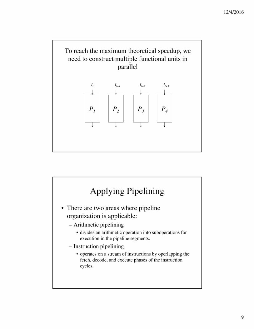
To reach the maximum theoretical speedup, we

need to construct multiple functional units in

parallel

P1

Ii

P2

Ii+1

P3

Ii+2

P4

Ii+3

Applying Pipelining

• There are two areas where pipeline

organization is applicable:

– Arithmetic pipelining

• divides an arithmetic operation into suboperations for

execution in the pipeline segments.

– Instruction pipelining

• operates on a stream of instructions by operlapping the

fetch, decode, and execute phases of the instruction

cycles.

12/4/2016

10

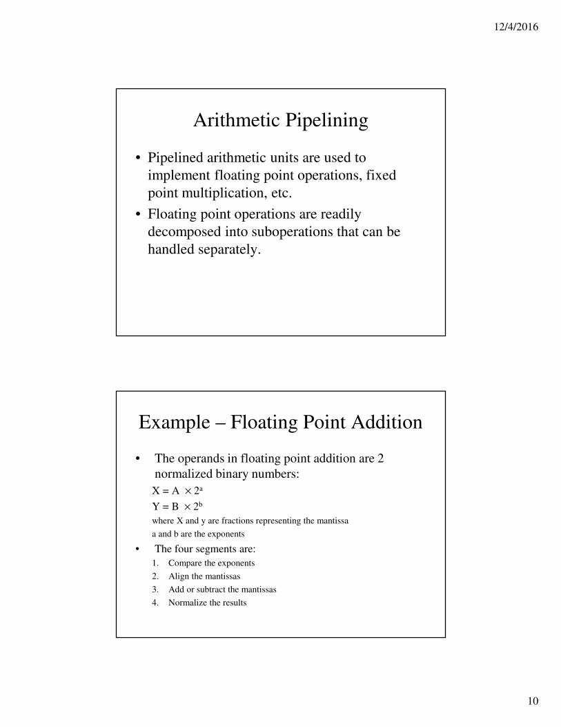
Arithmetic Pipelining

• Pipelined arithmetic units are used to

implement floating point operations, fixed

point multiplication, etc.

• Floating point operations are readily

decomposed into suboperations that can be

handled separately.

Example – Floating Point Addition

• The operands in floating point addition are 2

normalized binary numbers:

X = A × 2a

Y = B × 2b

where X and y are fractions representing the mantissa

a and b are the exponents

• The four segments are:

1. Compare the exponents

2. Align the mantissas

3. Add or subtract the mantissas

4. Normalize the results

12/4/2016

11

Pipeline for Floating Point Addition/SubtractionMantissasExponents

BAa b

R

Compare

exponentsSegment 1:

R

R

Choose

exponent

Align

mantissasSegment 2:

Difference

R

Add/subtract

mantissas

RR

Segment 3:

Normalize

result

R

Adjust

exponent

R

Segment 4:

Example – Floating Point Addition

• If our operands are

X = 0.9504 × 103

Y = 0.8200 × 102

• The difference of the exponents is 3-2 = 1; we adjust Y's exponent:

X = 0.9504 × 103

Y = 0.0820 × 103

• We calculate the product:

Z = 1.0324 × 103

• Then we normalize:

Z = 0.10324 × 104

12/4/2016

12

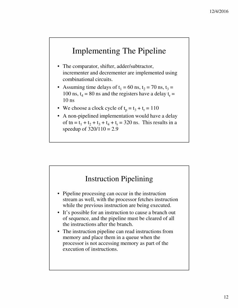
Implementing The Pipeline

• The comparator, shifter, adder/subtractor,

incrementer and decrementer are implemented using

combinational circuits.

• Assuming time delays of t1 = 60 ns, t2 = 70 ns, t3 =

100 ns, t4 = 80 ns and the registers have a delay tr =

10 ns

• We choose a clock cycle of tp = t3 + tr = 110

• A non-pipelined implementation would have a delay

of tn = t1 + t2 + t3 + t4 + tr = 320 ns. This results in a

speedup of 320/110 = 2.9

Instruction Pipelining

• Pipeline processing can occur in the instruction stream as well, with the processor fetches instruction while the previous instruction are being executed.

• It’s possible for an instruction to cause a branch out of sequence, and the pipeline must be cleared of all the instructions after the branch.

• The instruction pipeline can read instructions from memory and place them in a queue when the processor is not accessing memory as part of the execution of instructions.

12/4/2016

13

Steps in the Instruction Cycle

• Computers with complex instructions require several phases in order to process an instruction. These might include:

1. Fetch the instruction from memory

2. Decode the instruction

3. Calculate the effective address

4. Fetch the operands from memory

5. Execute the instruction

6. Store the result in the proper place

Difficulties Slowing Down the

Instruction Pipeline

• Certain difficulties can prevent the instruction

pipeline from operating at maximum speed:

– Different segments may require different amounts of time

(pipelining is most efficient with segments of the same

duration)

– Some segments are skipped for certain operations (e.g.,

memory reads for register-reference instructions)

– More that one segment may require memory access at the

same time (this can be resolve with multiple busses).

12/4/2016

14

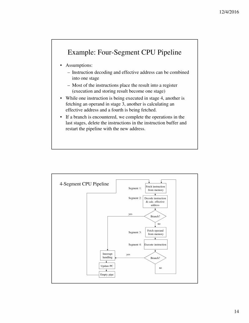
Example: Four-Segment CPU Pipeline

• Assumptions:

– Instruction decoding and effective address can be combined

into one stage

– Most of the instructions place the result into a register

(execution and storing result become one stage)

• While one instruction is being executed in stage 4, another is

fetching an operand in stage 3, another is calculating an

effective address and a fourth is being fetched.

• If a branch is encountered, we complete the operations in the

last stages, delete the instructions in the instruction buffer and

restart the pipeline with the new address.

4-Segment CPU PipelineFetch instruction

from memory

Decode instruction

& calc. effective

address

Segment 1:

Segment 2:

Branch?

Fetch operand

from memorySegment 3:

no

Execute instruction Segment 4:

Branch?

Interrupt

handling

no

yes

Update PC

Empty pipe

yes

12/4/2016

15

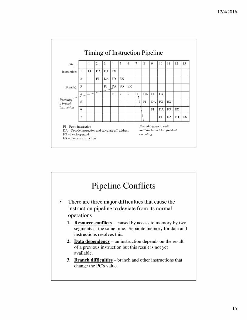
Timing of Instruction Pipeline

1 2 3 4 5 6 7 8 9 10 11 12 13

1 FI DA FO EX

2 FI DA FO EX

3 FI DA FO EX

4 FI - - FI DA FO EX

5 - - - FI DA FO EX

6 FI DA FO EX

7 FI DA FO EX

Step:

Instruction:

(Branch)

FI – Fetch instruction

DA – Decode instruction and calculate eff. address

FO – Fetch operand

EX – Execute instruction

Decoding

a branch

instruction

Everything has to wait

until the branch has finished

executing

Pipeline Conflicts

• There are three major difficulties that cause the

instruction pipeline to deviate from its normal

operations

1. Resource conflicts – caused by access to memory by two

segments at the same time. Separate memory for data and

instructions resolves this.

2. Data dependency – an instruction depends on the result

of a previous instruction but this result is not yet

available.

3. Branch difficulties – branch and other instructions that

change the PC's value.

12/4/2016

16

Data Dependency

• A data dependency occurs when an instruction needs data that is not yet available.

• An instruction may need to fetch an operand being generated at the same time by an instruction that is first being executed.

• An address dependency occurs when an address cannot be calculated because the necessary information is not yet available, e.g., an instruction with an register indirect address cannot fetch the operand because the address is not yet loaded into the register.

Dealing With Data Dependency

• Pipelined computers deal with data dependencies in several ways:

– Hardware interlocks - a circuit that detects instructions whose source operands are destinations of instructions farther up in the pipeline. It delays the later instructions.

– Operand forwarding – if a result is needed as a source in an instruction that is further down the pipeline, it is forwarded there, bypassing the register file. This requires special circuitry.

– Delayed load – using a compiler that detects data dependencies in programs and adds NOP instructions to delay the loading of the conflicted data.

12/4/2016

17

Handling Branch Instructions

• Branch instructions are a major problem in operating an instruction pipeline, whether they are unconditional (always occur) or conditional(depending on whether the condition is satisfied).

• These can be handled by several approaches:

– Prefetching target instruction – Both the target instruction (of the branch) and the next instruction are fetched and saved until the branch is executed. This can be extended to include instructions after both places in memory.

– Use of a branch target buffer – the target address and the instruction at that address are both stored in associative memory (along with the next few instructions).

Handling Branch Instructions (continued)

– Using a loop buffer – a small high-speed register file that

stores the instructions of a program loop when it is

detected.

– Branch prediction – guesses the outcome of a condition

and prefetches instructions

– Delayed branch – used by most RISC processors. Branch

instructions are detected and object code is rearranged by

inserting instructions that keep the pipeline going. (This

can be NOPs).

12/4/2016

18

RISC Pipeline

• The RISC architecture is able to use an efficient pipeline that uses a small number of suboperations for several reasons:

– Its fixed length format means that decoding can occur during register selection

– Data manipulation are all done using register-to-register operations, so there is no need to calculate effective addresses.

– This means that instructions can be carried out in 3 subsoperations, with the third used for storing the result in the specified register.

RISC Architecture and Memory-

Reference Instructions

• The only data transfer instructions in RISC architecture are load and store, which use register indirect addressing, which typically requires 3-4 stages in the pipeline.

• Conflicts between instruction fetches and transferring the operand can be avoid with multiple busses that access separate memories for data and instructions.

12/4/2016

19

Advantages of RISC Architecture

• RISC processors are able to execute

instructions at a rate of one instruction per

clock cycle.

– Each instruction can be started with a new clock

cycle and the processor is pipelined so the one

clock cycle per instruction rate can be achieved.

• RISC processors can rely on the compiler to

detect and minimize the delays caused by data

conflicts and branch penalties.

Example: 3-Segment Instruction

Pipeline

• A typical RISC processor will have 3

instruction formats:

– Data manipulation instructions use registers only

– Data transfer instructions use an effective address

consisting of register contents and constant offset

– Program control instructions use registers and a

constant to evaluate the branch address.

12/4/2016

20

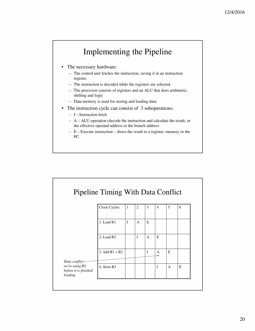
Implementing the Pipeline

• The necessary hardware:

– The control unit fetches the instruction, saving it in an instruction

register.

– The instruction is decoded while the registers are selected.

– The processor consists of registers and an ALU that does arithmetic,

shifting and logic

– Data memory is used for storing and loading data.

• The instruction cycle can consist of 3 suboperations:

– I – Instruction fetch

– A – ALU operation (decode the instruction and calculate the result, or

the effective operand address or the branch address

– E – Execute instruction – direct the result to a register, memory or the

PC

Pipeline Timing With Data Conflict

Clock Cycles: 1 2 3 4 5 6

1. Load R1 I A E

2. Load R2 I A E

3. Add R1 + R2 I A E

4. Store R3 I A E

Data conflict

we're using R2

before it is finished

loading

12/4/2016

21

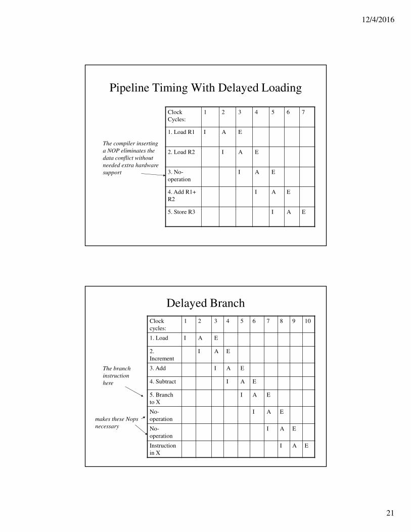
Pipeline Timing With Delayed Loading

Clock

Cycles:

1 2 3 4 5 6 7

1. Load R1 I A E

2. Load R2 I A E

3. No-

operation

I A E

4. Add R1+

R2

I A E

5. Store R3 I A E

The compiler inserting

a NOP eliminates the

data conflict without

needed extra hardware

support

Delayed Branch

Clock

cycles:

1 2 3 4 5 6 7 8 9 10

1. Load I A E

2.

Increment

I A E

3. Add I A E

4. Subtract I A E

5. Branch

to X

I A E

No-

operation

I A E

No-

operation

I A E

Instruction

in X

I A E

The branch

instruction

here

makes these Nops

necessary

12/4/2016

22

Delayed Branch

Clock

cycles:

1 2 3 4 5 6 7 8 9 10

1. Load I A E

2.

Increment

I A E

3. Branch

to X

I A E

4. Add I A E

5. Subtract I A E

Instruction

in X

I A E

Placing the

branch

instruction

here

makes a Nop

instruction

here

unecessary

Vector Processing

• There is a class of computation problems that require far greater computation power than many computers can provide. They can take days or weeks to solve on conventional computers.

• These problems can be formulated in terms of vectors and matrices.

• Computers that can process vectors as a unit can solve these problems much more easily.

12/4/2016

23

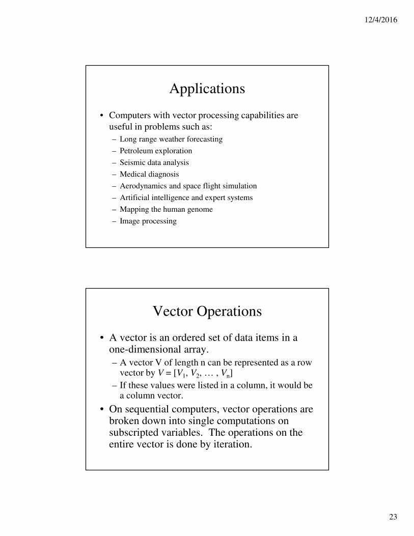
Applications

• Computers with vector processing capabilities are

useful in problems such as:

– Long range weather forecasting

– Petroleum exploration

– Seismic data analysis

– Medical diagnosis

– Aerodynamics and space flight simulation

– Artificial intelligence and expert systems

– Mapping the human genome

– Image processing

Vector Operations

• A vector is an ordered set of data items in a one-dimensional array.

– A vector V of length n can be represented as a row vector by V = [V1, V2, … , Vn]

– If these values were listed in a column, it would be a column vector.

• On sequential computers, vector operations are broken down into single computations on subscripted variables. The operations on the entire vector is done by iteration.

12/4/2016

24

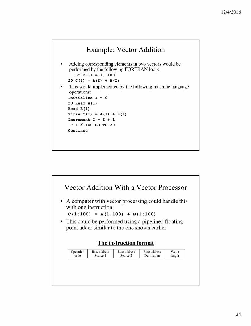
Example: Vector Addition

• Adding corresponding elements in two vectors would be performed by the following FORTRAN loop:

DO 20 I = 1, 100

20 C(I) = A(I) + B(I)

• This would implemented by the following machine language operations:Initialize I = 0

20 Read A(I)

Read B(I)

Store C(I) = A(I) + B(I)

Increment I = I + 1

IF I ≤ 100 GO TO 20

Continue

Vector Addition With a Vector Processor

• A computer with vector processing could handle this with one instruction:C(1:100) = A(1:100) + B(1:100)

• This could be performed using a pipelined floating-point adder similar to the one shown earlier.

The instruction format

Operation

code

Base address

Source 1

Base address

Source 2

Base address

Destination

Vector

length

12/4/2016

25

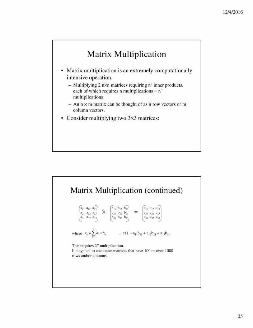
Matrix Multiplication

• Matrix multiplication is an extremely computationally

intensive operation.

– Multiplying 2 n×n matrices requiring n2 inner products,

each of which requires n multiplications = n3

multiplications

– An n × m matrix can be thought of as n row vectors or m

column vectors.

• Consider multiplying two 3×3 matrices:

Matrix Multiplication (continued)

a11 a12 a13

a21 a22 a23

a31 a32 a33

b11 b12 b13

b21 b22 b23

b31 b32 b33

c11 c12 c13

c21 c22 c23

c31 c32 c33

× =

where kj

k

ikij bac ×=∑=

3

1

∴ c11 = a11b11 + a12b21 + a13b31

This requires 27 multiplication.

It is typical to encounter matrices that have 100 or even 1000

rows and/or columns.

12/4/2016

26

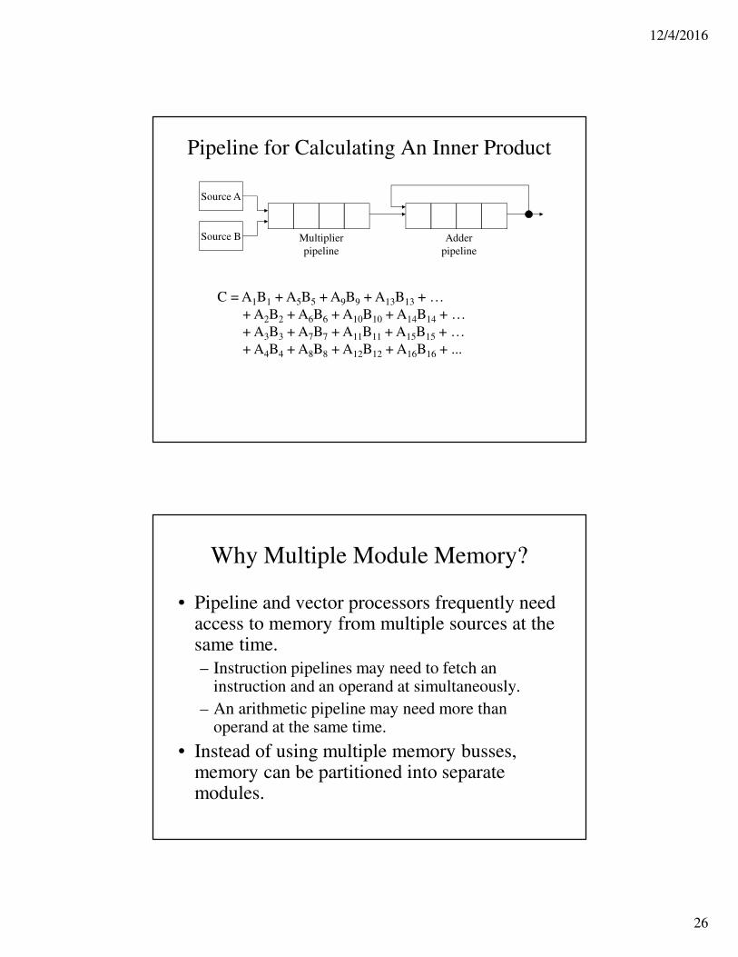
Pipeline for Calculating An Inner Product

Source A

Source B Multiplier

pipeline

Adder

pipeline

C = A1B1 + A5B5 + A9B9 + A13B13 + …

+ A2B2 + A6B6 + A10B10 + A14B14 + …

+ A3B3 + A7B7 + A11B11 + A15B15 + …

+ A4B4 + A8B8 + A12B12 + A16B16 + ...

Why Multiple Module Memory?

• Pipeline and vector processors frequently need access to memory from multiple sources at the same time.

– Instruction pipelines may need to fetch an instruction and an operand at simultaneously.

– An arithmetic pipeline may need more than operand at the same time.

• Instead of using multiple memory busses, memory can be partitioned into separate modules.

12/4/2016

27

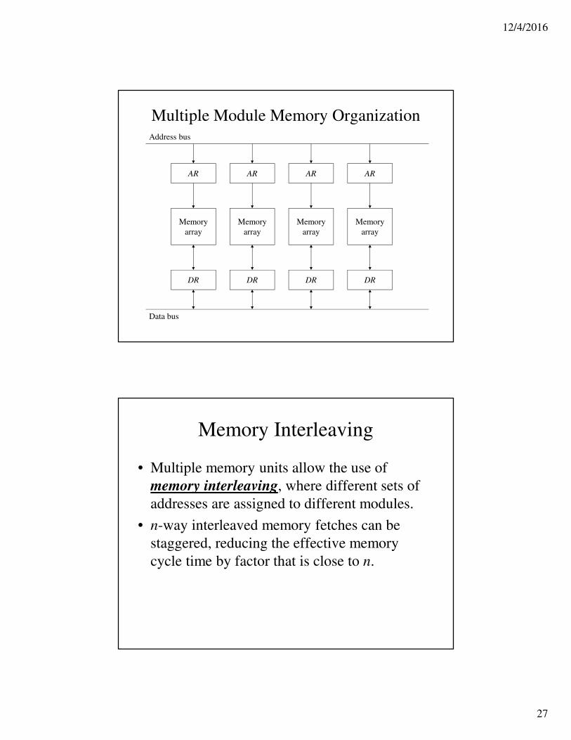
Multiple Module Memory Organization

Memory

array

Memory

array

Memory

array

Memory

array

AR AR AR AR

DR DR DR DR

Address bus

Data bus

Memory Interleaving

• Multiple memory units allow the use of

memory interleaving, where different sets of

addresses are assigned to different modules.

• n-way interleaved memory fetches can be

staggered, reducing the effective memory

cycle time by factor that is close to n.

12/4/2016

28

Supercomputers

• Supercomputers are commercial computers with vector

instructions and pipeline floating-point arithmetic operations.

– Components are also placed in close proximity to speed

data transfers and require special cooling because of the

resultant heat build-up.

• Supercomputers have all the standard instructions that one

might expect as well as those for vector operations. They have

multiple functional units, each with their own pipeline.

• They also make heavy use of parallel processing and are

optimized for large-scale numerical operations.

Supercomputers and Performance

• Supercomputer performance are usually

measured in terms of floating-point operations

per second (flops). Derivative terms include

megaflops and gigaflops.

• Typical supercomputer has a cycle time of 4

to 20 ns.

– With one floating-point operation per cycle, this

can lead to performance of 50 to 250 megaflops.

(This does not include set-up time).

12/4/2016

29

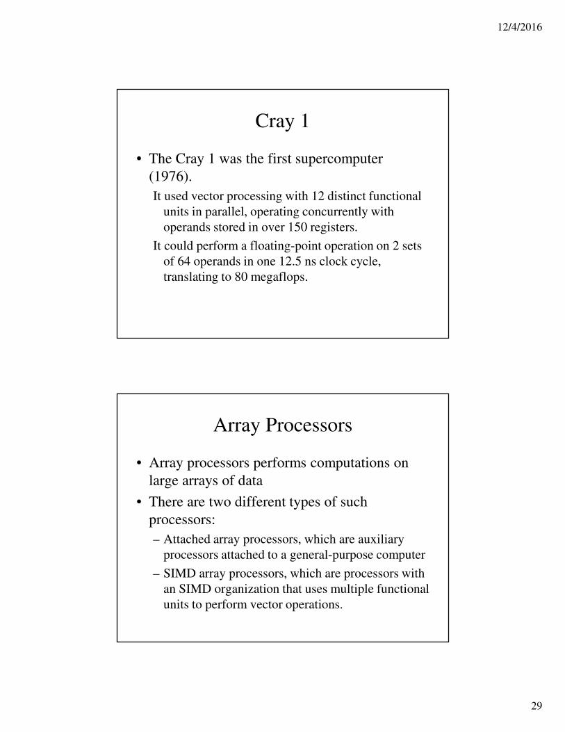
Cray 1

• The Cray 1 was the first supercomputer

(1976).

It used vector processing with 12 distinct functional

units in parallel, operating concurrently with

operands stored in over 150 registers.

It could perform a floating-point operation on 2 sets

of 64 operands in one 12.5 ns clock cycle,

translating to 80 megaflops.

Array Processors

• Array processors performs computations on

large arrays of data

• There are two different types of such

processors:

– Attached array processors, which are auxiliary

processors attached to a general-purpose computer

– SIMD array processors, which are processors with

an SIMD organization that uses multiple functional

units to perform vector operations.

12/4/2016

30

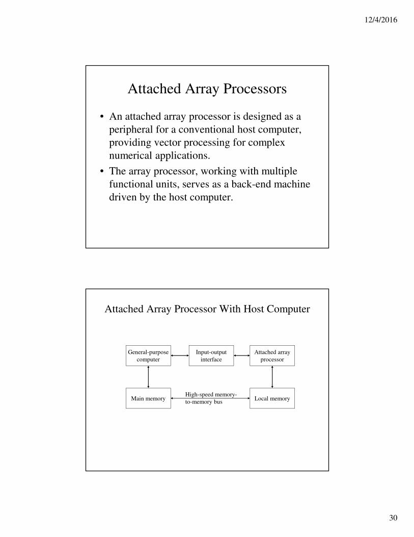
Attached Array Processors

• An attached array processor is designed as a

peripheral for a conventional host computer,

providing vector processing for complex

numerical applications.

• The array processor, working with multiple

functional units, serves as a back-end machine

driven by the host computer.

Attached Array Processor With Host Computer

General-purpose

computer

Input-output

interface

Attached array

processor

Main memory Local memoryHigh-speed memory-

to-memory bus

12/4/2016

31

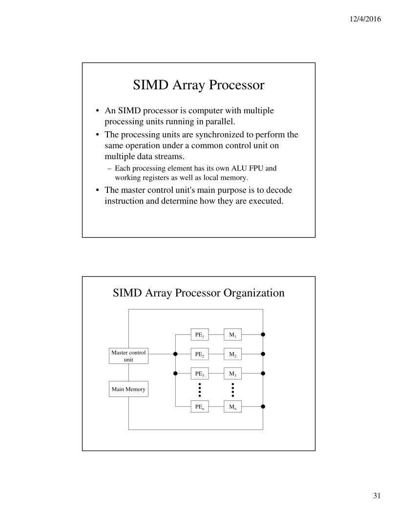
SIMD Array Processor

• An SIMD processor is computer with multiple

processing units running in parallel.

• The processing units are synchronized to perform the

same operation under a common control unit on

multiple data streams.

– Each processing element has its own ALU FPU and

working registers as well as local memory.

• The master control unit's main purpose is to decode

instruction and determine how they are executed.

SIMD Array Processor Organization

Master control

unit

Main Memory

PE1

PE2

PE3

PEn

M1

M2

M3

Mn