Embed Size (px)
Citation preview
VELTECH HIGHTECH Dr.RANGARAJAN Dr.SAKUNTHALA ENGINEERING COLLEGE DEPARTMENT OF COMPUTER SCIENCE AND ENGINEERING
VELTECH Dr.RANGARAJAN Dr.SAKUNTHALA ENGINEERING COLLEGE Page 1
CS6704_RESOURCES MANAGEMENT TECHNIQUES
UNIT I
Resources management techniques or Operations Research deals with different
techniques for optimal use of resources and to ultimately optimize the Objective
function.
The natural resources available are limited except the air. The question how
judiciously they have to be utilized to maximize the Objective function. Since
RMT is mostly applied to Business the Objectives are maximization of Profit,
Income and minimization of Loss, expenditure. Etc.
RMT is applied in department as:
1. Allocation and Distribution
2. Production and Facility Planning
3. Procurement
4. Marketing
5. Finance
6. Personnel and
7. Research and Development.
One of the definitions of OR or RMT RUNS AS FOLLOWS
It is aid for the Executive in making his decisions by providing him with the
needed quantitative information based on the scientific method of analysis.
This was given by C.Kittel.
RMT is the science of efficient way of managing the resources for optimization
of objectives against certain constraints. By resource me mean some of them
like man, machine, money, land, time, raw materials and other resources.
Therefore Decision making is very important skill a person must possess to be
successful. Thus it is a decision science that helps a management to make
better decisions.
VELTECH HIGHTECH Dr.RANGARAJAN Dr.SAKUNTHALA ENGINEERING COLLEGE DEPARTMENT OF COMPUTER SCIENCE AND ENGINEERING
VELTECH Dr.RANGARAJAN Dr.SAKUNTHALA ENGINEERING COLLEGE Page 2
The essential characteristics of decision making are
1. Objectives
2. Alternatives
3. Influencing factors( constraints)
Phases of RMT
1 Formulating the problem
2 Constructing the model to represent the system under study
3 Deriving solution from the model
4 Testing the model with obtained solution.
5 Establishing control over the solution
6 Implementation.
CONSTRUCTION OF MODEL is an important phase of the RMT to optimize the
objective function.
Definition of a model:
A model is a reasonably simplified representation of a real world situation. It is an
abstraction of reality.
Models can be classified as
(i) Iconic models
(ii) Analogue models
(iii) Deterministic models
(iv) Stochastic models.
1. Iconic models: This is a physical or pictorial representation of various aspects
of a system.

VELTECH HIGHTECH Dr.RANGARAJAN Dr.SAKUNTHALA ENGINEERING COLLEGE DEPARTMENT OF COMPUTER SCIENCE AND ENGINEERING
VELTECH Dr.RANGARAJAN Dr.SAKUNTHALA ENGINEERING COLLEGE Page 3
e.g. Toy, miniature model of a building, the bar graph of a company, etc.
2. Analogue models: This uses one set of properties to represent another set of
properties which a system under study has.
e.g. A network of water pipes to represent the flow of current in an electrical net
work or graphs , organizational charts ,etc.
3. Mathematical symbolic model: This uses a set of mathematical symbols ( letter,
numbers, etc) to represent the decision variables of a system under
consideration. These variables are related by mathematical equations or in
equations which describe the property of the system.
e.g A linear Programming Problem (LPP), Non linear Programming problem, etc.
4. Static model: This is a model which does not take account time as a
parameter. It assumes that the value of the variables do not change with time
during a period of time horizon.
e.g. LPP. Assignment problem, Transportation problem. Etc.
5. Dynamic model: Here time is considered as one of the important variables.
e.g. Dynamic Programming Problem , Replacement Problem, etc.
6 Deterministic model: Here uncertainty is not taken into account,
e.g. LPP. AP. TP. Etc.
7. Stochastic models: This considers uncertainty as important aspect of the
problem
e.g. Queuing models, inventory of stochastic nature, etc.
CHARACTERISTIC of a good model:
1 Must be simple
2. Must be designed to accept any changes.
VELTECH HIGHTECH Dr.RANGARAJAN Dr.SAKUNTHALA ENGINEERING COLLEGE DEPARTMENT OF COMPUTER SCIENCE AND ENGINEERING
VELTECH Dr.RANGARAJAN Dr.SAKUNTHALA ENGINEERING COLLEGE Page 4
3. Assumptions must be as small as possible.
4. Number of variables must be small.
5. Must be open to parametric treatment.
Principles pf modeling:
1. Do not build complicated models.
2. Beware of moulding the problems to fit a technique.
3. Careful deductions are necessary.
4. Validated prior to implementation
5. Solution can’t be accurate unless variables are properly chosen.
6. Must act as Aid for decision making.
7. Must be as accurate as possible.
The various methods of solving a model are :
1. Analytic method
2. Iterative method
3. Monte-Carlo technique.
The main Phases of RMT are:
1. Formulation of the problem
2. Construction of mathematical model
3. Solving the constructed model
4. Controlling and updating
5. Testing the model and its solution.
6. Implementation.
LIMITATION of RMT:
RMT does not take into account quantitative or emotional or some human
factors which are essential for decision making.
FORMULATION OF LPP:
VELTECH HIGHTECH Dr.RANGARAJAN Dr.SAKUNTHALA ENGINEERING COLLEGE DEPARTMENT OF COMPUTER SCIENCE AND ENGINEERING
VELTECH Dr.RANGARAJAN Dr.SAKUNTHALA ENGINEERING COLLEGE Page 5
Given a problem, identify the objective function, the decision variables and the
constraints, the mathematical formulation is :
Optimize Z = f( x1 , x2, x3, ……….. xn)
Subject to constraints:
gj(x1 , x2, x3, ……….. xn ) ≤ = ≥ bj j= 1,2, ………………m.
xi ≥ 0 for all i = 1,2,……………n
Z is the objective function, it depends on the decision variables xi ≥ 0 for all I =
1,2,……………n for its optimization
gj(x1 , x2, x3, ……….. xn ) ≤ = ≥ bj are the m constraints of the LPP.
Note that , here f( x1 , x2, x3, ……….. xn) = c1x1 + c2x2 +…………+ cnxn
c1, c2,…………,cn are assumed to be known in advance.
b1, b2,…………,bn the constants on the rhs of the constraints are assumed to be
known ( availability)
The coefficient matrix A = (ai j ), which are the coefficients of the decision
variables in the constraints are assumed to be known.
[In ordinary course the above need not be true ]
The mathematical formulation can also be given as :
Optimize z = c1x1 + c2x2 +…………+ cnxn
Subject to constraints:
a11x1 + a12x2 +…………+ a1nxn ≤ = ≥ b1
a21x1 + a22x2 +…………+ a2nxn ≤ = ≥ b2
a31x1 + a32x2 +…………+ a3nxn ≤ = ≥ b3 (I)
………………………………………………………..
VELTECH HIGHTECH Dr.RANGARAJAN Dr.SAKUNTHALA ENGINEERING COLLEGE DEPARTMENT OF COMPUTER SCIENCE AND ENGINEERING
VELTECH Dr.RANGARAJAN Dr.SAKUNTHALA ENGINEERING COLLEGE Page 6
…………………………………………………………
Am1x1 + am2x2 +…………+ amnxn ≤ = ≥ bm
xi ≥ 0 for all i = 1,2,……………n which cal also be written as
Optimise Z = CX subject
AX = b and X ≥ 0 where C , b are as explained and the A is the matrix of the
coefficients of the decision variables in the constraints.
1. Solution of an LPP: By solution of an LPP we mean finding the values of the
decision variables which satisfy all the constraints given in the LPP.
2. Feasible solution: A solution of an LPP is said to be feasible if they satisfy
the non negative constraints i.e all the decision variables must greater than
or zero.
3. Optimal solution: By optimal solution of an LPP we mean the feasible
solution of the LPP optimizing the objective function.
An LPP of the form (I) is said to be in CANNONICAL form if optimization is
MAXIMIZATION and all the constraints are LESS THAN OR EQUAL TO .
An LPP of the form (I) is said to be in STANDARD form if optimization is
MAXIMIZATION and all the constraints are EQUAL TO. The decision variables
are non negative.
The solution to an LPP with two decision variables can be solved by graphical
method.
1. We draw the equations of the constraints and they are straight lines.
2. Keeping these as reference lines identify the regions the in equations
define, whether above the line or below the line and mark it with a shade.
3. Every constraint will define a region that they may all bound a common
region , which contains all those points that satisfy all the constraints given
in the problem. We call this region as FEASIBLE REGION.
VELTECH HIGHTECH Dr.RANGARAJAN Dr.SAKUNTHALA ENGINEERING COLLEGE DEPARTMENT OF COMPUTER SCIENCE AND ENGINEERING
VELTECH Dr.RANGARAJAN Dr.SAKUNTHALA ENGINEERING COLLEGE Page 7
4. Therefore a feasible region is one , bounded by all the lines of constraints
and contains all those points that satisfy all the constraints given in the
problem.
5. Optimal value of objective function occurs at the vertices of the
polyhydron formed by the lines.
6. For maximisation problem the optimal vertex ( vertices) will be away from
the origin whereas for a minimisation problem the vertex(vertices) will be
closer to the origin.
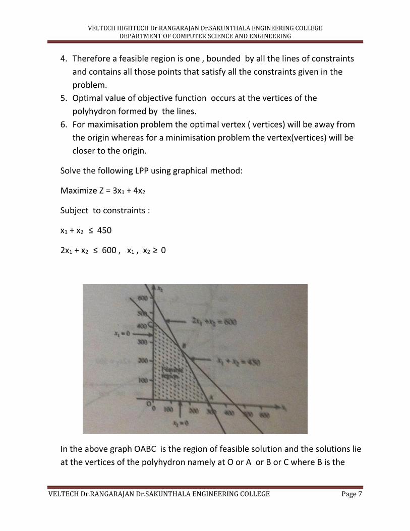
Solve the following LPP using graphical method:
Maximize Z = 3x1 + 4x2
Subject to constraints :
x1 + x2 ≤ 450
2x1 + x2 ≤ 600 , x1 , x2 ≥ 0
In the above graph OABC is the region of feasible solution and the solutions lie
at the vertices of the polyhydron namely at O or A or B or C where B is the
VELTECH HIGHTECH Dr.RANGARAJAN Dr.SAKUNTHALA ENGINEERING COLLEGE DEPARTMENT OF COMPUTER SCIENCE AND ENGINEERING
VELTECH Dr.RANGARAJAN Dr.SAKUNTHALA ENGINEERING COLLEGE Page 8
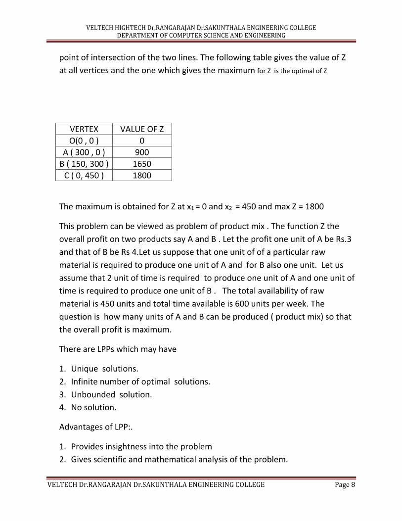
point of intersection of the two lines. The following table gives the value of Z
at all vertices and the one which gives the maximum for Z is the optimal of Z
VERTEX VALUE OF Z
O(0 , 0 ) 0
A ( 300 , 0 ) 900 B ( 150, 300 ) 1650
C ( 0, 450 ) 1800
The maximum is obtained for Z at x1 = 0 and x2 = 450 and max Z = 1800
This problem can be viewed as problem of product mix . The function Z the
overall profit on two products say A and B . Let the profit one unit of A be Rs.3
and that of B be Rs 4.Let us suppose that one unit of of a particular raw
material is required to produce one unit of A and for B also one unit. Let us
assume that 2 unit of time is required to produce one unit of A and one unit of
time is required to produce one unit of B . The total availability of raw
material is 450 units and total time available is 600 units per week. The
question is how many units of A and B can be produced ( product mix) so that
the overall profit is maximum.
There are LPPs which may have
1. Unique solutions.
2. Infinite number of optimal solutions.
3. Unbounded solution.
4. No solution.
Advantages of LPP:.
1. Provides insightness into the problem
2. Gives scientific and mathematical analysis of the problem.
VELTECH HIGHTECH Dr.RANGARAJAN Dr.SAKUNTHALA ENGINEERING COLLEGE DEPARTMENT OF COMPUTER SCIENCE AND ENGINEERING
VELTECH Dr.RANGARAJAN Dr.SAKUNTHALA ENGINEERING COLLEGE Page 9
3. Deals with changing situations.
4. Gives the best solution possible
Limitation of LPP:
1. Assumption of linear relationship only.
2. All parameters assumed to be known.
3. More number of variables and constraints make more complicated and
difficult to solve.
4. Always deals with one objective only.
Note that a feasible region is a convex region. A convex region is one in which
the join any two random points lie in the same region.
The basic assumptions made in Lapp are :
1. Proportionality: When the proportion of input increases the out put will
also increase in the corresponding proportion.
2. Divisibility: The values of decision variables can be non integers.
3. Coefficients of decision variables in objective function and in constraints
are assumed to be known.
4. The availability of resources are assumed to be known.
5. Variables and constraints are finite in number.
6. Optimality. Objective function is optimised.
SLACK Variable.
∑ 𝑎𝑖𝑗𝑛𝑗=1 𝑥𝑖𝑗 ≤ bi i = 1, 2, ……….k
∑ 𝑎𝑖𝑗𝑛𝑗=1 𝑥𝑖𝑗 + si = bi i = 1, 2, ……….k
si ≥ 0 called slack variable and it signifies unused resources.
SURPLUS Variable:
∑ 𝑎𝑖𝑗𝑛𝑗=1 𝑥𝑖𝑗 ≥ bi i = k, k+1,………..
The above can be written as ∑ 𝑎𝑖𝑗𝑛𝑗=1 𝑥𝑖𝑗 - si = bi , i = k, k+1,………..
VELTECH HIGHTECH Dr.RANGARAJAN Dr.SAKUNTHALA ENGINEERING COLLEGE DEPARTMENT OF COMPUTER SCIENCE AND ENGINEERING
VELTECH Dr.RANGARAJAN Dr.SAKUNTHALA ENGINEERING COLLEGE Page 10
Here si ≥ 0 is called surplus variable and signifies excess used resource.
Unrestricted variable:
Avariable x is said to be unrestricted variable if it can be expressed as
x = x ’ + x” and x ’, x” ≥ 0
Simple method:
This is also called iteration method, this method is applied when the number
of constraints are large or the number of decision variables are more than two.
In this method we first find the initial solution called basic solution and using
iterative method improve the solution under certain optimality conditions.
Certain Definitions:
1. Basic solution: If there are n variables and m equations ( n > m ), n – m
variables are made as zeros and they are called as non basic variables and
the m variables are called basic variables and is called the basis of the
problem.
2. Non degenerate basic solution: It is a basic solution if none of the basic
variables are zero.
3. Degenerate basic solution: It is a basic solution in which one or more basic
variable are zero.
4. Basic feasible solution: A feasible solution which is also basic is called basic
feasible solution.
Note
1. we use simplex method to solve Maximization of LPP, Minimization is
solved by converting the minimization to maximization problem as:
This method is also called iteration method. A basic solution is found and Is
improved by the process of iteration under the condition of optimality. A
solution is said to be obtained for the LPP if optimality condition is satisfied
or that it becomes certain that no solution exists for the problem.
VELTECH HIGHTECH Dr.RANGARAJAN Dr.SAKUNTHALA ENGINEERING COLLEGE DEPARTMENT OF COMPUTER SCIENCE AND ENGINEERING
VELTECH Dr.RANGARAJAN Dr.SAKUNTHALA ENGINEERING COLLEGE Page 11
Simplex method is employed when the number of constraints or there are
more than two variables in the LPP.
Min Z = - Max( -Z) = - Max ( Z*) where Z* = -Z. Now we solve for Max Z* and
after solving and finding the optimal solution , we get the solution to the
original problem by “ – MaxZ* = - Max ( -Z ) for the same values of decision
variables.[ Z* = -f(x) ]
2. When constraints are ≥ or = , then the initial solution that is the basic
solution will be negative. Normally the basic solution should never be negative
( if so solved by dual simplex method ) , to overcome situations of that type we
introduce Artificial variables and use them to solve the problem but they form
a part of the solution.
Procedure to solve using simplex method.:
Given an LPP, in cannonical form convert into standard form , if minisation
convert to maximization.
Make n – m variables as zeros and with m basic variables for the iteration to
improve the basic solutions. Solution is optimized with an optimality condition.
The iterations are carried out till the optimality condition is satisfied. By when
we would have arrived at the solution or confirmed that solution does not
exist.
In the case of Big M method or Big M technique or Charnes method to get rid
of artificial variables we assign a very big penalty ( –M for maximization and
+M for minimization problems.)as the coefficients of artificial variables in the
objective function.
While solving note the following:
1. If no artificial variables remain in the basis ( under XB ) and optimality
condition is satisfied , then we have got optimal basic feasible solution.
VELTECH HIGHTECH Dr.RANGARAJAN Dr.SAKUNTHALA ENGINEERING COLLEGE DEPARTMENT OF COMPUTER SCIENCE AND ENGINEERING
VELTECH Dr.RANGARAJAN Dr.SAKUNTHALA ENGINEERING COLLEGE Page 12
2. If atleast one artificial variable remains in the basis in zero level and
optimality condition is satisfied , then current solution is an optimal basic
feasible solution though it is degenerated.
3. If atleast one artificial variable remains in the basis in non zero level and
optimality condition is satisfied , then the original problem does not have
feasible solution. The solution satisfies the constraints but does not
optimise the objective function as it contains a very large M and is called
Pseudo- optimal solutiois an optimal basic feasible solution though it is
degenerated.
Example: Solve the following Lpp using simplex method:
Max z = 5X1 + 12X2 + 8X3
subject to:
3X1 + 4X2 + 5X3 ≤ 60
5X1 + 4X2 + 4X3 ≤ 72
2X1 + 4X2 + 5X3 ≤ 100, X1 ,X2 ,X3 ≥ 0
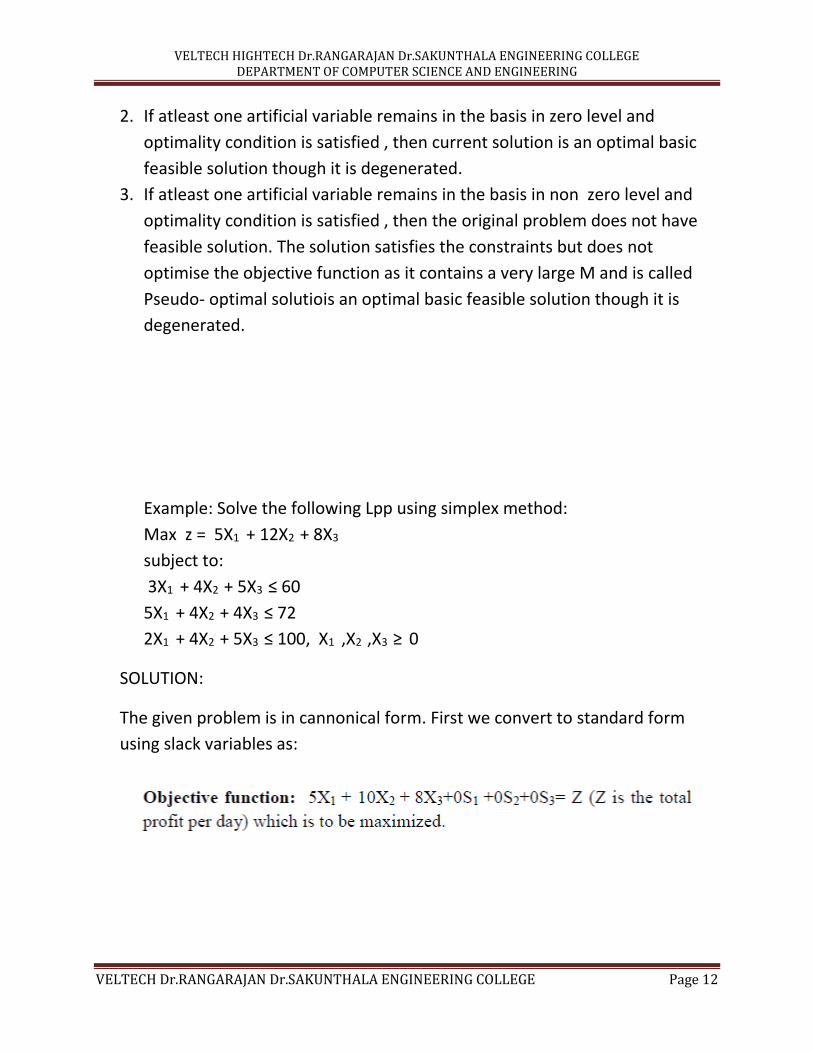
SOLUTION:
The given problem is in cannonical form. First we convert to standard form
using slack variables as:

VELTECH HIGHTECH Dr.RANGARAJAN Dr.SAKUNTHALA ENGINEERING COLLEGE DEPARTMENT OF COMPUTER SCIENCE AND ENGINEERING
VELTECH Dr.RANGARAJAN Dr.SAKUNTHALA ENGINEERING COLLEGE Page 13
There are 6 variables and 3 equation therefore 6 – 3 = 3, 3 variables have to be
made as zeros and the are x1 , x2, x3 = 0 which when substituted in (ii) we get
the basic solution as s1 = 60. s2 = 72, s3 = 100 called the basic solution and
is the basis of the problem. We us iterative method to solve now:
Initial iteration:
Using the method as explained before we can get the first oteration as :
VELTECH HIGHTECH Dr.RANGARAJAN Dr.SAKUNTHALA ENGINEERING COLLEGE DEPARTMENT OF COMPUTER SCIENCE AND ENGINEERING
VELTECH Dr.RANGARAJAN Dr.SAKUNTHALA ENGINEERING COLLEGE Page 14
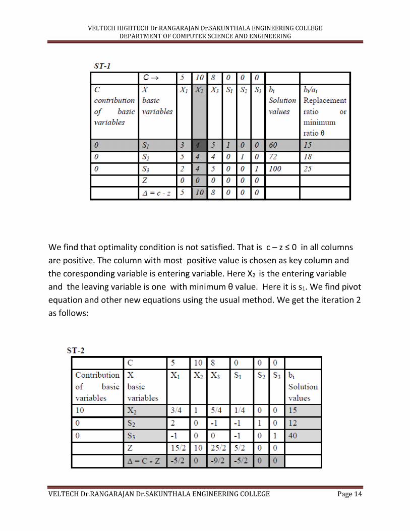
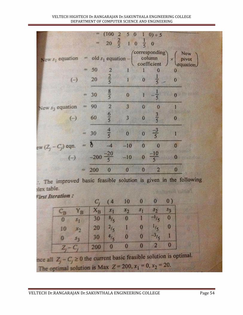
We find that optimality condition is not satisfied. That is c – z ≤ 0 in all columns
are positive. The column with most positive value is chosen as key column and
the coresponding variable is entering variable. Here X2 is the entering variable
and the leaving variable is one with minimum θ value. Here it is s1. We find pivot
equation and other new equations using the usual method. We get the iteration 2
as follows:
VELTECH HIGHTECH Dr.RANGARAJAN Dr.SAKUNTHALA ENGINEERING COLLEGE DEPARTMENT OF COMPUTER SCIENCE AND ENGINEERING
VELTECH Dr.RANGARAJAN Dr.SAKUNTHALA ENGINEERING COLLEGE Page 15
We observe that C – Z ≤ 0 in all columns, therefore optimal solution has been
obtained. Solution is Max Z = 5 x 0 + 12 x 15 + 8 x 0 = 180.
Sensitivity Analysis: This is the study of changes in the optimal solution
when
1. Ther is deletion and adition of new constraints.
2. Change in the values of coefficients in the objective function
3. Coefficients of variables in the constraints change.
4. The right handside constants of the constraints change..
Variation affecting the feasibility :
Two types of changes that could affect the current feasibility solution are:
1. Change in resources availability
2. Addition of constraints.
3. Any change in b will not affect the ZJ - cJ as it is optimal condition not
involving b’s. XB = B- (b) depends upon b therefore change in b will afect
feasibility of current solution
4. Addition of new constraints cannot improve the optimal value of any LPP
5. If new constraint is satisfied by current optimal solution , then the new
constraint is called REDUNTANT constraint as its addition will not change
the solution i.e current solution is feasiblblw and optimal.
UNIT II
If the given LPP is called as PRIMAL ( dual ) problem then this changed to
another problem with optimisation opposite to the given problem and
constraints changed is called the Dual problem( primal )
If the given problem is maximisation ( minimisation) then its dual will be
minimisation ( maximisation )
VELTECH HIGHTECH Dr.RANGARAJAN Dr.SAKUNTHALA ENGINEERING COLLEGE DEPARTMENT OF COMPUTER SCIENCE AND ENGINEERING
VELTECH Dr.RANGARAJAN Dr.SAKUNTHALA ENGINEERING COLLEGE Page 16
If there are n variables and m equations in primal then in its dualthere will be
m variables and n equations.
In the primal maximisation ( minimisation ) all the constraints have to be ≤ ( all
the constraints have to be ≥ ) . Its dual minisation ( maximisation ) will have all
its constraints ≥ (all the constraints have to be ≤ )
If in the primal x3 is unrestricted then in the dual third constraint is a
equality.If in the primal 4th constraint is equality then in dual fourth variable is
unrestricted.
Differentiate between Simplex method and dual simplex method.
1. In Simplex method feasible solution may be ther but optimality condition
wll not be satisfied.
In Dual simplex method the solution is be infeasible but optimality
condition is not satisfied.
2. W e find the entering variable first in the iteration table in the case of
simplex method by considering the most negetive of Zj - Cj , called the key
column and then the leaving variable by considering the minimum of θ ,
where θ = Min [𝑋𝐵𝑖
𝑎𝑖𝑟 ] where XBi refers to ith row of XB column and air refers
to element in XBi th row in the key column. The variable with respect to
this element is the entering variable and the row is called the key row.
3. W e find the leaving variable first in the iteration table in the case of dual
simplex method by considering the most negetive of XBi ‘s , called the key
row and then the entering variable by considering the maximum of θ ,
where θ = Max [𝑍𝑗− 𝐶𝑗
𝑎𝑘𝑗 ] where XBi refers to ith row of XB column and akj
refers to element in XBi th row of Zj - Cj th column . The variable with most
negetive in XB column is leaving variable and entering variable is with max
of θ.
Transportation Problem:
VELTECH HIGHTECH Dr.RANGARAJAN Dr.SAKUNTHALA ENGINEERING COLLEGE DEPARTMENT OF COMPUTER SCIENCE AND ENGINEERING
VELTECH Dr.RANGARAJAN Dr.SAKUNTHALA ENGINEERING COLLEGE Page 17
A transportation is a minimisation problem and is an LPP. There are m
sources and n destination and commodities are transported from every source
to every other destination. The assumptions are :
1. The availability of commodities in each source and the requirement in
every destination
2. The unit cost of transportation from each source to every other destination.
If Cij refers to unit cost of transportation from ith source to jth destination
and xij refers to alloction ith source to jth destination , the total cost of
transportation from ith source to jth destination is Cij xij . The RIM condition is
that sum of supplies in any source (row) is equal to the availability in that
source and the sum of demands in any destinnation (column ) is equal to the
requirement at that destination. With this as constraint the LPP of TP is given
by:
Minimisation Z = ∑ ∑ 𝑐𝑖𝑗𝑥𝑖𝑗𝑛1
𝑚1
Subject to conditions ∑ 𝑥𝑖𝑗𝑛1 = ai I = 1,2,…………..m
∑ 𝑥𝑖𝑗𝑚11 = bj j = 1,2,…………..n
Xij ≥ 0
Points to be remembered while working out a problem on TP:
1. Check whether the TP is balanced in the sense that Sum of the supplies is
equal to sum of the demands i.e ∑ 𝑎𝑖𝑚1 = ∑ 𝑏𝑗
𝑛1
2. Find the solution to the TP which is nothing but finding the allocations from
sources to destinations. The solutions so obtained should satisfy the RIM
conditions namely:
∑ 𝑥𝑖𝑗𝑛1 = ai I = 1,2,…………..m
∑ 𝑥𝑖𝑗𝑚11 = bj j = 1,2,…………..n. The number of allocations should not be
more m+ n+ 1 where m refers to number of rows and n refers to number of
columns.
VELTECH HIGHTECH Dr.RANGARAJAN Dr.SAKUNTHALA ENGINEERING COLLEGE DEPARTMENT OF COMPUTER SCIENCE AND ENGINEERING
VELTECH Dr.RANGARAJAN Dr.SAKUNTHALA ENGINEERING COLLEGE Page 18
3. By feasible solution of a TP we mean the non negetive allocations that
satisfy rim conditions. If the number of allocations do not exceed m+ n+ 1
where m refers to number of rows and n refers to number of columns. i.e
Xij ≥ 0 for all i and j then it is called as basic feasible solution
4. Optimal solution of a TP: It is the feasible solution of the TP which minises
the obejective function viz the cost of transportation.
5. An initial basic fesible solution(ibfs) is said to be non degenerative or the
given TP is said to be a problem of non-degeneration if the number of
allocations is exactly equal to m+ n+ 1.
6. The ibfs of a TP is said to be degenerative or it is a problem of
degeneration if the number of allocation is less than m+ n+ 1.
7. The method to overcome problem of degeneracy: This degeneracy problem
is overcome by assigning the very small quantity ( allocation ) ∈ ≥ 0 to any
one of the independent cells. After finding the ibfs , allow ∈ to tend to zero
and obtain the cost of TP.
8. We say the allocations are in independent cells if it is impossible to increase
or decrease any allocation without either changing the position of
allocation orviolating the rim conditions.
9. The three methods employed to solve a TP are:
(i). North West Corner Method ( nwcm)
(ii) Least Cost Method (lcm)
(iii) Vogel’s Approximation Method (VAM)
North West Corner Method:
1. Choose Cell (1 1) , the nwc cell . Allocate to this cell Min( supply demand ).
Close that row or column if full availability or full demand is met. Round off
the full allocate figure, simultanesoult reduce the higher figure to that

VELTECH HIGHTECH Dr.RANGARAJAN Dr.SAKUNTHALA ENGINEERING COLLEGE DEPARTMENT OF COMPUTER SCIENCE AND ENGINEERING
VELTECH Dr.RANGARAJAN Dr.SAKUNTHALA ENGINEERING COLLEGE Page 19
exten. ( in case both are same both the rows and columns, which will result
in degeneracy )
2. Rewrite the remaining matrix and repeat the process as in 1.
3. Continue this till full allocations are made . These allocations form the ibfs.
The initial cost is obtained by adding the allocations with their respective
unit cost of transportation
Least Cost method:
The cell with the least transportation cost is chosen. As in NWCM the
allocation is made. After closing the row or column ( or both – degeneracy ) the
remaining matrixis formed and the process is repeated till all the alocations are
made.
Vogel’s Approximation Method (VAM): This is called as penalty method. The
penalties are nothing but the difference between the least cost in a row(or
column ) and the next least cost. Penalty is found for every row and coulmn in the
cost matrix. The row ( or coumn ) with maximum penalty is chosen. As in
previous two methods , the least cost cell is chosen in that row( or column ) and
allocated to this cell the minimum of supply and demand and that row or column
is closed . The full allocation is rounded off and the higher figure is reduced to
that extent. The process of finding penaltyand allocation accordingly are carried
out till all allocations are done.
We may notice that the initial basic transportation using VAM < the initial basic
transportation using LCM < the initial basic transportation using NWCM.
MODIFIED DISTRIBUTION METHOD or called as Modi method is u – v method:
Steps involved are:
1. This method is applied in order to find the optimal solution to the given TP.
After finding the ibfs, we assign variables u1, u2, ……………. Un.to rows and
v1, v2, ……………. Vm. to columns. The ui or vj is assigned the value zero
whose row or column has the maximum number of allocations.
VELTECH HIGHTECH Dr.RANGARAJAN Dr.SAKUNTHALA ENGINEERING COLLEGE DEPARTMENT OF COMPUTER SCIENCE AND ENGINEERING
VELTECH Dr.RANGARAJAN Dr.SAKUNTHALA ENGINEERING COLLEGE Page 20
2. Now keeping allocated cells as reference , the values for the remaining u’s
and v’s are found using the formula uij + vij = Cij for all i and j.
3. For the unallocated cells two quantities are determined. One is uij + vij =
Cij and the other is dij = Cij - ( uij + vij ) for all I and j
OBSERVATIONS on dij :
(i) If dij ≥ 0 then the solution obtained is optimal.
(ii) If dij = 0 for some i and j the solution is optimal but alternative
solution exists.
(iii) If dij < 0 atleast for one i and j, then the solution is not optimal and
this cell will be allocated the maximum by a looping method which is
explained as below:
Assign the maximum +θ to this cell. Join this cell with other allocated
cells using horizontal and vertical lines. Assign -θ, +θ, -θ, +θ
alternately to cells which form the corners. Choose the minimum of
all allocations in –θ cells . Add this with the allocation in the +θ cell
allocation and subtract this from allocation in –θ cell. Note that the
reallocation is made without disturbing the rim conditions.
Perfom now the MODI test If all dij ≥ 0 then the solution obtained is
optimal if not repeat the process to get optimal solution
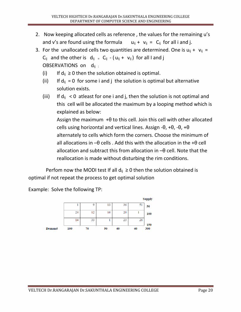
Example: Solve the following TP:

VELTECH HIGHTECH Dr.RANGARAJAN Dr.SAKUNTHALA ENGINEERING COLLEGE DEPARTMENT OF COMPUTER SCIENCE AND ENGINEERING
VELTECH Dr.RANGARAJAN Dr.SAKUNTHALA ENGINEERING COLLEGE Page 21
ASSIGNMENT PROBLEM:

VELTECH HIGHTECH Dr.RANGARAJAN Dr.SAKUNTHALA ENGINEERING COLLEGE DEPARTMENT OF COMPUTER SCIENCE AND ENGINEERING
VELTECH Dr.RANGARAJAN Dr.SAKUNTHALA ENGINEERING COLLEGE Page 22
This is similar to TP. Here there are n jobs and n persons . All the n persons can
perform all the n jobs . This is one job one person optimisation problem . Here it
is assignment of jobs to persons in such a way that the overall time consumed for
completion of jobs orthe overall cost for performing the job is kept
minimum.Unlike the TP assignment problem is always a problem of degeneration
as it is n xn matrix . in TP the number of allocations are 2n – 1 for degneration but
the number of solutions for AP is n only .
The method employed is Hungarian method:
1. Check whether the problem is balanced , if not balance i.e the number of
jobs must be equal to number of persons.
2. Choose the minimum of every row , subtract it from all other elements in
that row, thereby there will be atleast one zero in every row.
3. Check whether every column has atleast a zero, if not repeat the process
as explained in step2.
4. Now bracket a zero for assignment provided it is the only zero in that row.
If more than one zero are there , defer, go to the next and assign. While
making assignment , the other zeros lying up and down , left and right are
marked. This process is carried out for rows and then the same procedure
is followed for columns. The we would notice all the zeros are either
marked or assigned. If all the jobs are all persons the problem is over and
we get optimal solution.If not the following steps are followed:
(i) Tick the unassigned row( rows)
(ii) Move along that row (rows) and tick that column ( columns ) which
has marked zero.
(iii) Move along the ticked column ( columns ) and tick that row ( rows )
which has assignment.
(iv) This process is repeated till all assigned rows and marked columns
are ticked.
(v) Lines are drawn over unticked rows and ticked columns thereby we
get minimum number of lines drawn over all the zeros whose
number is equal to the present assignment.
VELTECH HIGHTECH Dr.RANGARAJAN Dr.SAKUNTHALA ENGINEERING COLLEGE DEPARTMENT OF COMPUTER SCIENCE AND ENGINEERING
VELTECH Dr.RANGARAJAN Dr.SAKUNTHALA ENGINEERING COLLEGE Page 23
(vi) The minimum of open numbers is chosen. This is subtracted from all
other open numbers and added with those numbers at the
intersection of lines. The other numbers are left undisturbed.
(vii) The assignments are made in the same way as explained above.If all
the jobs are assigned to all the persons the problem is over or we
pass onto next iteration starting from step (v) till we get all the jobs
assigned to persons .
The masthematical formulation of the Assignment Problem is
Minimisation Z = ∑ ∑ 𝑐𝑖𝑗𝑥𝑖𝑗𝑛1
𝑚1
Subject to conditions ∑ 𝑥𝑖𝑗𝑛1 = 1 I = 1,2,…………..n
∑ 𝑥𝑖𝑗𝑚11 = 1 . j = 1,2,…………..n and Xij ≥ 0 for all I and j.
Here Xij refers to assignment of ith job to jth person and Cij refers to cost of
performing ith job by jth person or time required for doing ith job by the jth
person. Assignment matrix is called the effective matrix as it can be cost or
time matrix. Note that Xij = 0 if ith job cannot be performed by jth person and
Xij = 1 if ith job can be performed by jth person therefore Xij = 0 or Xij = 1.
Therefore AP is an Integer Programming problem, likewise TP also.
Comparison between Transportation Problem and assignment problem:
Note that both TP and AP minimisation problems. In TP it is allocation of
commodities from sources to destinations. In AP it is assignment of jobs to
different persons.
Commodities can be supplied from a source to any number of destination but
sum of allocation must be equal to its availability.Similarly a destination can
get allocation from any number of sources but the sum of demands received
must be equal to its requirement. This is RIM condition. In AP it is one job one
person that sum of assignmenta in any row or column is equal to one.
VELTECH HIGHTECH Dr.RANGARAJAN Dr.SAKUNTHALA ENGINEERING COLLEGE DEPARTMENT OF COMPUTER SCIENCE AND ENGINEERING
VELTECH Dr.RANGARAJAN Dr.SAKUNTHALA ENGINEERING COLLEGE Page 24
The TP should not be a problem of degeneration whereas AP is always a
problem of degeneration because the number of assignments is always leaa
than m+ n+ 1.
Travelling Salesman Problem (TSP):
This is also assignment problem. A salesman is expected to visit n number of
places for doing business. While going from place to place he is not permitted
to visit a place more than once except the place of start or the Head
Quarters.He is supposed to take the shortes route possible. This can be
achieved by assignment only. As and when a person visits a palce , the
question is which is his next place of visit and which is nearest. This will take
care of distance and time.
(a)The salesman has to go through every city exactly once except starting city.
(b)The salesman starts from one city ( head quarters ) and comes back to
same city ( head quarters )
Hence going from one city to same city is not allowed. ( no assignmnts along
the diagonal of the matrix.)
( a) and (b) are usually called the route conditions.
Example:
Solve the following TSP:
Example:
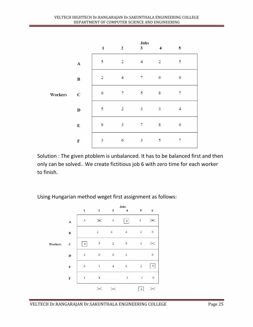
Solve the following AP:
VELTECH HIGHTECH Dr.RANGARAJAN Dr.SAKUNTHALA ENGINEERING COLLEGE DEPARTMENT OF COMPUTER SCIENCE AND ENGINEERING
VELTECH Dr.RANGARAJAN Dr.SAKUNTHALA ENGINEERING COLLEGE Page 25
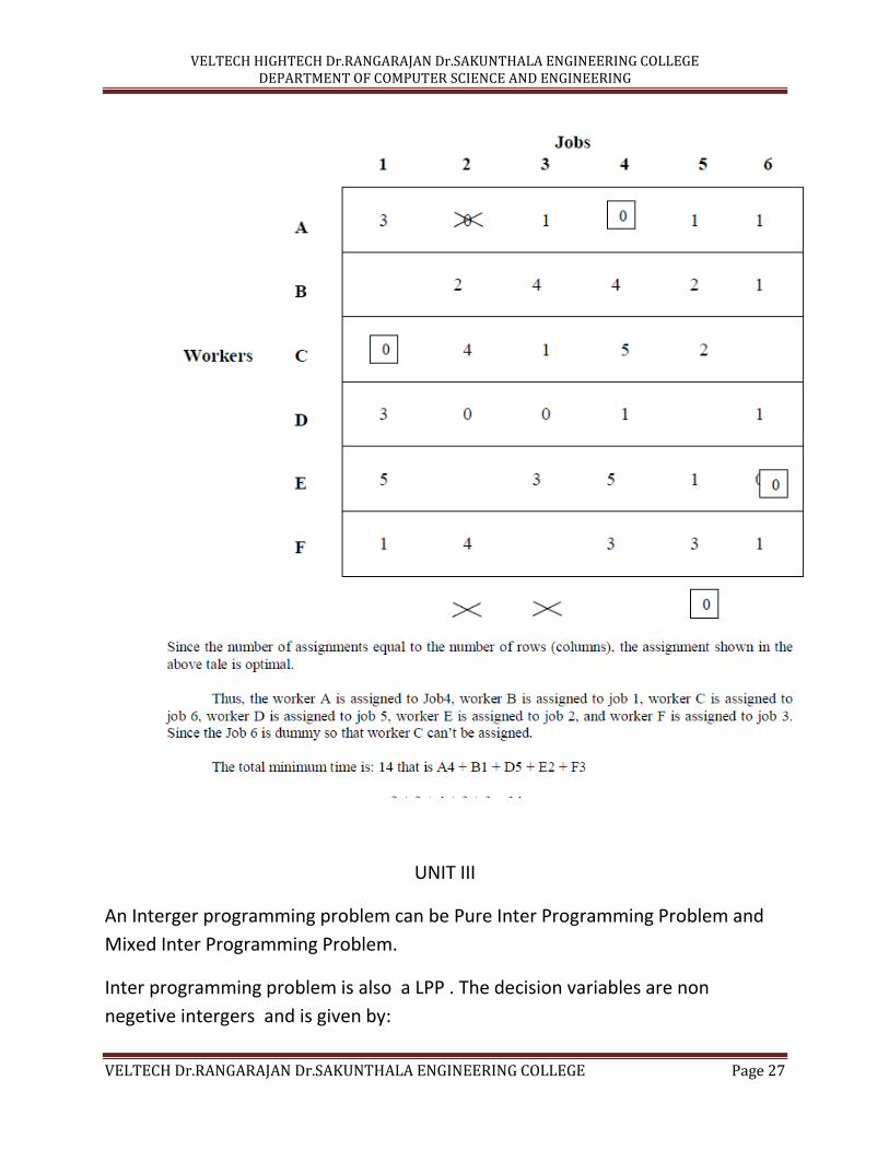
Solution : The given ptoblem is unbalanced. It has to be balanced first and then
only can be solved.. We create fictitious job 6 with zero time for each worker
to finish.
Using Hungarian method weget first assignment as follows:
VELTECH HIGHTECH Dr.RANGARAJAN Dr.SAKUNTHALA ENGINEERING COLLEGE DEPARTMENT OF COMPUTER SCIENCE AND ENGINEERING
VELTECH Dr.RANGARAJAN Dr.SAKUNTHALA ENGINEERING COLLEGE Page 26
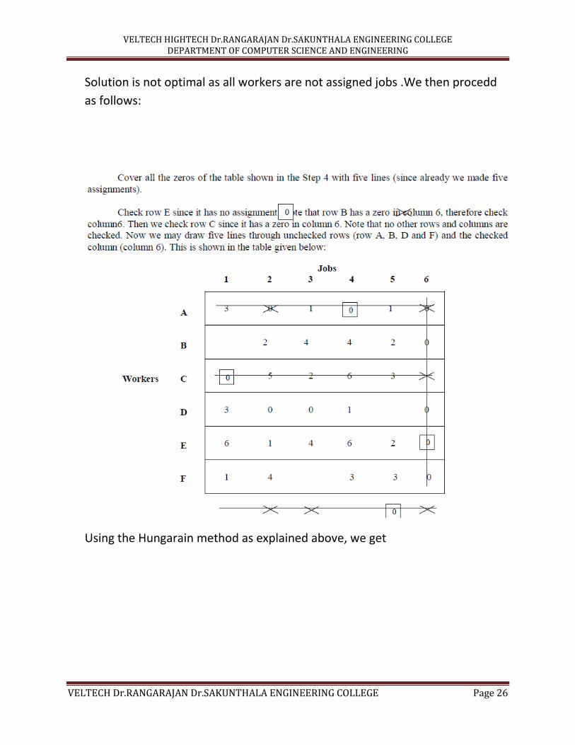
Solution is not optimal as all workers are not assigned jobs .We then procedd
as follows:
Using the Hungarain method as explained above, we get
VELTECH HIGHTECH Dr.RANGARAJAN Dr.SAKUNTHALA ENGINEERING COLLEGE DEPARTMENT OF COMPUTER SCIENCE AND ENGINEERING
VELTECH Dr.RANGARAJAN Dr.SAKUNTHALA ENGINEERING COLLEGE Page 27
UNIT III
An Interger programming problem can be Pure Inter Programming Problem and
Mixed Inter Programming Problem.
Inter programming problem is also a LPP . The decision variables are non
negetive intergers and is given by:
VELTECH HIGHTECH Dr.RANGARAJAN Dr.SAKUNTHALA ENGINEERING COLLEGE DEPARTMENT OF COMPUTER SCIENCE AND ENGINEERING
VELTECH Dr.RANGARAJAN Dr.SAKUNTHALA ENGINEERING COLLEGE Page 28
Maximize Z = f( x1 , x2, x3, ……….. xn)
Subject to constraints:
gj(x1 , x2, x3, ……….. xn ) ≤ = ≥ bj j= 1,2, ………………m.
xi ≥ 0 for all i = 1,2,……………n and are integers.
A mixed ipp is :
Maximize Z = f( x1 , x2, x3, ……….. xn)
Subject to constraints:
gj(x1 , x2, x3, ……….. xn ) ≤ = ≥ bj j= 1,2, ………………m.
xi ≥ 0 for all i = 1,2,……………n and are integers.
Some are variables are restricted to integers and rest can be fractions or
integers.
The pitfalls of rounding decision variable to integer if obtained as decimals.
If the optimal solution obtained as non integer and corrected to nearest in
teger to the lower or higher side then it is likely that it may affect the optimal
solution drastically or the optimal solution will fail to satisfy some of the
constraints.
Two methods are employed to solve ipps in order to overcome such pitfalls.
The methods are:
1. Cutting method
2. Search method
In cutting method or cutting plane method additional constraints are constructed
and introduced with the help of a source row to eliminate the region that does
VELTECH HIGHTECH Dr.RANGARAJAN Dr.SAKUNTHALA ENGINEERING COLLEGE DEPARTMENT OF COMPUTER SCIENCE AND ENGINEERING
VELTECH Dr.RANGARAJAN Dr.SAKUNTHALA ENGINEERING COLLEGE Page 29
not contain integer solution. As many constraints as required are introduced to
eliminate regions which do not give integer solution and solved using dual simplex
method to get integer solution.
Gomorian constraints are introduced systematically using the source row whose
XB value has the maximum fractional part.
The procedure:
1. Convert minimisation LPP to maximisation problem.
2. Solve the LPP using simplex method for optimal solution.
3. If all vaues of decision variables are non negetive integers ,the problem is
over and we have the required solution.
4. If 𝑋𝐵1, 𝑋𝐵2, 𝑋𝐵3, ….. 𝑋𝐵𝑛, are all non integers, the one with maximum
faractional part is chosen as source row say 𝑋𝐵𝑘 = [𝑋𝐵𝑘 ] + fk where [𝑋𝐵𝑘 ]
Is the integral part of 𝑋𝐵𝑘 and fk is the fractional part and 0 < fk < 1. If
the problem is pure IPP, then the GOMORIAN constraint is constructed as
fllows:
Express each of the negetive fractions if any in source row as a negetive
integer plus a non negetive fraction.
∑ 𝑎𝑘𝑗𝑥𝑗 = 𝑋𝐵𝑘
∑{[𝑎𝑘𝑗 ] + 𝑓𝑘𝑗}𝑥𝑗 = [𝑋𝐵𝑘 ] + fk
In the form
∑ 𝑓𝑘𝑗𝑥𝑗 ≥ 𝑓𝑘
Or - ∑ 𝑓𝑘𝑗𝑥𝑗 + g1 = - 𝑓𝑘 , g1 ≥ o caled the Gomorian slack and the
constraint so formed is called the gomorian constraint.
This Constraint is inserted as additiona row in the final iteration where we
found the fractional optimal solution. Now the problem has become dual
simplex problem with infeasible solution and optimality condition is
reached. Now we solve the problem using dual simplex method . As many
Gomorian constraints as required are introduced and the iterations are
solved using dual simplex method till we get integer values for all variables.

VELTECH HIGHTECH Dr.RANGARAJAN Dr.SAKUNTHALA ENGINEERING COLLEGE DEPARTMENT OF COMPUTER SCIENCE AND ENGINEERING
VELTECH Dr.RANGARAJAN Dr.SAKUNTHALA ENGINEERING COLLEGE Page 30
The method employed to solve a MIXED INTER PROGRAMMING PROBLEM
is the same except for construction of Gomorian constraint.
5. Convert minimisation LPP to maximisation problem.
6. Solve the LPP using simplex method for optimal solution.
7. If all vaues of decision variables are non negetive integers ,the problem is
over and we have the required solution.
8. If 𝑋𝐵1, 𝑋𝐵2, 𝑋𝐵3, ….. 𝑋𝐵𝑛, are all non integers, the one with maximum
faractional part is chosen as source row say 𝑋𝐵𝑘 = [𝑋𝐵𝑘 ] + fk where [𝑋𝐵𝑘 ]
Is the integral part of 𝑋𝐵𝑘 and fk is the fractional part and 0 < fk < 1. If
the problem is Mixed IPP, then the GOMORIAN constraint is constructed as
fllows:
Express each of the negetive fractions if any in source row as a negetive
integer plus a non negetive fraction.
∑ 𝑎𝑘𝑗𝑥𝑗 = 𝑋𝐵𝑘
∑{[𝑎𝑘𝑗 ] + 𝑓𝑘𝑗}𝑥𝑗 = [𝑋𝐵𝑘 ] + fk
In the form ∑ 𝑓𝑘𝑗𝑥𝑗 ≥ 𝑓𝑘
∑ 𝑓𝑘𝑗𝑥𝑗𝑗∈𝑗+ + [𝑓𝑘
𝑓𝑘−1 ] ∑ 𝑓𝑘𝑗𝑥𝑗𝑗∈𝑗− ≥ 𝑓𝑘
-∑ 𝑓𝑘𝑗𝑥𝑗𝑗∈𝑗+ - [𝑓𝑘
𝑓𝑘−1 ] ∑ 𝑓𝑘𝑗𝑥𝑗𝑗∈𝑗− ≤ - 𝑓𝑘
-∑ 𝑓𝑘𝑗𝑥𝑗𝑗∈𝑗+ - [𝑓𝑘
𝑓𝑘−1 ] ∑ 𝑓𝑘𝑗𝑥𝑗𝑗∈𝑗− + g1 = - 𝑓𝑘
Where g1 ≥ 0 and the constraint is Gomorian constraint
Where j+ refers to terms which are positive and j- are terms which are
negetive.
Search method: In this the branch and bound method is applied to get the
integer solutions either by graphical method ( if two variables ) and simplex
method otherwise.
In branch and bound method for e.g x1 = 2.75 , it means 2 ≤ x1 ≤ 3.
VELTECH HIGHTECH Dr.RANGARAJAN Dr.SAKUNTHALA ENGINEERING COLLEGE DEPARTMENT OF COMPUTER SCIENCE AND ENGINEERING
VELTECH Dr.RANGARAJAN Dr.SAKUNTHALA ENGINEERING COLLEGE Page 31
It is clear that there is no integer solution in 2< x1 < 3. Therefore we search
for integer solution in regions x1 ≤ 2 and x1 ≥ 3 and these two regions are
mutually disjoint.
Now we have two sub problems with newly formed constraints and we
have to solve the two sub problems . The braching process is continued
until each problems terminates with either interger optimal solution or
there is evidence that it can not yield a better solution. The integer valued
solution among al the sub- problems which gives the most optimum value
of sthe objective function is then selected as the optimum solution.
Main disadvantage of this method is that it requires the optimum solution
of each sub –problem. In large problems this could be very tedious job. But
the computational efficiency osf this method is increased by using the
concept of BOUNDING. By this concept whenever the continuous optimum
solution of a sub-problem yields a value of the objective function lower
than that of the best available solution ( for maximisation problem ) it is
useless to explore the problem any further. This problem is said to be
fathomed and is dropped from further consideration. Thus once a feasible
inter solution is obtained , its associated objective function can be taken
as the LOWER BOUND ( for maximisation problem ) to give inferior sub
problems. Hence efficiency of a branch and bound method depends upon
the successive sub problems are found.
For minimisation problem instead of lower bound upp bound is
considered.
Example: Use Branch and Bound technique to solve the following LPP for
integer values:
2.) Solve the following IPP:
Min Z = -2X1 - 3X2 , subject to:
2X1 + 2X2 ≤ 57
X1 ≤ 2, X2 ≤ 2, X1 , X2 ≥ 0 and are integers.
Solution: Convert to Maximisation problem as :
VELTECH HIGHTECH Dr.RANGARAJAN Dr.SAKUNTHALA ENGINEERING COLLEGE DEPARTMENT OF COMPUTER SCIENCE AND ENGINEERING
VELTECH Dr.RANGARAJAN Dr.SAKUNTHALA ENGINEERING COLLEGE Page 32
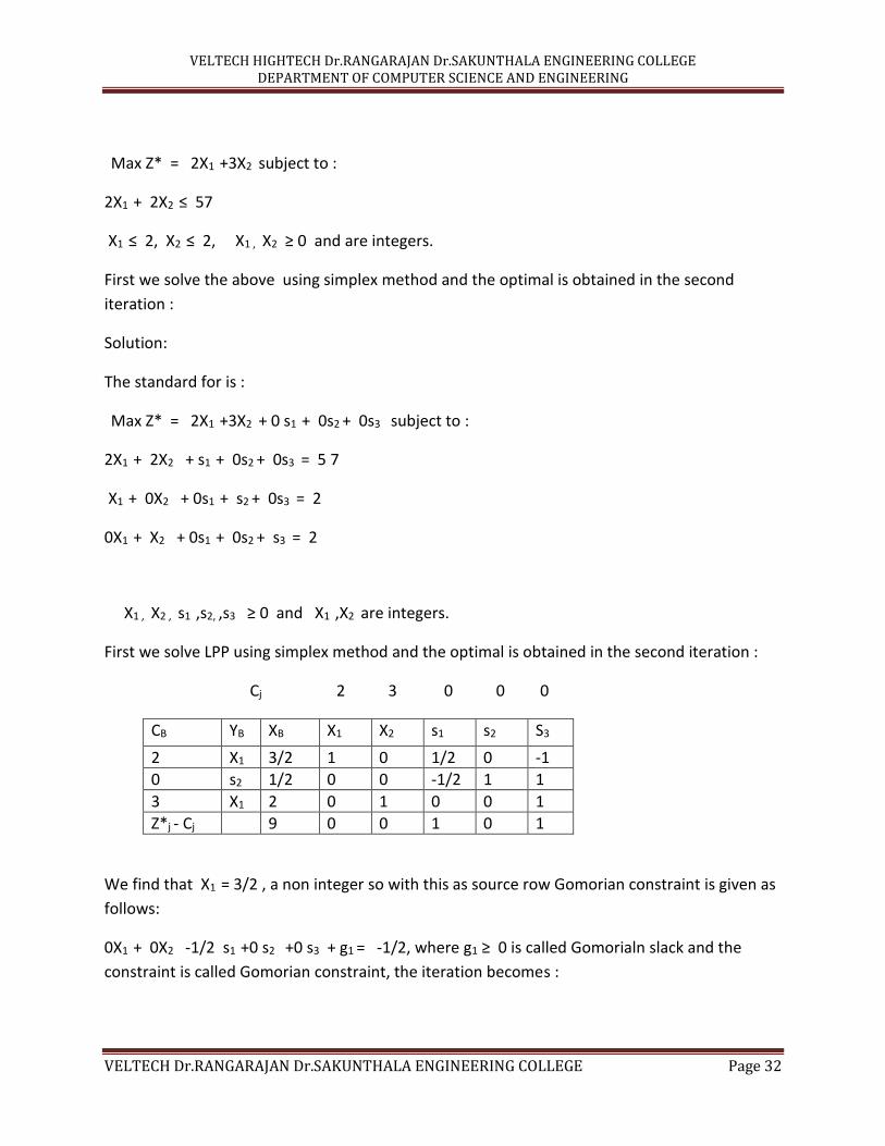
Max Z* = 2X1 +3X2 subject to :
2X1 + 2X2 ≤ 57
X1 ≤ 2, X2 ≤ 2, X1 , X2 ≥ 0 and are integers.
First we solve the above using simplex method and the optimal is obtained in the second
iteration :
Solution:
The standard for is :
Max Z* = 2X1 +3X2 + 0 s1 + 0s2 + 0s3 subject to :
2X1 + 2X2 + s1 + 0s2 + 0s3 = 5 7
X1 + 0X2 + 0s1 + s2 + 0s3 = 2
0X1 + X2 + 0s1 + 0s2 + s3 = 2
X1 , X2 , s1 ,s2, ,s3 ≥ 0 and X1 ,X2 are integers.
First we solve LPP using simplex method and the optimal is obtained in the second iteration :
Cj 2 3 0 0 0
CB YB XB X1 X2 s1 s2 S3
2 X1 3/2 1 0 1/2 0 -1
0 s2 1/2 0 0 -1/2 1 1
3 X1 2 0 1 0 0 1
Z*j - Cj 9 0 0 1 0 1
We find that X1 = 3/2 , a non integer so with this as source row Gomorian constraint is given as
follows:
0X1 + 0X2 -1/2 s1 +0 s2 +0 s3 + g1 = -1/2, where g1 ≥ 0 is called Gomorialn slack and the
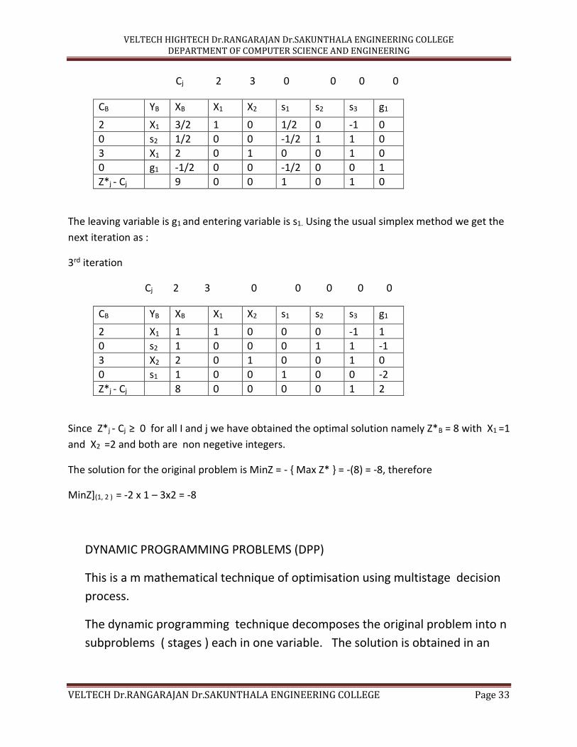
constraint is called Gomorian constraint, the iteration becomes :
VELTECH HIGHTECH Dr.RANGARAJAN Dr.SAKUNTHALA ENGINEERING COLLEGE DEPARTMENT OF COMPUTER SCIENCE AND ENGINEERING
VELTECH Dr.RANGARAJAN Dr.SAKUNTHALA ENGINEERING COLLEGE Page 33
Cj 2 3 0 0 0 0
CB YB XB X1 X2 s1 s2 s3 g1
2 X1 3/2 1 0 1/2 0 -1 0
0 s2 1/2 0 0 -1/2 1 1 0
3 X1 2 0 1 0 0 1 0
0 g1 -1/2 0 0 -1/2 0 0 1
Z*j - Cj 9 0 0 1 0 1 0
The leaving variable is g1 and entering variable is s1. Using the usual simplex method we get the
next iteration as :
3rd iteration
Cj 2 3 0 0 0 0 0
CB YB XB X1 X2 s1 s2 s3 g1
2 X1 1 1 0 0 0 -1 1
0 s2 1 0 0 0 1 1 -1
3 X2 2 0 1 0 0 1 0
0 s1 1 0 0 1 0 0 -2
Z*j - Cj 8 0 0 0 0 1 2
Since Z*j - Cj ≥ 0 for all I and j we have obtained the optimal solution namely Z*B = 8 with X1 =1
and X2 =2 and both are non negetive integers.
The solution for the original problem is MinZ = - { Max Z* } = -(8) = -8, therefore
MinZ](1, 2 ) = -2 x 1 – 3x2 = -8
DYNAMIC PROGRAMMING PROBLEMS (DPP)
This is a m mathematical technique of optimisation using multistage decision
process.
The dynamic programming technique decomposes the original problem into n
subproblems ( stages ) each in one variable. The solution is obtained in an
VELTECH HIGHTECH Dr.RANGARAJAN Dr.SAKUNTHALA ENGINEERING COLLEGE DEPARTMENT OF COMPUTER SCIENCE AND ENGINEERING
VELTECH Dr.RANGARAJAN Dr.SAKUNTHALA ENGINEERING COLLEGE Page 34
ordinary manner by starting from one stage to next and is completed after the
final is reached.
Bellman’s principle of optimality:
An optimal policy ( set of decisions ) has the property that whatever be the
initial state and initial decisions, the remaining decisions must constitute an
optimal policy for the state resulting from the first decision.
It states that given the initial state of the system an optimal policy for the
subsquent stages does not depend upon the policy adopted at the preceeding
stages.
Characteristics of DPP:
1. Problem can be divided into stages , with policy decision required at each
stage.
2. Sttes are associated with each stage may be finite or infinite.
3. Of policy decision at a stage is change the state to next state in next
stage.
4. Current situation is described by a set of secision variables.
5. Given the current state or optimal policy for remaining stages is
independent of the policy adopted in previous stages.
6. The solution procedure begins by finding the optimal policy for each state
of the last stage.
7. A recursive relation ( recurrsive relation or functional equation ) which
identifies the optimal policy for each state with n stages remaining given
the optimal policy for each state with ( n – 1 ) stages left.
8. Using this recursive relationship the solution procedure moves backward
stage by stage, each time finding the policy when starting at the initial
stage.
DPP algorithm:
1. Identify decision variables and the objective function
2. Number of sub problems and identify that state variables at each state.
VELTECH HIGHTECH Dr.RANGARAJAN Dr.SAKUNTHALA ENGINEERING COLLEGE DEPARTMENT OF COMPUTER SCIENCE AND ENGINEERING
VELTECH Dr.RANGARAJAN Dr.SAKUNTHALA ENGINEERING COLLEGE Page 35
3. Write the general recursive relationship for computing optimal policy.
4. Write the reltion giving the optimal decision function for one stage sub
problem and solve it.
5. Solve the optimal decision function for 2-stage, 3-stage….. ( n-1 ) stage and
n- stage problem.
If the DPP is solved using the recursive equation . starting from the first
through the last stage i.e obtaining a sequence
f1 → f2 → f3 ………………………………………….. → fn of the optimal solution . This
equation is called the forward computational procedure.
If the recursive equation are formulated to obtain a sequence as gibrn
here fn → fn-1 → fn-2 ………………………………………….. → f1 then the computation is
called backward computational procedure.
Applications of DPP:
1. It is applied in production area- production sheduling and employment
smoothening problems .
2. In deterministic inventory problems.
3. Allocation of different salesman to different places for optimisation of
sales.
4. To determine the optimal combination of advertising media (TV, Radio.
Paper)and the frequency of advertising.
Example:
Optimal sub division problem:
Divide the quantity c into n parts such a way that their product is maximum. That divide c into
y1, y2, ………………….., yn parts such that
Maximum Z = y1 X y2 X …………………..X yn subject to constraints:
y1 + y2 + …………………..+ yn = c
Solution:
We develop a recursive equation to solve the problem.
VELTECH HIGHTECH Dr.RANGARAJAN Dr.SAKUNTHALA ENGINEERING COLLEGE DEPARTMENT OF COMPUTER SCIENCE AND ENGINEERING
VELTECH Dr.RANGARAJAN Dr.SAKUNTHALA ENGINEERING COLLEGE Page 36
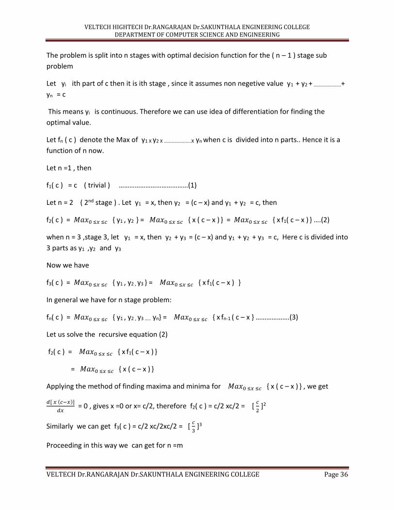
The problem is split into n stages with optimal decision function for the ( n – 1 ) stage sub
problem
Let yi ith part of c then it is ith stage , since it assumes non negetive value y1 + y2 + …………………..+
yn = c
This means yi is continuous. Therefore we can use idea of differentiation for finding the
optimal value.
Let fn ( c ) denote the Max of y1 X y2 X …………………..X yn when c is divided into n parts.. Hence it is a
function of n now.
Let n =1 , then
f1( c ) = c ( trivial ) …………………………………(1)
Let n = 2 ( 2nd stage ) . Let y1 = x, then y2 = (c – x) and y1 + y2 = c, then
f2( c ) = 𝑀𝑎𝑥0 ≤𝑥 ≤𝑐 { y1 , y2 } = 𝑀𝑎𝑥0 ≤𝑥 ≤𝑐 { x ( c – x ) } = 𝑀𝑎𝑥0 ≤𝑥 ≤𝑐 { x f1( c – x ) } ….(2)
when n = 3 ,stage 3, let y1 = x, then y2 + y3 = (c – x) and y1 + y2 + y3 = c, Here c is divided into
3 parts as y1 ,y2 and y3
Now we have
f3( c ) = 𝑀𝑎𝑥0 ≤𝑥 ≤𝑐 { y1 , y2 , y3 } = 𝑀𝑎𝑥0 ≤𝑥 ≤𝑐 { x f1( c – x ) }
In general we have for n stage problem:
fn( c ) = 𝑀𝑎𝑥0 ≤𝑥 ≤𝑐 { y1 , y2 , y3 ….. yn} = 𝑀𝑎𝑥0 ≤𝑥 ≤𝑐 { x fn-1 ( c – x } ……………….(3)
Let us solve the recursive equation (2)
f2( c ) = 𝑀𝑎𝑥0 ≤𝑥 ≤𝑐 { x f1( c – x ) }
= 𝑀𝑎𝑥0 ≤𝑥 ≤𝑐 { x ( c – x ) }
Applying the method of finding maxima and minima for 𝑀𝑎𝑥0 ≤𝑥 ≤𝑐 { x ( c – x ) } , we get
𝑑[ 𝑥 (𝑐−𝑥)]
𝑑𝑥 = 0 , gives x =0 or x= c/2, therefore f2( c ) = c/2 xc/2 = [
𝑐
2 ]2
Similarly we can get f3( c ) = c/2 xc/2xc/2 = [ 𝑐
3 ]3
Proceeding in this way we can get for n =m
VELTECH HIGHTECH Dr.RANGARAJAN Dr.SAKUNTHALA ENGINEERING COLLEGE DEPARTMENT OF COMPUTER SCIENCE AND ENGINEERING
VELTECH Dr.RANGARAJAN Dr.SAKUNTHALA ENGINEERING COLLEGE Page 37
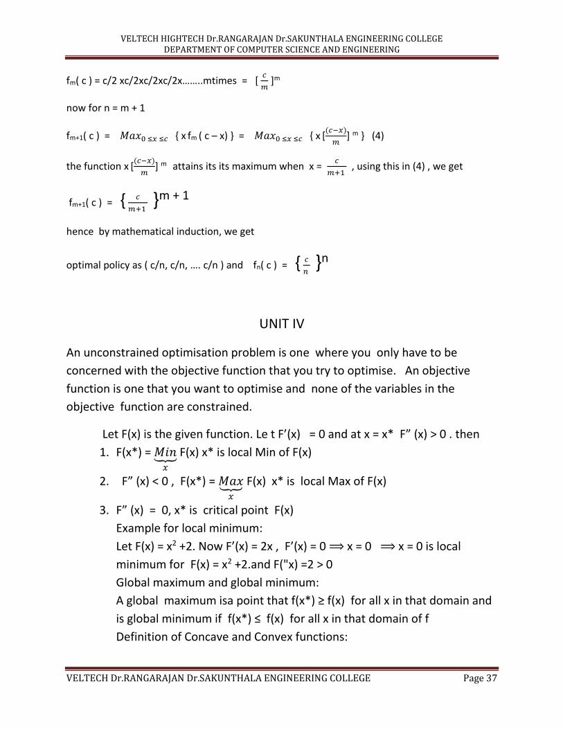
fm( c ) = c/2 xc/2xc/2xc/2x……..mtimes = [ 𝑐
𝑚 ]m
now for n = m + 1
fm+1( c ) = 𝑀𝑎𝑥0 ≤𝑥 ≤𝑐 { x fm ( c – x) } = 𝑀𝑎𝑥0 ≤𝑥 ≤𝑐 { x [(𝑐−𝑥)
𝑚] m } (4)
the function x [(𝑐−𝑥)
𝑚] m attains its its maximum when x =
𝑐
𝑚+1 , using this in (4) , we get
fm+1( c ) = { 𝑐
𝑚+1 }m + 1
hence by mathematical induction, we get
optimal policy as ( c/n, c/n, …. c/n ) and fn( c ) = { 𝑐
𝑛 }n
UNIT IV
An unconstrained optimisation problem is one where you only have to be
concerned with the objective function that you try to optimise. An objective
function is one that you want to optimise and none of the variables in the
objective function are constrained.
Let F(x) is the given function. Le t F’(x) = 0 and at x = x* F” (x) > 0 . then
1. F(x*) = 𝑀𝑖𝑛⏟𝑥
F(x) x* is local Min of F(x)
2. F” (x) < 0 , F(x*) = 𝑀𝑎𝑥⏟𝑥
F(x) x* is local Max of F(x)
3. F” (x) = 0, x* is critical point F(x)
Example for local minimum:
Let F(x) = x2 +2. Now F’(x) = 2x , F’(x) = 0 ⟹ x = 0 ⟹ x = 0 is local
minimum for F(x) = x2 +2.and F("x) =2 > 0
Global maximum and global minimum:
A global maximum isa point that f(x*) ≥ f(x) for all x in that domain and
is global minimum if f(x*) ≤ f(x) for all x in that domain of f
Definition of Concave and Convex functions:
VELTECH HIGHTECH Dr.RANGARAJAN Dr.SAKUNTHALA ENGINEERING COLLEGE DEPARTMENT OF COMPUTER SCIENCE AND ENGINEERING
VELTECH Dr.RANGARAJAN Dr.SAKUNTHALA ENGINEERING COLLEGE Page 38
When f”(x) ≥ 0 for all x then f(x) is a convex function . Here local
minimum of x* is the global minimum of f(x) .
When f”(x) ≤ 0 for all x then f(x) is a concave function . Here local
maximum f x* is the global maximum of f(x)
The conditions for a minimum or a maximum value of a function of
several variables :
Let f(x) be a function of several independent variables of x .
1. Find ∇ f(x) =0
2. Solve to get the solution vector x*
3. Calculate ∇2 f(x)
4. Evauate at x*
5. Inspect Hessian matrix at x*
H(x) = ∇2 f(x)
The above is symetric matrix .
OBSERVATION and Inferences:
(i) If Hessian matrix H(x*) is positive definite then at x* f(x) has local
minimum at x*.
(ii) If Hessian matrix H(x*) is negetive definite then at x* f(x) has local
maximum at x*.
(iii) If Hessian matrix H(x*) is indefinite matrix then at x* f(x) has
neither local minimum nor local maximum..
If a maximization problem is given as
Max Z = f( x1 , x2, x3, ……….. xn)
Subject to
g( x1 , x2, x3, ……….. xn) ≤ b
xi ≥ 0 for all i = 1,2,……………n the necessary condition for maximisation
is
VELTECH HIGHTECH Dr.RANGARAJAN Dr.SAKUNTHALA ENGINEERING COLLEGE DEPARTMENT OF COMPUTER SCIENCE AND ENGINEERING
VELTECH Dr.RANGARAJAN Dr.SAKUNTHALA ENGINEERING COLLEGE Page 39
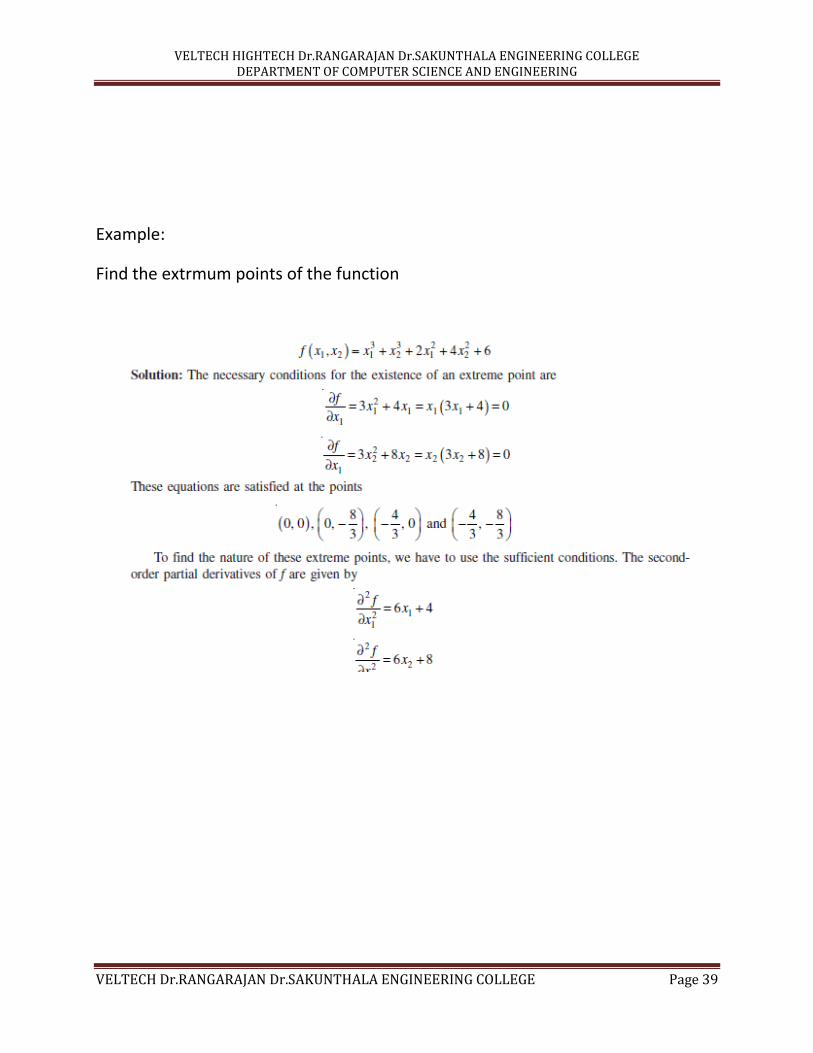
Example:
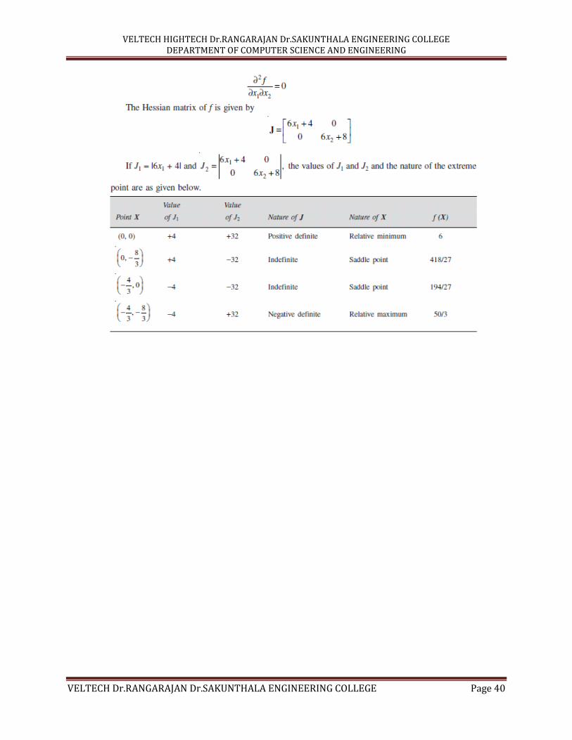
Find the extrmum points of the function
VELTECH HIGHTECH Dr.RANGARAJAN Dr.SAKUNTHALA ENGINEERING COLLEGE DEPARTMENT OF COMPUTER SCIENCE AND ENGINEERING
VELTECH Dr.RANGARAJAN Dr.SAKUNTHALA ENGINEERING COLLEGE Page 40
VELTECH HIGHTECH Dr.RANGARAJAN Dr.SAKUNTHALA ENGINEERING COLLEGE DEPARTMENT OF COMPUTER SCIENCE AND ENGINEERING
VELTECH Dr.RANGARAJAN Dr.SAKUNTHALA ENGINEERING COLLEGE Page 41
UNIT V
A project is defined as a combination of interrelated activities all of which
must be executed in a certain order to achieve goal.
A small project involving very few activities can be efficiently done with
help of experience gained in that field over a period of time. But for a big
project such thumb cannot be used , experience cannot help. A scientific
and mathematical approach is required.
Projects are of two types . They are deterministic projects and the other is
probabilistic projects.
A number of methods applying network scheduling techniques has been
developed.
Programme Evaluation Technique (PERT) and Critical Path Method (CPM)
are two of maany network techniques which commonly used for Plannin,
Scheduling and controlling large complex projects.
The three main manaferial functions for any project are:
1. Planning
2. Scheduling
3. Control.
Planning: This phase involves listing of tasks for the project. We determine
money , men and other resources required for the project. The cost of
project and duration of project is also determined.
Scheduling : We determine in this phase the activities involved in the
project with thwie sequencial order of exection and also the duration of the
project.
Control: This phase consists of reviewing the progress of the project and if
deviations crop they are rectified immediately.Remedial measures are
taken wherever possible without loss of time.
VELTECH HIGHTECH Dr.RANGARAJAN Dr.SAKUNTHALA ENGINEERING COLLEGE DEPARTMENT OF COMPUTER SCIENCE AND ENGINEERING
VELTECH Dr.RANGARAJAN Dr.SAKUNTHALA ENGINEERING COLLEGE Page 42
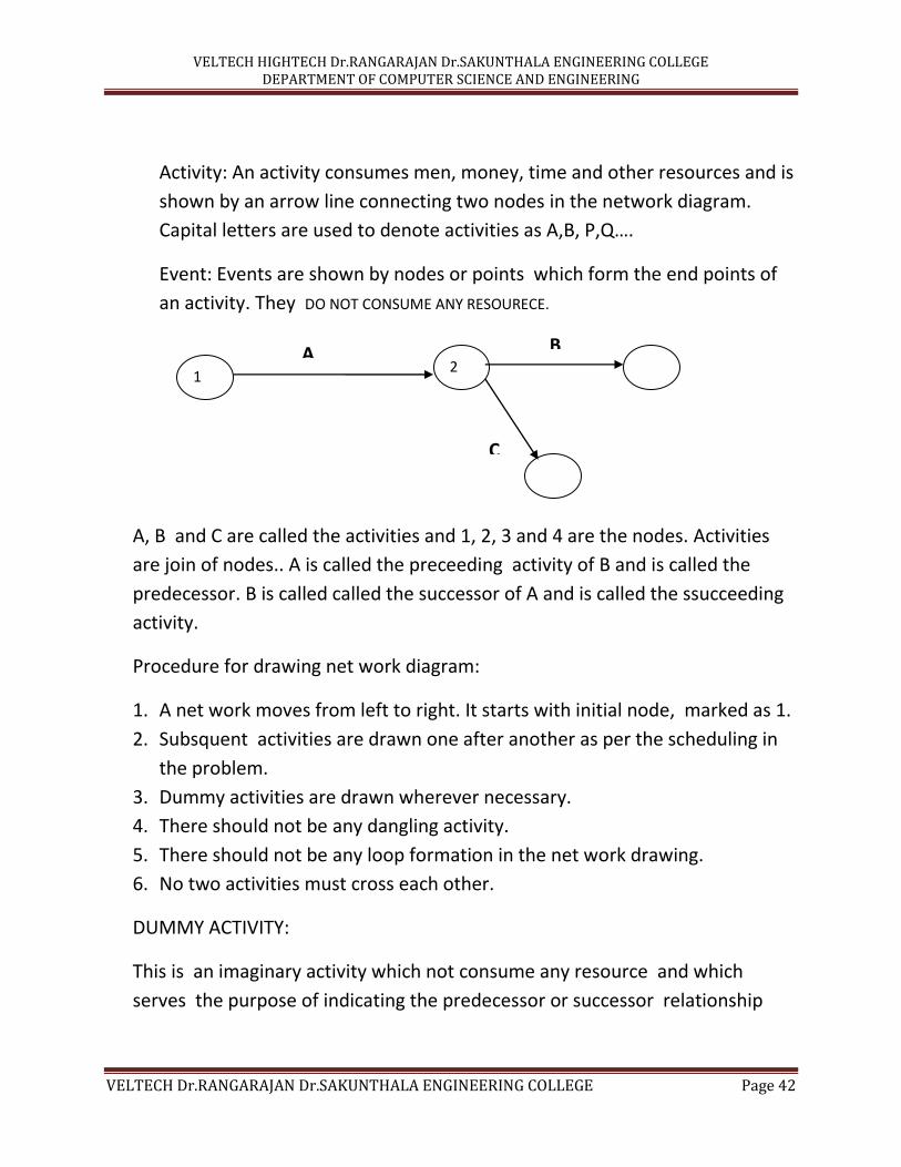
Activity: An activity consumes men, money, time and other resources and is
shown by an arrow line connecting two nodes in the network diagram.
Capital letters are used to denote activities as A,B, P,Q….
Event: Events are shown by nodes or points which form the end points of
an activity. They DO NOT CONSUME ANY RESOURECE.
A, B and C are called the activities and 1, 2, 3 and 4 are the nodes. Activities
are join of nodes.. A is called the preceeding activity of B and is called the
predecessor. B is called called the successor of A and is called the ssucceeding
activity.
Procedure for drawing net work diagram:
1. A net work moves from left to right. It starts with initial node, marked as 1.
2. Subsquent activities are drawn one after another as per the scheduling in
the problem.
3. Dummy activities are drawn wherever necessary.
4. There should not be any dangling activity.
5. There should not be any loop formation in the net work drawing.
6. No two activities must cross each other.
DUMMY ACTIVITY:
This is an imaginary activity which not consume any resource and which
serves the purpose of indicating the predecessor or successor relationship
1 2
A
C
B
VELTECH HIGHTECH Dr.RANGARAJAN Dr.SAKUNTHALA ENGINEERING COLLEGE DEPARTMENT OF COMPUTER SCIENCE AND ENGINEERING
VELTECH Dr.RANGARAJAN Dr.SAKUNTHALA ENGINEERING COLLEGE Page 43
clearly in any activity on arrow diagram. It is merely drawn for techical
completition of the project.
Project Network or Arrow Diagram: Tge diagram denoting all the activities of a
project by arrows taking into account the technological sequence of the
activities is called the project network or arrow diagram.
Fulkerson’s rule for numbering the nodes.
1. Number the start node which has no predecessor activity as 1.
2. Delete all the activities emanating from this node 1.
3. Number all the resulting start nodes without any predecessor as 2,3,..
4. Delete all the activities originating from the start nodes 2,3…in step 3.
5. Number all the resulting new start nodes without any predecessor next to
the last number used in step3.
6. Repeat the process until the terminal node without any successor activity is
reached and number this terminal node suitably.
NETWORK COMPUTATIONS.
We use forward pass calculation to determine Earliest Start Time (EST) . The
EST of an activity i → j in a project network is given by :
ESJ = Max [ESi + tij ] where ESi denotes the earliest start time of all activities
emanating from the node i and tij is the estimated duration of the activity
i → j
We use backward pass calculation to determine Lates Finish Time (LFT) and
Latest Start Time ( LST ) . The LST of an activity i → j in a project network is
given by :
LSi = Min [[LSj - tij ] where tij is the estimated duration activity i → j
Definition of Critical Path: This is a path connecting the initial node to the very
last terminal node , of longest duration in any project net work . ( It is also
defined as path of zero float.)
VELTECH HIGHTECH Dr.RANGARAJAN Dr.SAKUNTHALA ENGINEERING COLLEGE DEPARTMENT OF COMPUTER SCIENCE AND ENGINEERING
VELTECH Dr.RANGARAJAN Dr.SAKUNTHALA ENGINEERING COLLEGE Page 44
Various floats for activities of a project are determined using forward and
backward pass calcularions namely EST AND EFT and LFT and LST.
Total Float of activity i → j is given by:
{ TF ] i→ j = [ LF - EF ] i→ j = [ LS - ES ] i→ j
The Total Float is the amount of time by which the particular activity may be
delayed without affecting the duration of the project.
If TF is greater than zero ( positive quantity )it may mean that the resources
doe that activity is more than enough .
If Total Float of an activity is zero it may mean that the resources available for
the activity is just enough.
If Total Float of an activity is less than zero ( negetive ) it may mean that the
resources available for the activity is just insufficient.
Free Float ( FF ) of activity i → j is given by:
{ FF ] i→ j = [ TF ] i→ j - ( L – E ) of the event j
= [ TF ] i→ j - slack at head j
The significance of Free Float of an activity is that . that particular activity can
be delayed by that much of float without affecting the succeeding activity.
Independent Float ( IF ) of activity i → j is given by:
{ IF ] i→ j = [ FF ] i→ j - ( L – E ) of the event i
= [ FF ] i→ j - slack at tail i
The significance of Independent Float of an activity is that , that particular
activity can be delayed by that much of float without affecting the preceeding
activity.
It is be noted that
VELTECH HIGHTECH Dr.RANGARAJAN Dr.SAKUNTHALA ENGINEERING COLLEGE DEPARTMENT OF COMPUTER SCIENCE AND ENGINEERING
VELTECH Dr.RANGARAJAN Dr.SAKUNTHALA ENGINEERING COLLEGE Page 45
IF ≤ FF ≤ TF
Uses of floats: Floats ar useful in resource levelling and resource allocation
problems. Floats give some flexibility in resheduling
Programme Evaluation Review Technique:
This technique is aplplied to probabilistic projects to determine the critical
path and the different floats.
There are three time estimates, using these we can find one expected time
estimate for every activity . The expected duration of the project is the critical
path. The expected standard deviation of every activity is determined . Using
the standard deviation of critical path we will be determine the probability of
finishing the project before or after the expected duation time.
PERT calculations depend on
1. Optimistic (least) time estimate: ( to or a ) is the duration of any activity
when everything goes on well during the project. That is there wont be any
delay or any difficulty in getting any resource required for the project.
Scarcity of raw materials will not there.
2. Pessimistic ( greatest ) time estimate: ( tp or b ) This is the duration of any
activity when every thing goes against the will of the person doing the
project. He faces all types of difficulties during project execution.
3. Most Likely time estimate: (tm or m ) This is time duration of a project
when things go sometimes well and sometimes bad during the project
execution.
Two main assumptions made in PERT calculation are:
1. The duration of activities are independent.i.e the duration of one
activity does not have a bearing on any other activity.
2. The activity duration follows β – distribution.
The procedure for solving a problem in PERT.
1. Draw the project net work.
VELTECH HIGHTECH Dr.RANGARAJAN Dr.SAKUNTHALA ENGINEERING COLLEGE DEPARTMENT OF COMPUTER SCIENCE AND ENGINEERING
VELTECH Dr.RANGARAJAN Dr.SAKUNTHALA ENGINEERING COLLEGE Page 46
2. Compute the duration of every activity using te = (𝑎 + 𝑏 + 4𝑚 )
6
3. Compute EST, EFR; LST and LFT.
4. Determine the Critical path.
5. Compute the expected variance of activity using σ2 = ( 𝑎−𝑏 )2
36
6. Compute the expected standard deviation of pfoject length σ2c and
calculate the standard normal variate 𝑇𝑆 − 𝑇𝐸
𝜎𝐶
WHERE TS IS sprcified time to
complete the priject, TE expected duration of the project for completion
and σc expected S.D of the project length.
7. We can use to calculate completion of project before or after time using
area under normal curve.
Differences between PERT and CPM:
There are three time estimates in PERT whereas in CPM there is only
one time estimate.
PERT is event oriented whereas CPM is activity oriented.
PERT is appliied to R & D projects whereas CPM is applied to projects
involving well known activities of repetitive n nature. ( applied to
construction buikdins, bridges whose time of completion well
determined. )
Example:
The three time estimates ( in months ) of all actvities of a project are
given below:
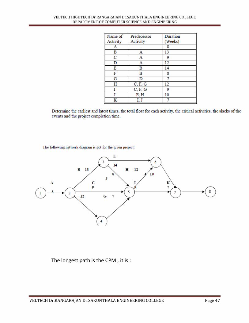
For the following network shedule problem
VELTECH HIGHTECH Dr.RANGARAJAN Dr.SAKUNTHALA ENGINEERING COLLEGE DEPARTMENT OF COMPUTER SCIENCE AND ENGINEERING
VELTECH Dr.RANGARAJAN Dr.SAKUNTHALA ENGINEERING COLLEGE Page 47
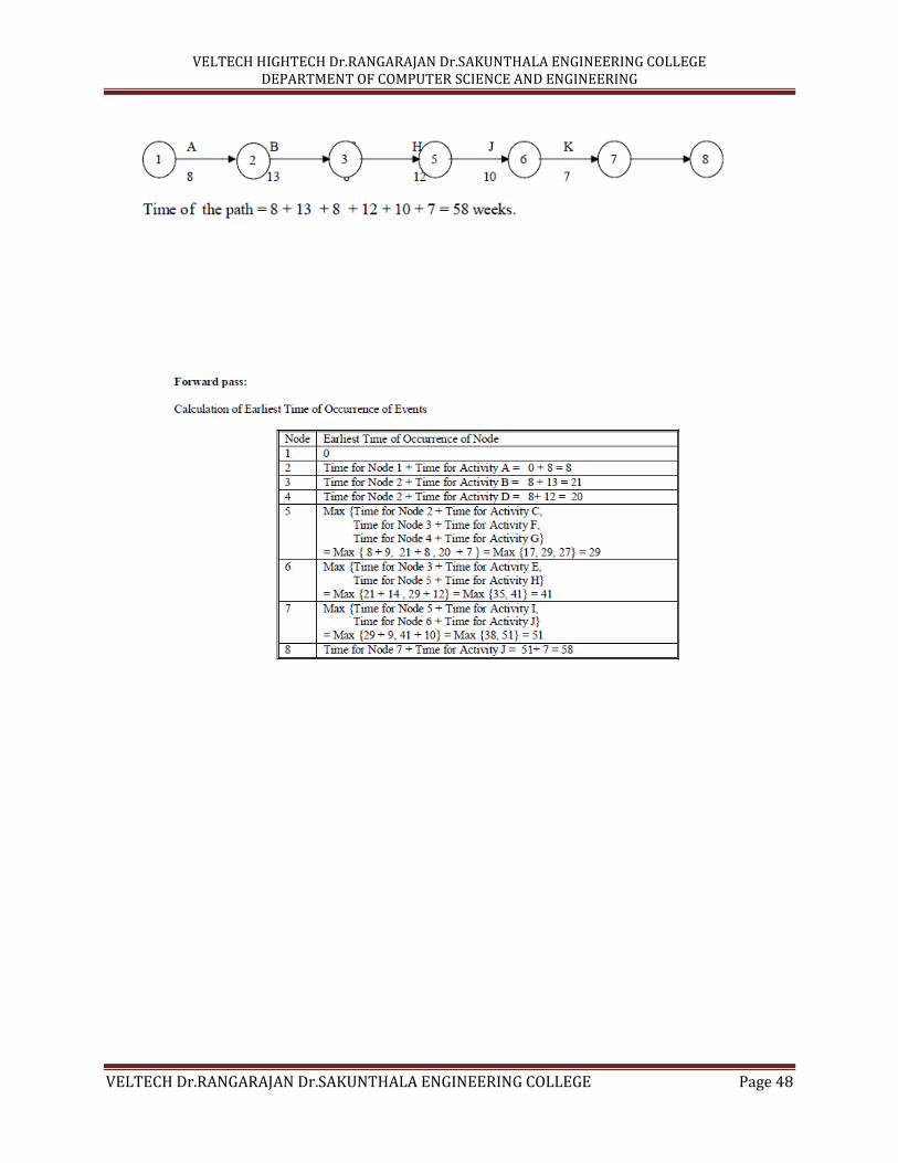
The longest path is the CPM , it is :
VELTECH HIGHTECH Dr.RANGARAJAN Dr.SAKUNTHALA ENGINEERING COLLEGE DEPARTMENT OF COMPUTER SCIENCE AND ENGINEERING
VELTECH Dr.RANGARAJAN Dr.SAKUNTHALA ENGINEERING COLLEGE Page 48

VELTECH HIGHTECH Dr.RANGARAJAN Dr.SAKUNTHALA ENGINEERING COLLEGE DEPARTMENT OF COMPUTER SCIENCE AND ENGINEERING
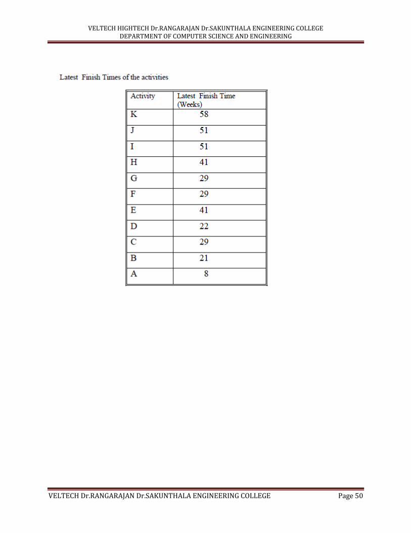
VELTECH Dr.RANGARAJAN Dr.SAKUNTHALA ENGINEERING COLLEGE Page 49
VELTECH HIGHTECH Dr.RANGARAJAN Dr.SAKUNTHALA ENGINEERING COLLEGE DEPARTMENT OF COMPUTER SCIENCE AND ENGINEERING
VELTECH Dr.RANGARAJAN Dr.SAKUNTHALA ENGINEERING COLLEGE Page 50

VELTECH HIGHTECH Dr.RANGARAJAN Dr.SAKUNTHALA ENGINEERING COLLEGE DEPARTMENT OF COMPUTER SCIENCE AND ENGINEERING
VELTECH Dr.RANGARAJAN Dr.SAKUNTHALA ENGINEERING COLLEGE Page 51
VELTECH HIGHTECH Dr.RANGARAJAN Dr.SAKUNTHALA ENGINEERING COLLEGE DEPARTMENT OF COMPUTER SCIENCE AND ENGINEERING
VELTECH Dr.RANGARAJAN Dr.SAKUNTHALA ENGINEERING COLLEGE Page 52
1. Find the expected duration and S.S of each activity.
2. Construct project net work.
3. Determine Critical path.
4. What is the probability that the project will be completed two
months later than expected .
We have already seen that in project shedule, we determine different
floats like free float, independent float and total float and use these
floats for resiources levelling and resource s allocation.
The procedure for Resource levelling is :
1. Draw the early start schedule graph.
2. Draw the corresponding manpower chart,
3. Identify the activities with slack.
4. Adjust the activities identified in 3 and adjust them to level the peak
resource requirement.
The procedure for Resource allocation program is :
1. Allocate resources serially in time .
2. If several jobs compete for the same resources give preference to the
jobs with the smallest slack.
3. Reshedule non critical jobs , if possible so as to make available tne
needed resources for resheduling critical jobs.
Reference: 1. Operations Research by Premkumar Gupta and D.S.HIRA, 2.
Resourcesmanagement techniques by Prof. Ssundaresan, K.S. Ganapathy
Subramaniam and K.Ganesan.
VELTECH HIGHTECH Dr.RANGARAJAN Dr.SAKUNTHALA ENGINEERING COLLEGE DEPARTMENT OF COMPUTER SCIENCE AND ENGINEERING
VELTECH Dr.RANGARAJAN Dr.SAKUNTHALA ENGINEERING COLLEGE Page 53
-
VELTECH HIGHTECH Dr.RANGARAJAN Dr.SAKUNTHALA ENGINEERING COLLEGE DEPARTMENT OF COMPUTER SCIENCE AND ENGINEERING
VELTECH Dr.RANGARAJAN Dr.SAKUNTHALA ENGINEERING COLLEGE Page 54


![Software Process - Undergraduate Coursescourses.cs.vt.edu/cs6704/spring17/slides/6704-2-SoftwareProcess.pdf · 1/18/17 2 Software Process • Definition [Pressman] – a framework](https://img.pdfslide.us/doc/110x75/5bd9906509d3f2e0688d5ce6/software-process-undergraduate-11817-2-software-process-definition-pressman.jpg)