Embed Size (px)
Citation preview
CS6302 DBMS IIYEARCSE
1
CS6302 - DATABASE MANAGEMENT SYSTEMS
1.1 INTRODUCTION
A database is a collection of data elements (facts) stored in a computer in a systematic
way, such that a computer program can consult it to answer questions. The answers to those
questions become information that can be used to make decisions that may not be made with the
data elements alone. The computer program used to manage and query a database is known as a
database management system (DBMS). So a database is a collection of related data that we can use for
Defining - specifying types of data
Constructing - storing & populating
Manipulating - querying, updating, reporting
A Database Management System (DBMS) is a software package to facilitate the creation
and maintenance of a computerized database. A Database System (DBS) is a DBMS together
with the data itself. 1.1.1 Features of a database:
It is a persistent (stored) collection of related data. The data is input (stored) only once. The data is organised (in some fashion). The data is accessible and can be queried (effectively and efficiently). 1.1.2 File systems vs Database systems:
DBMS are expensive to create in terms of software, hardware, and time invested. So why
use them? Why couldn‘t we just keep all our data in files, and use word-processors to edit the
files appropriately to insert, delete, or update data? And we could write our own programs to
query the data! This solution is called maintaining data in flat files. So what is bad about flat
files?
Uncontrolled redundancy
Inconsistent data Inflexibility Limited data sharing
CS6302 DBMS IIYEARCSE
2
Poor enforcement of standards Low programmer productivity Excessive program maintenance
Excessive data maintenance
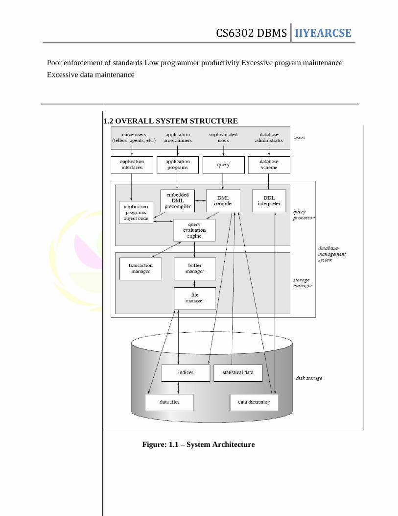
1.2 OVERALL SYSTEM STRUCTURE
Figure: 1.1 – System Architecture
CS6302 DBMS IIYEARCSE
3
1.1.3 Drawbacks of using file systems to store data: Data redundancy and inconsistency Due to availability of multiple file formats, storage in files may cause duplication of information
in different files.
Difficulty in accessing data In order to retrieve, access and use stored data, need to write a new program to carry out each
new task.
Data isolation To isolate data we need to store them in multiple files and different formats. Integrity problems Integrity constraints (E.g. account balance > 0) become part of program code which has to be
written every time. It is hard to add new constraints or to change existing ones. Atomicity of updates Failures of files may leave database in an inconsistent state with partial updates carried out.
E.g. transfer of funds from one account to another should either complete or not happen at all
CS6302 DBMS IIYEARCSE
4
The Overall structure of the database system is shown in Figure 1.1. The Central
component is known as the core DBMS which has a query evaluation engine to execute the
queries. The disk storage is used to store the data.
1.2 Database Users:
Users are differentiated by the way they expect to interact with the system Application
programmers – interact with the system through DML calls
Specialized users – write specialized database applications that do not fit into the traditional data processing framework
Naive users – invoke one of the permanent application programs that have been written
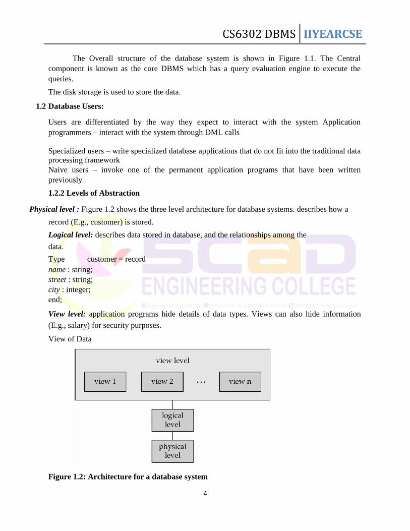
previously 1.2.2 Levels of Abstraction
Physical level : Figure 1.2 shows the three level architecture for database systems. describes how a
record (E.g., customer) is stored. Logical level: describes data stored in database, and the relationships among the data. Type customer = record name : string; street : string; city : integer; end; View level: application programs hide details of data types. Views can also hide information
(E.g., salary) for security purposes. View of Data Figure 1.2: Architecture for a database system
CS6302 DBMS IIYEARCSE
5
1.2.3 Instances and Schemas
Similar to types and variables in programming languages which we already know,
Schema is the logical structure of the database E.g., the database consists of information about a
set of customers and accounts and the relationship between them) analogous to type information
of a variable in a program. Physical schema: database design at the physical level
Logical schema: database design at the logical level
Instance is the actual content of the database at a particular point of time, analogous to
the value of a variable.
Physical Data Independence – the ability to modify the physical schema without
changing the logical schema. Applications depend on the logical schema.
In general, the interfaces between the various levels and components should be well
defined so that changes in some parts do not seriously influence others.
1.3 DATA MODELS
o A structure that demonstrates all the required features of the parts of
the real world, which is of interest to the users of the information in the
model.
o Representation and reflection of the real world (Universe of Discourse).
o A set of concepts that can be used to describe the structure of a
database: the data types, relationships, constraints, semantics and
operational behaviour.
o It is a tool for data abstraction
o A collection of tools for describing
data
data relationships
data semantics
data constraints Some of the data models are : o Entity-Relationship model o Relational model
CS6302 DBMS IIYEARCSE
6
o Other models:
object-oriented model semi-structured data models Older models: network model and hierarchical model
A data model is described by the schema, which is held in the data dictionary.
Student(studno,name,address) Course(courseno,lecturer) Schema
Student(123,Bloggs,Woolton) Instance
(321,Jones,Owens)
Example: Consider the database of a bank and its accounts, given in Table 1.1
and Table 1.2
Table 1.1. ―Account‖ contains details
of Table 1.2. ―Customer‖ contains details of
the customer of a
bank the bank account
Customer
Account
Account Balance
Name Area City
Number
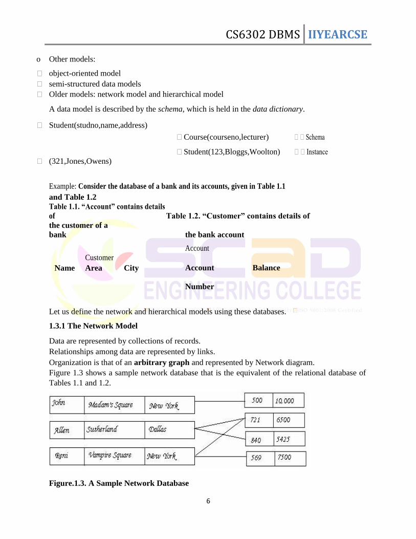
Let us define the network and hierarchical models using these databases. 1.3.1 The Network Model Data are represented by collections of records. Relationships among data are represented by links. Organization is that of an arbitrary graph and represented by Network diagram. Figure 1.3 shows a sample network database that is the equivalent of the relational database of
Tables 1.1 and 1.2.
Figure.1.3. A Sample Network Database
CS6302 DBMS IIYEARCSE
7
The CODASYL/DBTG database was derived on this model. Constraints in the Network Model:
1. Insertion Constraints: Specifies what should happen when a record is inserted.
2. Retention Constraints: Specifies whether a record must exist on its own or always be related to
an owner as a member of some set instance.
3. Set Ordering Constraints: Specifies how a record is ordered inside the database.
4. Set Selection Constraints: Specifies how a record can be selected from the database.
1.3.2 The Hierarchical Model Similar to the network model and the concepts are derived from the earlier systems Information
Management System and System-200.
Organization of the records is as a collection of trees, rather than arbitrary
graphs.
In the hierarchical model, a Schema represented by a Hierarchical Diagram as
shown in Figure 1.4 in which
o One record type, called Root, does not participate as a child record
type.
o Every record type except the root participates as a child record type in
exactly one type.
o Leaf is a record that does not participate in any record types.
o A record can act as a Parent for any number of records.
Figure.1.4. A Sample Hierarchical Database
The relational model does not use pointers or links, but relates records by the values they
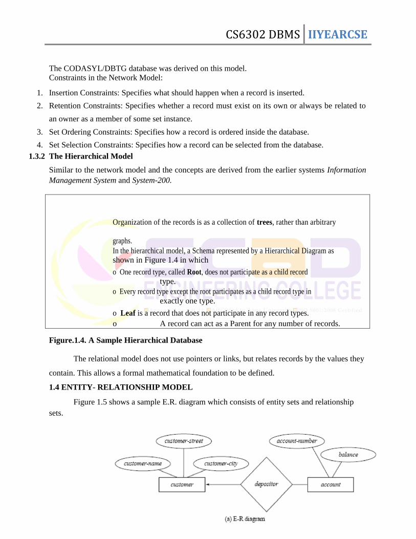
contain. This allows a formal mathematical foundation to be defined. 1.4 ENTITY- RELATIONSHIP MODEL
Figure 1.5 shows a sample E.R. diagram which consists of entity sets and relationship
sets.
CS6302 DBMS IIYEARCSE
8
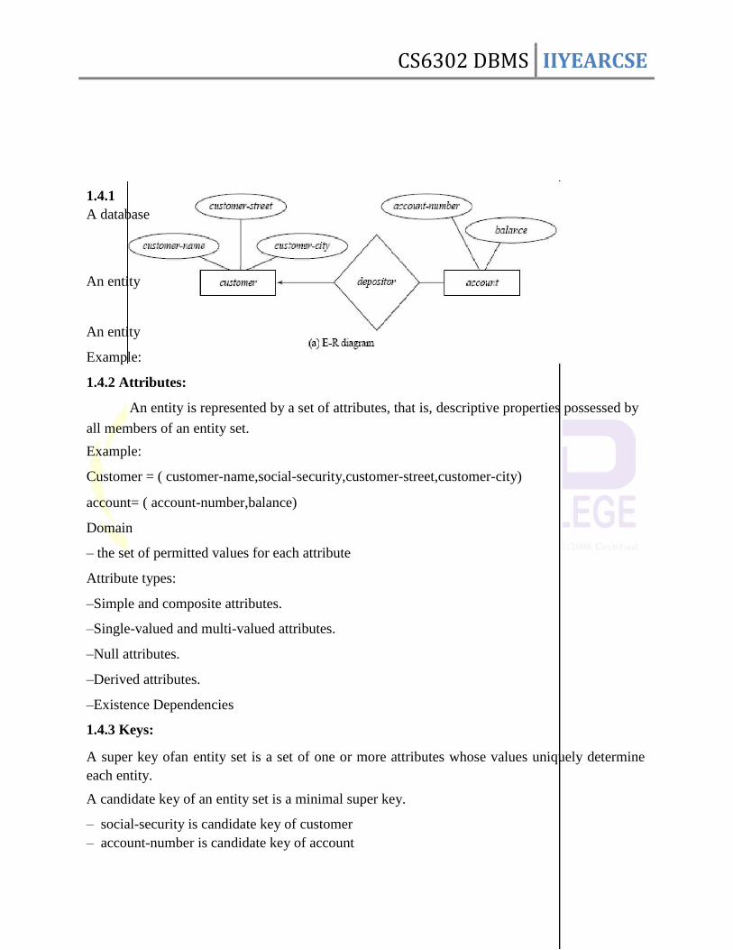
1.4.1
A database An entity
An entity Example: 1.4.2 Attributes:
An entity is represented by a set of attributes, that is, descriptive properties possessed by
all members of an entity set. Example: Customer = ( customer-name,social-security,customer-street,customer-city) account= ( account-number,balance) Domain – the set of permitted values for each attribute Attribute types: –Simple and composite attributes. –Single-valued and multi-valued attributes. –Null attributes. –Derived attributes. –Existence Dependencies 1.4.3 Keys:
A super key ofan entity set is a set of one or more attributes whose values uniquely determine
each entity. A candidate key of an entity set is a minimal super key. – social-security is candidate key of customer – account-number is candidate key of account
CS6302 DBMS IIYEARCSE
9
Although several candidate keys may exist, one of the candidate keys is selected to be the
primary key.
CS6302 DBMS IIYEARCSE
10
1.4.4 E-R Diagram Components
Rectangles represent entity sets. Ellipses represent attributes. Diamonds represent relationship sets.
Lines link attributes to entity sets and entity sets to relationship sets. Double ellipses represent
multivalued attributes.
Dashed ellipses denote derived attributes. Primary key attributes are underlined.
1.4.5 Weak Entity Set
An entity set that does not have a primary key is referred to as a weak entity set. The
existence of a weak entity set depends on the existence of a strong entity set; it must relate to the
strong set via a one-to-many relationship set. The discriminator (or partial key) of a weak entity
set is the set of attributes that distinguishes among all the entities of a weak entity set. The
primary key of a weak entity set is formed by the primary key of the strong entity set on which
the weak entity set is existence dependent, plus the weak entity set‘s discriminator. A weak entity
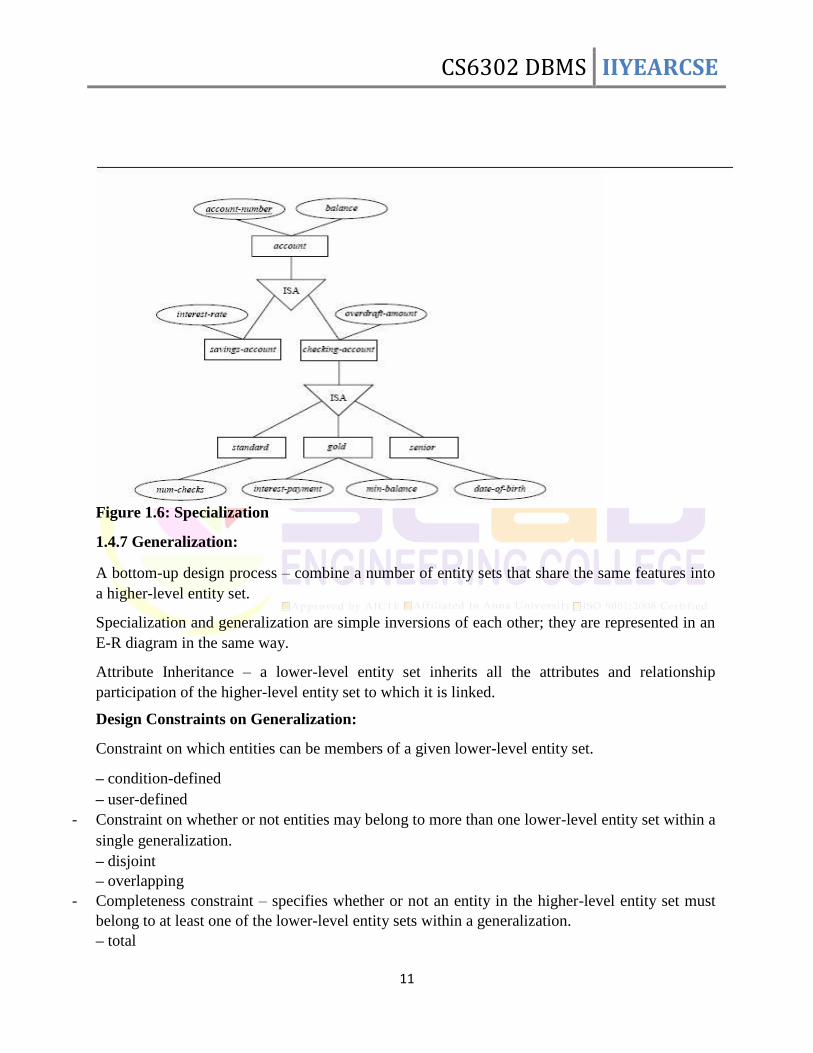
set is depicted by double rectangles. 1.4.6 Specialization
This is a Top-down design process as whown in Figure 1.6 in which; we designate
subgroupings within an entity set that are distinctive from other entitie in the set.
These subgroupings become lower-level entity sets that have attributes or participate in
relationships that do not apply to the higher-level entity set.
Depicted by a triangle component labeled ISA (i.e., savings-account ―is an‖ account)
CS6302 DBMS IIYEARCSE
11
Figure 1.6: Specialization 1.4.7 Generalization:
A bottom-up design process – combine a number of entity sets that share the same features into
a higher-level entity set. Specialization and generalization are simple inversions of each other; they are represented in an
E-R diagram in the same way. Attribute Inheritance – a lower-level entity set inherits all the attributes and relationship
participation of the higher-level entity set to which it is linked. Design Constraints on Generalization: Constraint on which entities can be members of a given lower-level entity set. – condition-defined – user-defined
- Constraint on whether or not entities may belong to more than one lower-level entity set within a
single generalization.
– disjoint – overlapping
- Completeness constraint – specifies whether or not an entity in the higher-level entity set must
belong to at least one of the lower-level entity sets within a generalization.
– total
CS6302 DBMS IIYEARCSE
12
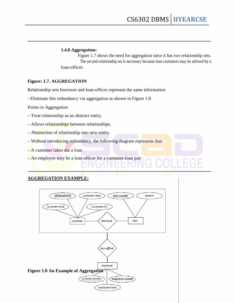
1.4.8 Aggregation:
Figure 1.7 shows the need for aggregation since it has two relationship sets.
The second relationship set is necessary because loan customers may be advised by a
loan-officer. Figure: 1.7. AGGREGATION Relationship sets borrower and loan-officer represent the same information - Eliminate this redundancy via aggregation as shown in Figure 1.8 Points in Aggregation – Treat relationship as an abstract entity. – Allows relationships between relationships. – Abstraction of relationship into new entity. – Without introducing redundancy, the following diagram represents that: – A customer takes out a loan – An employee may be a loan officer for a customer-loan pair
AGGREGATION EXAMPLE:
Figure 1.8 An Example of Aggregation
CS6302 DBMS IIYEARCSE
13
RELATIONAL ALGEBRA
Procedural language Six basic operators are fundamental in relational algebra Theyare o select o project o union o set difference o Cartesian product o rename
The operators take two or more relations as inputs and give a new relation as a result.
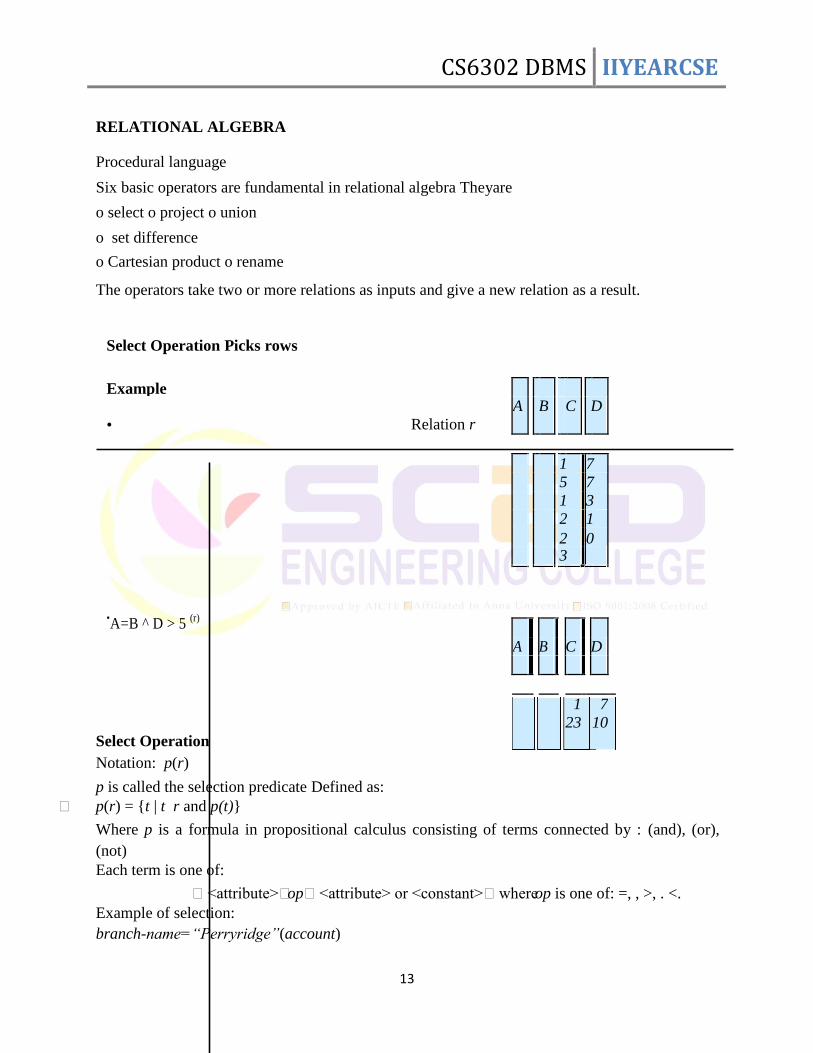
Select Operation Picks rows
Example
A
B
C
D
• Relation r
1 7
5 7
1 3
2 1
2 0
3
•A=B ^ D > 5
(r)
A
B
C
D
1 7
23 10
Select Operation Notation: p(r) p is called the selection predicate Defined as:
p(r) = {t | t r and p(t)} Where p is a formula in propositional calculus consisting of terms connected by : (and), (or),
(not) Each term is one of:
<attribute>op<attribute> or <constant>where op is one of: =, , >, . <. Example of selection: branch-name=―Perryridge‖(account)
CS6302 DBMS IIYEARCSE
14
Example of selection:
Project Operation Notation: A1, A2, …, Ak (r) where A1, A2 are attribute names and r is a relation name.
The result is defined as the relation of k columns obtained by erasing the columns that are not
listed
Duplicate rows removed from result, since relations are sets E.g. To eliminate the branch-name
attribute of account account-number, balance (account) Union Operation
Notation: r s Defined as:
r s = {t | t r or t s} For r s to be valid,
r, s must have the same arity (same number of attributes) The attribute
domains must be compatible (E.g., 2nd column
of r deals with the same type of values as does the 2nd column of s) E.g. to find all customers with either an account or a loan customer-name (depositor) customer-name (borrower)
Notation r – s
Defined as:
r – s = {t | t r and t s}
Set differences must be taken between compatible relations. o r and s must have the same arity o attribute domains of r and s must be compatible
Cartesian-Product Operation-Example Cartesian-Product Operation
Notation r x s
Defined as:
r x s = {t q | t r and q s}
CS6302 DBMS IIYEARCSE
15
R S = ).
If attributes of r(R) and s(S) are not disjoint, then renaming must be used.
Composition of Operations
Can build expressions using multiple operations Example: A=C(r x s)
Rename Operation
Allows us to name, and therefore to refer to, the results of relational-algebra expressions.
Allows us to refer to a relation by more than one name. Example: x (E) returns the expression E under the name X If a relational-algebra expression E has arity n, then x (A1, A2, …, An) (E) returns the result of expression E under the name X, and with the attributes renamed to A1, A2,
…., An. 2.3.8 Banking Example branch (branch-name, branch-city, assets) customer (customer-name, customer-street, customer-only) account (account-number, branch-
name, balance) loan (loan-number, branch-name, amount) depositor (customer-name, account-numbe)
borrower (customer-name, loan-number)
CS6302 DBMS IIYEARCSE
16
Formal Definition of Relational Algebra A basic expression in the relational algebra consists of either one of the following: o A relation in the database o A constant relation Let E1 and E2 be relational-algebra expressions; the following are all relational-algebra
expressions:
o E1 E2 o E1 - E2 o E1 x E2 o p (E1), P is a predicate on attributes in E1 o s(E1), S is a list consisting of some of the attributes in E1 o x (E1), x is the new name for the result of E1
Modification of the Database
The content of the database may be modified using the following operations: o Deletion
o Insertion o Updating
All these operations are expressed using the assignment operator. Deletion
A delete request is expressed similarly to a query, except instead of displaying tuples to the user,
the selected tuples are removed from the database. Can delete only whole tuples; cannot delete values on only particular attributes.
Examples
Delete all account records in the Perryridge branch.
account account – branch-name = ―Perryridge‖ (account)
Delete all loan records with amount in the range of 0 to 50 loan loan
– amount 0 and amount 50
(loan)
Delete all accounts at branches located in Needham.
r1 branch-city = ―Needham‖ (account branch)
r2 (r1)
branch-name, account-number, balance
r
3 customer-name, account-number (r2 depositor)
account account – r2 depositor depositor – r3 Insertion
To insert data into a relation, we either: o specify a tuple to be inserted.
o write a query whose result is a set of tuples to be inserted. in relational algebra, an insertion
is expressed by:
CS6302 DBMS IIYEARCSE
17
r r E where r is a relation and E is a relational algebra expression.
The insertion of a single tuple is expressed by letting E be a constant relation containing one
tuple. Examples Insert information in the database specifying that Smith has $1200 in account A-973 at the Perryridge branch. account account {(―Perryridge‖, A-973, 1200)} depositor depositor {(―Smith‖, A-973)} Provide as a gift for all loan customers in the Perryridge branch, a $200 savings account. Let the
loan number serve as the account number for the new savings account. r1
( branch-name = ―Perryridge‖
(borrower loan)) account account branch-name, account-number,200 (r1) depositor
Updating:
A mechanism to change a value in a tuple without changing all values in the tuple. Use the generalized projection operator to do this task
r F1, F2, …, FI, (r) Each Fi is either o the ith attribute of r, if the ith attribute is not updated, or,
o if the attribute is to be updated Fi is an expression, involving only constants and the attributes of
r, which gives the new value for the attribute. Examples Make interest payments by increasing all balances by 5 percent. account AN, BN, BAL * 1.05 (account) where AN, BN and BAL stand for account-number, branch-name and balance, respectively. Pay all accounts with balances over $10,000 6 percent interest and pay all others 5 percent
account AN, BN, BAL * 1.06
( BAL 10000
(account))
AN, BN, BAL * 1.05 ( BAL 10000
(account))
Functional Dependencies Definition Functional dependency (FD) is a constraint between two sets attributes from the database. A functional dependency is a property of the semantics or meaning of the attributes. In every relation R(A1, A2,…, An) there is a FD called the PK -> A1, A2, …, An Formally the FD is defined as follows If X and Y are two sets of attributes, that are subsets of T For any two tuples t1 and t2 in r , if t1[X]=t2[X], we must also have t1[Y]=t2[Y].
CS6302 DBMS IIYEARCSE
18
Notation: o If the values of Y are determined by the values of X, then it is denoted by X -> Y
o Given the value of one attribute, we can determine the value of another attribute
X f.d. Y or X -> y Example: Consider the following, Student Number -> Address, Faculty Number -> Department, Department Code -> Head of Dept Goal — Devise a Theory for the Following Decide whether a particular relation R is in ―good‖ form.
In the case that a relation R is not in ―good‖ form, decompose it into a set of relations {R1, R2, ...,
Rn} such that o each relation is in good form.
o the decomposition is a lossless-join decomposition. Our
theory is based on: o functional dependencies
o multivalued dependencies
2.8.1 Functional Dependencies
o Constraints on the set of legal relations.
o Require that the value for a certain set of attributes determines uniquely the value for another set
of attributes. o A functional dependency is a generalization of the notion of a key.
o The functional dependency α holds on R if and only if for any legal relations r(R), whenever any two tuples t1 and t2 of r agree
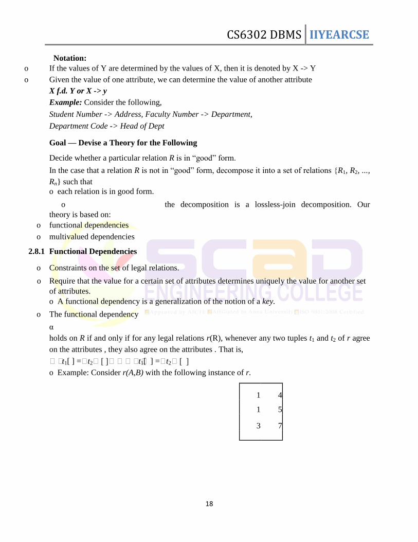
on the attributes , they also agree on the attributes . That is, t1[ ] =t2[ ]t1[ ] =t2[ ] o Example: Consider r(A,B) with the following instance of r.
1 4
1 5
3 7
CS6302 DBMS IIYEARCSE
19
o On this instance, A B does NOT hold, but B A does hold.
K is a superkey for relation schema R if and only if K R K is a candidate key for R if and only if o K R, and o for no K, R Functional dependencies allow us to express constraints that cannot be expressed using
superkeys. Consider the schema: Loan-info-schema = (customer-name, loan-number, branch-name, amount). We expect this set of functional dependencies to hold: loan-number amount
loan-number branch-name but would not expect the following to hold: loan-number customer-name 2.8.2 Use of Functional Dependencies We use functional dependencies to:
o test relations to see if they are legal under a given set of functional dependencies. o If a relation r is legal under a set F of functional dependencies, we say that r satisfies F.
o specify constraints on the set of legal relations
o We say that F holds on R if all legal relations on R satisfy the set of functional dependencies F. Note: A specific instance of a relation schema may satisfy a functional dependency even if the
functional dependency does not hold on all legal instances. o For example, a specific instance of Loan-schema may, by chance, satisfy loan-number
customer-name. A functional dependency is trivial if it is satisfied by all instances of a relation. E.g.
o customer-name, loan-number customer-name o customer-name customer-name
o In general, is trivial if 2.8.3 Closure of a Set of Functional Dependencies
Given a set F set of functional dependencies, there are certain other functional dependencies that
are logically implied by F. o E.g. If A B and B C, then we can infer that A C
CS6302 DBMS IIYEARCSE
20
The set of all functional dependencies logically implied by F is the closure of F.
We denote the closure of F by F+.
We can find all of F+ by applying Armstrong‘s Axioms:
o if, then (reflexivity)
o if, then (augmentation)
o if, and, then(transitivity) These rules are o sound (generate only functional dependencies that actually hold) and o complete (generate all
functional dependencies that hold).
Example R = (A, B, C, G, H, I) F = { A B A C CG H CG I B H} NORMALIZATION – NORMAL FORMS
o Introduced by Codd in 1972 as a way to ―certify‖ that a relation has a certain level of
normalization by using a series of tests. o It is a top-down approach, so it is considered relational design by analysis. o It is based on the
rule: one fact – one place.
o It is the process of ensuring that a schema design is free of redundancy. 2.9.1 Uses of Normalization o Minimize redundancy o Minimize update anomalies o We use normal form tests to determine the level of normalization for the scheme. Pitfalls in Relational Database Design
Relational database design requires that we find a ―good‖ collection of relation schemas. A bad
design may lead to o Repetition of Information. o Inability to represent certain information. Design Goals: o Avoid redundant data. o Ensure that relationships among attributes are represented o Facilitate the checking of updates
for violation of database integrity constraints.
CS6302 DBMS IIYEARCSE
21
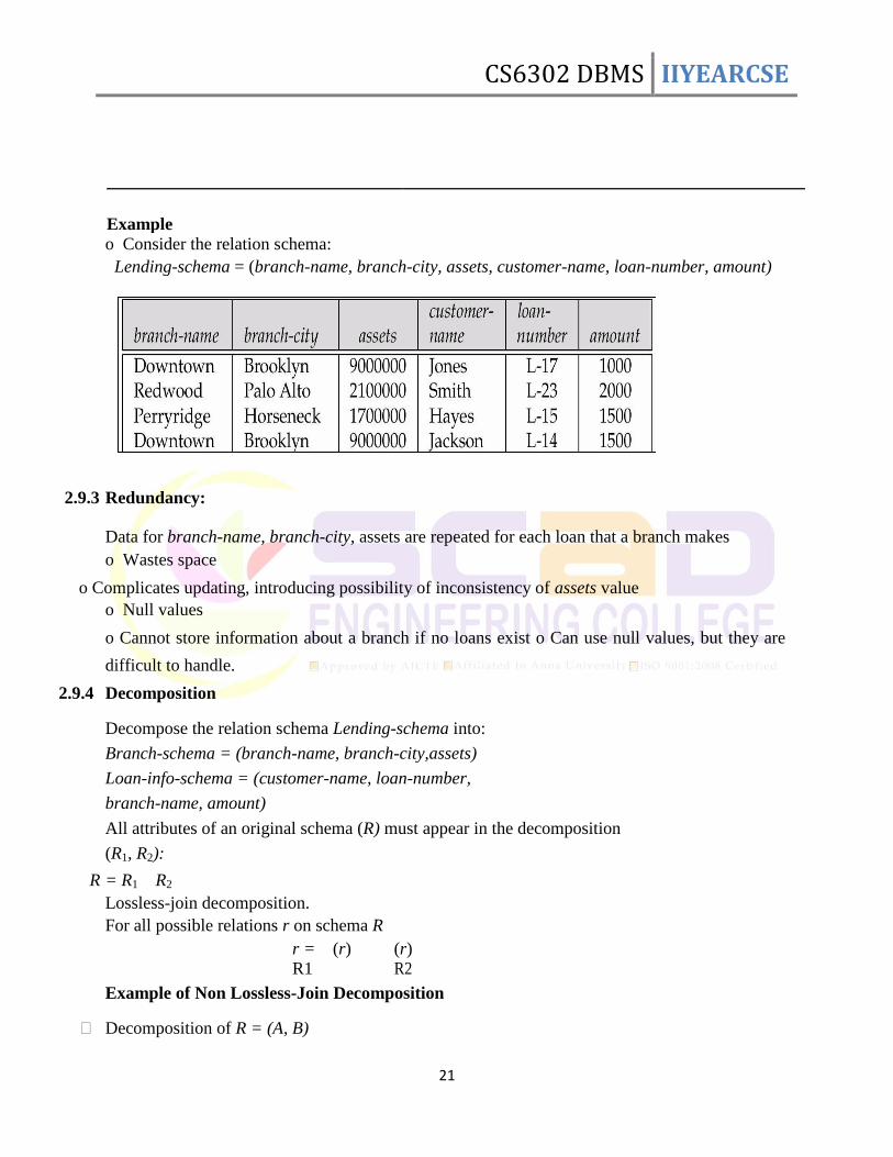
Example
o Consider the relation schema: Lending-schema = (branch-name, branch-city, assets, customer-name, loan-number, amount)
2.9.3 Redundancy:
Data for branch-name, branch-city, assets are repeated for each loan that a branch makes o Wastes space
o Complicates updating, introducing possibility of inconsistency of assets value o Null values o Cannot store information about a branch if no loans exist o Can use null values, but they are
difficult to handle.
2.9.4 Decomposition Decompose the relation schema Lending-schema into: Branch-schema = (branch-name, branch-city,assets) Loan-info-schema = (customer-name, loan-number, branch-name, amount) All attributes of an original schema (R) must appear in the decomposition (R1, R2):
R = R1 R2 Lossless-join decomposition. For all possible relations r on schema R
r = (r) (r) R1 R2
Example of Non Lossless-Join Decomposition
Decomposition of R = (A, B)
CS6302 DBMS IIYEARCSE
22
R2 = (A) R2 = (B)
Normalization Using Functional Dependencies
When we decompose a relation schema R with a set of functional dependencies F into R1, R2,.., Rn we want Lossless-join decomposition: Otherwise decomposition would result
in information loss. No redundancy: The relations Ri preferably should be in either Boyce-Codd Normal Form or
Third Normal Form. Dependency preservation: Let Fi be the set of dependencies F
+ that include only attributes in Ri.
o Preferably the decomposition should be dependency preserving,
that is, (F F … F )+ = F
+
12 n Otherwise, checking updates for violation of functional dependencies may require computing
joins, which is expensive. Example
R = (A, B, C) F = {A B, B C)
Can be decomposed in two different ways. o R1 = (A, B), R2 = (B, C)
Lossless-join decomposition: o R1 R2 = {B} and B BC
Dependency preserving.
o R1 = (A, B), R2 = (A, C) Lossless-join decomposition:
o R1 R2 = {A} and A AB
Testing preservation:
To check if a dependency is preserved in a decomposition of R into R1, R2, …, Rn we apply the following simplified test (with attribute closure done with reference.
F)
result = while (changes to result) do
for each Ri in the decomposition t = (result Ri)+ Ri result = result t
If result contains all attributes in , then the functional dependency is preserved. We apply the test on all dependencies in F to check if a decomposition is dependency preserving
This procedure takes polynomial time, instead of the exponential time required to compute F+
and (F1 F2 … Fn)+
CS6302 DBMS IIYEARCSE
23
1NF 2NF 3NF
Boyce-Codd NF 4NF 5NF
2.10 TYPES OF NORMAL FORMS 2.10.1 First Normal Form (1NF) o Now part of the formal definition of a relation. o Attributes may only have atomic values (i.e. single values). o Disallows ―relations within relations‖ or ―relations as attributes of tuples‖. 2.10.2 Second Normal Form (2NF)
o A relation is in 2NF if all of its non-key attributes are fully dependent on the key.
o This is known as full functional dependency. o When in 2NF, the removal of any attribute will break the dependency
R (fnum, dcode, fname, frank, dname) R1(fnum, fname, frank)
R2(dcode, dname)
2.10.3 Third Normal Form (3NF)
o A relation is in 3NF if it is in 2NF and has no transitive dependencies
o A transitive dependency is when X->Y and Y->Z implies X->Z Faculty (number, fname, frank, dname, doffice, dphone) R1 (number, fname, frank, dname)
R2 (dname, doffice, dphone) R (snum, cnum, dcode, s_term, s_slot, fnum, c_title, c_description, f_rank, f_name, d_name,
d_phones) The following is the 3NF of above schema,
1. snum, cnum, dcode -> s_term, s_slot, fnum, c_title, c_description, f_rank, f_name, d_name,
d_phones
CS6302 DBMS IIYEARCSE
24
2. dcode -> d_name 3. cnum, dcode -> c_title, c_description 4. cnum, dcode, snum -> s_term, s_slot, fnum, f_rank, f_name 5. fnum -> f_rank, f_name
Boyce Codd Normal Form (BCNF)
o It is based on FD that takes into account all candidate keys in a relation. o A relation is said to
be in BCNF if and only if every determinant is a candidate key.
o A determinant is an attribute or a group of attributes on which some other attribute is fully
functionally determinant o To test whether a relation is in BCNF, we identify all the determinants and make sure that they are
candidate keys.
UNIT II
SQL & QUERY OPTIMIZATION
2.4 STRUCTURED QUERY LANGUAGE (SQL) 2.4.1 Introduction
Structured Query Language (SQL) is a data sub language that has constructs for defining and
processing a database. It can be H Used stand-alone within a DBMS command H Embedded in triggers and stored procedures H Used in scripting or programming languages History of SQL-92
SQL was developed by IBM in late 1970s.
SQL-92 was endorsed as a national standard by ANSI in 1992.
SQL3 incorporates some object-oriented concepts but has not gained acceptance in industry.
CS6302 DBMS IIYEARCSE
25
Data Manipulation Language (DML) is used to query and update data. Each SQL statement is terminated with a semicolon.
2.4.2. Create Table
CREATE TABLE statement is used for creating relations. Each column is described with three parts: column name, data type, and optional constraints. Example: CREATE TABLE PROJECT (ProjectID Integer Primary Key, Name Char(25) Unique Not Null,
Department VarChar (100) Null, MaxHours Numeric(6,1) Default 100); Data Types Standard data types – Char for fixed-length character
– VarChar for variable-length character, It requires additional processing than Char data types
– Integer for whole number – Numeric Constraints
Constraints can be defined within the CREATE TABLE statement, or they can be added to the
table after it is created using the ALTER table statement. Five types of constraints: H PRIMARY KEY may not have null values H UNIQUE may have null values H NULL/NOT NULL H FOREIGN KEY
H CHECK
2.4.3 ALTER Statement
ALTER statement changes table structure, properties, or constraints after it has been created. Example ALTER TABLE ASSIGNMENT ADD CONSTRAINT EmployeeFK FOREIGN KEY (EmployeeNum) REFERENCES EMPLOYEE (EmployeeNumber) ON UPDATE CASCADE ON DELETE NO ACTION;
CS6302 DBMS IIYEARCSE
26
2.4.4 DROP Statements DROP TABLE statement removes tables and their data from the database
A table cannot be dropped if it contains foreign key values needed by other tables. H Use ALTER
TABLE DROP CONSTRAINT to remove integrity constraints
in the other table first Example: H DROP TABLE CUSTOMER; H ALTER TABLE ASSIGNMENT DROP CONSTRAINT ProjectFK;
2.4.5 SELECT Statement
SELECT can be used to obtain values of specific columns, specific rows, or both. Basic format: SELECT (column names or *) FROM (table name(s)) [WHERE (conditions)]; WHERE Clause Conditions
Require quotes around values for Char and VarChar columns, but no quotes for Integer and
Numeric columns. AND may be used for compound conditions. IN and NOT IN indicate ‗match any‘ and ‗match all‘ sets of values, respectively. Wildcards _
and % can be used with LIKE to specify a single or multiple unknown characters, respectively. IS NULL can be used to test for null values. Example: SELECT Statement SELECT Name, Department, MaxHours FROM PROJECT;WHERE Name=‖XYX‖; Sorting the Results ORDER BY phrase can be used to sort rows from SELECT statement. SELECT Name, Department FROM EMPLOYEE ORDER BY Department;
Two or more columns may be used for sorting purposes. SELECT Name, Department FROM EMPLOYEE ORDER BY Department DESC, Name ASC;
CS6302 DBMS IIYEARCSE
27
INSERT INTO Statement The order of the column names must match the order of the values. Values for all NOT NULL
columns must be provided. No value needs to be provided for a surrogate primary key. It is possible to use a select statement to provide the values for bulk inserts from a second table. Examples:
– INSERT INTO PROJECT VALUES (1600, ‗Q4 Tax Prep‘, ‗Accounting‘, 100);
– INSERT INTO PROJECT (Name, ProjectID) VALUES (‗Q1+ Tax Prep‘, 1700); UPDATE Statement
UPDATE statement is used to modify values of existing data. Example: UPDATE EMPLOYEE SET Phone = ‘287-1435’ WHERE Name = ‘James’; UPDATE can also be used to modify more than one column value at a time UPDATE EMPLOYEE SET Phone = ‘285-0091’, Department = ‘Production’ WHERE EmployeeNumber = 200; DELETE FROM Statement
Delete statement eliminates rows from a table. Example DELETE FROM PROJECT WHERE Department = ‗Accounting‘; ON DELETE CASCADE removes any related referential integrity constraint Basic Queries Using Single Row Functions Date Functions months_between(date1, date2)
1. select empno, ename, months_between (sysdate, hiredate)/12 from emp;
2. select empno, ename, round((months_between(sysdate, hiredate)/ 12), 0) from emp;
3. select empno, ename, trunc((months_between(sysdate, hiredate)/12), 0) from emp;
1. select ename, add_months (hiredate, 48) from emp; 2. select ename, hiredate, add_months (hiredate, 48) from emp;
last_day(date)
1. select hiredate, last_day(hiredate) from emp; next_day(date, day)
1. select hiredate, next_day(hiredate, ‗MONDAY‘) from emp;
CS6302 DBMS IIYEARCSE
28
Trunc(date, [Foramt])
1. select hiredate, trunc(hiredate, ‗MON‘) from emp;
2. select hiredate, trunc(hiredate, ‗YEAR‘) from emp; Character Based Functions initcap(char_column)
1. select initcap(ename), ename from emp; lower(char_column)
1. select lower(ename) from emp; Ltrim(char_column, ‗STRING‘)
1. select ltrim(ename, ‗J‘) from emp; Ltrim(char_column, ‗STRING‘)
1. select rtrim(ename, ‗ER‘) from emp; Translate(char_column, ‗search char,‗replacement char)
1. select ename, translate(ename, ‗J‘, ‗CL‘) from emp; replace(char_column, ‗search string‘,‗replacement string‘)
1. select ename, replace(ename, ‗J‘, ‗CL‘) from emp; Substr(char_column, start_loc, total_char)
1. select ename, substr(ename, 3, 4) from emp; Mathematical Functions Abs(numerical_column)
1. select abs(-123) from dual; ceil(numerical_column)
1. select ceil(123.0452) from dual; floor(numerical_column)
1. select floor(12.3625) from dual; Power(m,n)
1. select power(2,4) from dual;
CS6302 DBMS IIYEARCSE
29
Mod(m,n)
1. select mod(10,2) from dual;
Round(num_col, size)
1. select round(123.26516, 3) from dual;
Trunc(num_col,size)
1. select trunc(123.26516, 3) from dual;
sqrt(num_column)
1. select sqrt(100) from dual; Complex Queries Using Group Function
Group Functions There are five built-in functions for SELECT statement:
1. COUNT counts the number of rows in the result
2. SUM totals the values in a numeric column 3. AVG calculates an average value 4. MAX retrieves a maximum value 5. MIN retrieves a minimum value
Result is a single number (relation with a single row and a single column). Column names
cannot be mixed with built-in functions. Built-in functions cannot be used in WHERE clauses. Example: Built-in Functions
1. Select count (distinct department) from project; 2. Select min (maxhours), max (maxhours), sum (maxhours) from project;
3. Select Avg(sal) from emp;
Built-in Functions and Grouping GROUP BY allows a column and a built-in function to be used together. GROUP BY sorts the table by the named column and applies the built-in function to groups of
rows having the same value of the named column. WHERE condition must be applied before GROUP BY phrase. Example
Select department, count (*) from employee where employee_number < 600 group by department having count (*) > 1;
CS6302 DBMS IIYEARCSE
30
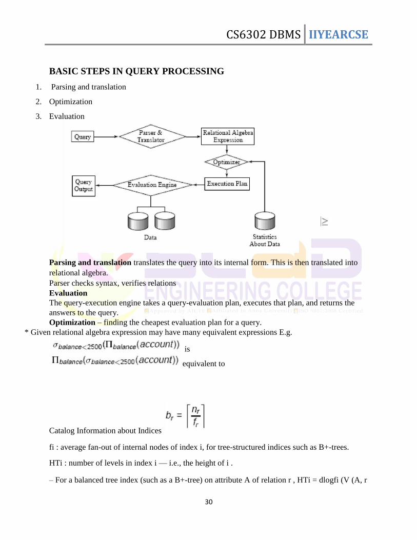
BASIC STEPS IN QUERY PROCESSING
1. Parsing and translation
2. Optimization
3. Evaluation
Parsing and translation translates the query into its internal form. This is then translated into
relational algebra. Parser checks syntax, verifies relations Evaluation The query-execution engine takes a query-evaluation plan, executes that plan, and returns the
answers to the query. Optimization – finding the cheapest evaluation plan for a query.
* Given relational algebra expression may have many equivalent expressions E.g.
is
equivalent to
Catalog Information about Indices fi : average fan-out of internal nodes of index i, for tree-structured indices such as B+-trees. HTi : number of levels in index i — i.e., the height of i . – For a balanced tree index (such as a B+-tree) on attribute A of relation r , HTi = dlogfi (V (A, r
CS6302 DBMS IIYEARCSE
31
)e. – For a hash index, HTi is 1. LBi : number of lowest-level index blocks in i — i.e., the number of blocks at the leaf level of
the index. Measures of Query Cost
• Many possible ways to estimate cost, for instance disk accesses, CPU time, or even
communication overhead in a distributed or parallel system.
Typically disk access is the predominant cost, and is also relatively easy to
estimate. Therefore number of block transfers from disk is used as a measure
of the actual cost of evaluation. It is assumed that all transfers of blocks have
the same cost.
• Costs of algorithms depend on the size of the buffer in main memory, as having more memory
reduces need for disk access. Thus memory size should be a parameter while estimating cost;
often use worst case estimates.
• We refer to the cost estimate of algorithm A as EA. We do not include cost of writing output to
disk. Selection Operation File scan – search algorithms that locate and retrieve records that fulfill a selection condition. Algorithm A1 (linear search). Scan each file block and test all records to see whether they
satisfy the selection condition. – Cost estimate (number of disk blocks scanned) EA1 = br – If selection is on a key attribute, EA1 = (br / 2) (stop on finding record) – Linear search can be applied regardless of
1 selection condition, or
2 ordering of records in the file, or
3 availability of indices A2 (binary search). Applicable if selection is an equality comparison on the attribute on which
file is ordered. – Assume that the blocks of a relation are stored contiguously.
CS6302 DBMS IIYEARCSE
32
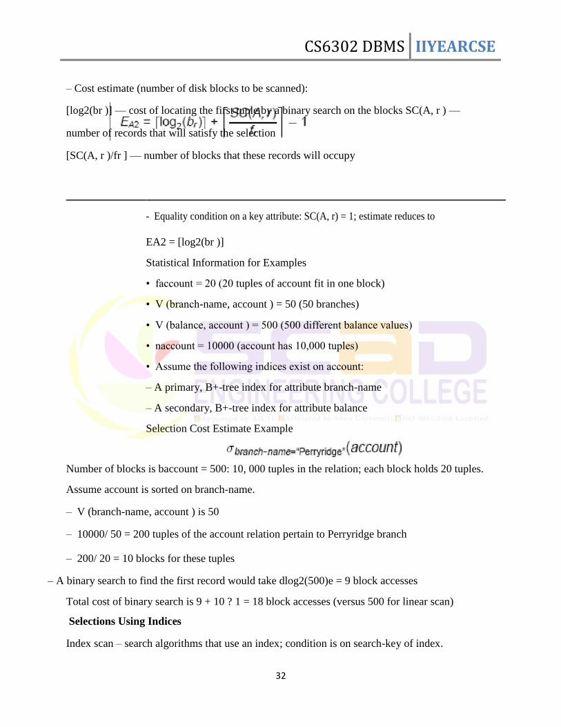
– Cost estimate (number of disk blocks to be scanned): [log2(br )] — cost of locating the first tuple by a binary search on the blocks SC(A, r ) —
number of records that will satisfy the selection
[SC(A, r )/fr ] — number of blocks that these records will occupy
- Equality condition on a key attribute: SC(A, r) = 1; estimate reduces to
EA2 = [log2(br )]
Statistical Information for Examples
• faccount = 20 (20 tuples of account fit in one block)
• V (branch-name, account ) = 50 (50 branches)
• V (balance, account ) = 500 (500 different balance values)
• naccount = 10000 (account has 10,000 tuples)
• Assume the following indices exist on account:
– A primary, B+-tree index for attribute branch-name
– A secondary, B+-tree index for attribute balance
Selection Cost Estimate Example
Number of blocks is baccount = 500: 10, 000 tuples in the relation; each block holds 20 tuples. Assume account is sorted on branch-name. – V (branch-name, account ) is 50 – 10000/ 50 = 200 tuples of the account relation pertain to Perryridge branch – 200/ 20 = 10 blocks for these tuples
– A binary search to find the first record would take dlog2(500)e = 9 block accesses Total cost of binary search is 9 + 10 ? 1 = 18 block accesses (versus 500 for linear scan) Selections Using Indices Index scan – search algorithms that use an index; condition is on search-key of index.
CS6302 DBMS IIYEARCSE
33
A3 (primary index on candidate key, equality). Retrieve a single record that satisfies the
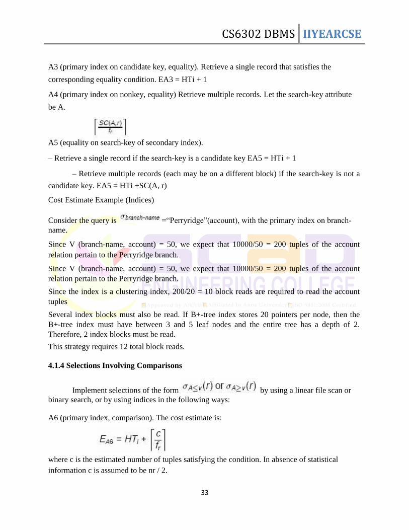
corresponding equality condition. EA3 = HTi + 1 A4 (primary index on nonkey, equality) Retrieve multiple records. Let the search-key attribute
be A.
A5 (equality on search-key of secondary index). – Retrieve a single record if the search-key is a candidate key EA5 = HTi + 1
– Retrieve multiple records (each may be on a different block) if the search-key is not a
candidate key. EA5 = HTi +SC(A, r) Cost Estimate Example (Indices)
Consider the query is =―Perryridge‖(account), with the primary index on branch-
name. Since V (branch-name, account) = 50, we expect that 10000/50 = 200 tuples of the account
relation pertain to the Perryridge branch. Since V (branch-name, account) = 50, we expect that 10000/50 = 200 tuples of the account
relation pertain to the Perryridge branch. Since the index is a clustering index, 200/20 = 10 block reads are required to read the account
tuples Several index blocks must also be read. If B+-tree index stores 20 pointers per node, then the
B+-tree index must have between 3 and 5 leaf nodes and the entire tree has a depth of 2.
Therefore, 2 index blocks must be read. This strategy requires 12 total block reads.
4.1.4 Selections Involving Comparisons
Implement selections of the form by using a linear file scan or
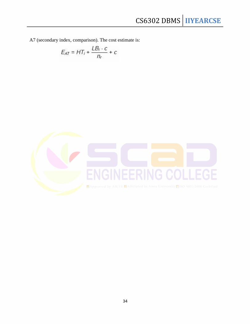
binary search, or by using indices in the following ways: A6 (primary index, comparison). The cost estimate is:
where c is the estimated number of tuples satisfying the condition. In absence of statistical
information c is assumed to be nr / 2.
CS6302 DBMS IIYEARCSE
34
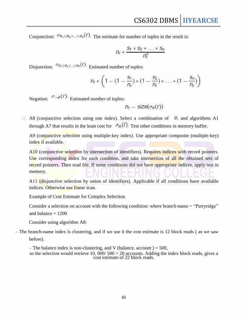
A7 (secondary index, comparison). The cost estimate is:
CS6302 DBMS IIYEARCSE
35
Conjunction: The estimate for number of tuples in the result is:
Disjunction: Estimated number of tuples:
Negation: Estimated number of tuples:
A8 (conjunctive selection using one index). Select a combination of and algorithms A1
through A7 that results in the least cost for Test other conditions in memory buffer.
A9 (conjunctive selection using multiple-key index). Use appropriate composite (multiple-key)
index if available.
A10 (conjunctive selection by intersection of identifiers). Requires indices with record pointers.
Use corresponding index for each condition, and take intersection of all the obtained sets of
record pointers. Then read file. If some conditions did not have appropriate indices, apply test in
memory.
A11 (disjunctive selection by union of identifiers). Applicable if all conditions have available
indices. Otherwise use linear scan. Example of Cost Estimate for Complex Selection Consider a selection on account with the following condition: where branch-name = ―Perryridge‖
and balance = 1200 Consider using algorithm A8:
– The branch-name index is clustering, and if we use it the cost estimate is 12 block reads ( as we saw
before). – The balance index is non-clustering, and V (balance, account ) = 500, so the selection would retrieve 10, 000/ 500 = 20 accounts. Adding the index block reads, gives a
cost estimate of 22 block reads.
CS6302 DBMS IIYEARCSE
36
Optimization: combine tuples in the same group during run generation and intermediate merges, by
computing partial aggregate values. Set operations can either use variant of merge-join after sorting, or variant of hash-join. E.g., Set operations using hashing:
1. Partition both relations using the same hash function, thereby creating Hr0, . . ., Hrmax , and
Hs0, . . ., Hsmax .
2. Process each partition i as follows. Using a different hashing function, build an in-memory hash
index on Hri after it is brought into memory.
3. – r s: Add tuples in Hsi to the hash index if they are not already in it. Then add the tuples in
the hash index to the result.
– r s: output tuples in Hsi to the result if they are already there in the hash index.
– r ? s: for each tuple in Hsi , if it is there in the hash index, delete it from the index. Add
remaining tuples in the hash index to the result. Outer join can be computed either as – A join followed by addition of null-padded non-participating tuples.
Transformation of Relational Expressions
Generation of query-evaluation plans for an expression involves two steps:
1. generating logically equivalent expressions
2. annotating resultant expressions to get alternative query plans Use equivalence rules to transform an expression into an equivalent one. Based on estimated cost, the cheapest plan is selected. The process is called cost based
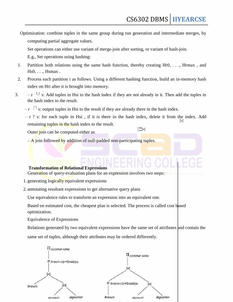
optimization. Equivalence of Expressions Relations generated by two equivalent expressions have the same set of attributes and contain the
same set of tuples, although their attributes may be ordered differently.
CS6302 DBMS IIYEARCSE
37
Equivalent expressions
Equivalence Rules: 1. Conjunctive selection operations can be deconstructed into a sequence of individual selections. __1^_2 (E) = __1 (__2 (E)) 2. Selection operations are commutative. __1 (__2 (E)) = __2 (__1 (E))
3. Only the last in a sequence of projection operations is needed, the others can be omitted. PL1 (PL2 (. . . (PLn (E)) . . .)) = PL1 (E)
For difference and intersection, we also have:
_P (E1 ? E2) = _P (E1) ? E2
12. The projection operation distributes over the union operation.
PL(E1 [ E2) = (PL(E1)) [ (PL(E2))
Selection Operation Example
_ Query: Find the names of all customers who have an account at some branch located
in Brooklyn.
Pcustomer -name (_branch-city = ―Brooklyn‖ (branch 1 (account 1 depositor )))
_ Transformation using rule 7a.
Pcustomer –name ((_branch-city = ―Brooklyn‖ (branch)) 1 (account 1 depositor ))
_ Performing the selection as early as possible reduces the size of the relation to be
joined.
Pcustomer -name((_branch-city = ―Brooklyn‖ (branch) 1 account ) 1 depositor )
_ When we compute (_branch-city = ―Brooklyn‖ (branch) 1 account )
we obtain a relation whose schema is:
(branch-name, branch-city, assets, account-number, balance)
CS6302 DBMS IIYEARCSE
38
_ Push projections using equivalence rules 8a and 8b; eliminate unneeded attributes
from intermediate results to get:
but account 1 depositor is likely to be a large relation.
_ Since it is more likely that only a small fraction of the bank‘s
customers have accounts in branches located in Brooklyn, it is
better to compute
_branch-city = ―Brooklyn‖ (branch) 1 account first.
Evaluation Plan
An evaluation plan defines exactly what algorithm is used for each
operation, and how the execution of the operations is coordinated.
Evaluation Plan Choice of Evaluation Plans Must consider the interaction of evaluation techniques when choosing evaluation plans: choosing
the cheapest algorithm for each operation independently may not yield the best overall algorithm.
E.g. – merge-join may be costlier than hash-join, but may provide a sorted output which reduces the
cost for an outer level aggregation.
nested-loop join may provide opportunity for pipelining
Practical query optimizers incorporate elements of the following two broad approaches:
1. Search all the plans and choose the best plan in a cost-based fashion.
2. Use heuristics to choose a plan. Cost-Based Optimization _ Consider finding the best join-order for r1 1 r2 1 . . . rn. _ There are (2(n ? 1))!/ (n ? 1)! different join orders for above expression. With n = 7, the number
is 665280, with n = 10, the number is greater than 176 billion! _ No need to generate all the join orders. Using dynamic programming, the least-cost join order
for any subset of fr1, r2, . . . , rng is computed only once and stored for future use. _ This reduces time complexity to around O(3n). With n = 10, this number is 59000.
CS6302 DBMS IIYEARCSE
39
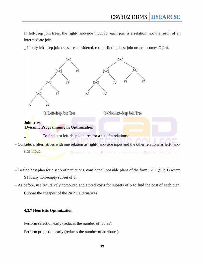
In left-deep join trees, the right-hand-side input for each join is a relation, not the result of an
intermediate join. _ If only left-deep join trees are considered, cost of finding best join order becomes O(2n).
Join trees
Dynamic Programming in Optimization _ To find best left-deep join tree for a set of n relations:
– Consider n alternatives with one relation as right-hand-side input and the other relations as left-hand-
side input.
– To find best plan for a set S of n relations, consider all possible plans of the form: S1 1 (S ?S1) where
S1 is any non-empty subset of S.
– As before, use recursively computed and stored costs for subsets of S to find the cost of each plan.
Choose the cheapest of the 2n ? 1 alternatives.
4.3.7 Heuristic Optimization
Perform selection early (reduces the number of tuples). Perform projection early (reduces the number of attributes)
CS6302 DBMS IIYEARCSE
40
Perform most restrictive selection and join operations before other similar operations.
Steps in Typical Heuristic Optimization
1. Deconstruct conjunctive selections into a sequence of single selection operations (Equiv. rule 1).
2. Move selection operations down the query tree for the earliest possible execution (Equiv. rules 2,
7a, 7b, 11).
3. Execute first those selection and join operations that will produce the smallest relations (Equiv.
rule 6).
4. Replace Cartesian product operations that are followed by a selection condition by join
operations (Equiv. rule 4a).
5. Deconstruct and move as far down the tree as possible lists of projection attributes, creating new
projections where needed (Equiv. rules 3, 8a, 8b, 12).
6. Identify those subtrees whose operations can be pipelined, and execute them using pipelining.
Structure of Query Optimizers _ The System R optimizer considers only left-deep join orders. _ This reduces optimization complexity and generates plans amenable to pipelined evaluation. System R also uses heuristics to push selections and projections down the query tree. _ For scans using secondary indices, the Sybase optimizer takes into account the probability that the page containing the tuple is in the buffer. _ Some query optimizers integrate heuristic selection and the generation of alternative access plans.
– System R and Starburst use a hierarchical procedure based on the nested-block concept of SQL:
heuristic rewriting followed by cost-based join-order optimization. – The Oracle7 optimizer supports a heuristic based on available access paths. _ Even with the use of heuristics, cost-based query optimization imposes a substantial overhead.
This expense is usually more than offset by savings at query-execution time, particularly by reducing the number of slow disk accesses.
CS6302 DBMS IIYEARCSE
41
UNIT III TRANSACTION PROCESSING AND CONCURRENCY CONTROL
TRANSACTION PROCESSING & PROPERTIES Transaction Concept
A transaction is a unit of program execution that accesses and possiblyupdates various data items. A transaction must see a consistent database. During transaction execution the database may be inconsistent. When the transaction is committed, the database must be consistent. Two main issues to deal with:
o Failures of various kinds, such as hardware failures and system crashes o Concurrent execution of multiple transactions
ACID Properties To preserve the integrity of data, the database system must ensure: Atomicity. Either all operations of the transaction are properly reflected in the database or none
are. Consistency. Execution of a transaction in isolation preserves the consistency of the database. Isolation. Although multiple transactions may execute concurrently, each transaction must be
unaware of other concurrently executing transactions. Intermediate transaction results must be
hidden from other concurrently executed transactions. That is, for every pair of transactions Ti
and Tj, it appears to Ti that either Tj finished execution before Ti started, or Tj started execution
after Ti finished.
Durability. After a transaction completes successfully, the changes it has made to the database
persist, even if there are system failures. Example of Fund Transfer Transaction to transfer $50 from account A to account B:
1. read( A)
2. A:= A- 50
3. write( A)
4. read(B)
CS6302 DBMS IIYEARCSE
42
5. B:= B+ 50
6. write( B)
CS6302 DBMS IIYEARCSE
43
Consistency requirement — the sum of A and B is unchanged by the execution of the NOTES transaction. Atomicity requirement — if the transaction fails after step 3 and before step 6, the system
should ensure that its updates are not reflected in the database, else an inconsistency will result. Durability requirement — once the user has been notified that the transaction has completed
(i.e. the transfer of the $50 has taken place), the updates to the database by the transaction must
persist despite failures. Isolation requirement — if between steps 3 and 6, another transaction is allowed to access the
partially updated database, it will see an inconsistent database (the sum A+ B will be less than it
should be). . Example of Supplier Number
• Transaction : logical unit of work
• e.g change supplier number for Sx to Sy;
• The following transaction code must be written: TransX: Proc Options (main); /* declarations omitted */ EXEC SQL WHEREVER SQL-ERROR ROLLBACK; GET LIST (SX, SY); EXEC SQL UPDATE S SET S# =: SY WHERE S# = SX; EXEC SQL UPDATE SP SET S# =: SY WHERE S# = SX; EXEC SQL COMMIT RETURN (); Note: single unit of work here =
2 updates to the DBMS
to 2 separate databases

CS6302 DBMS IIYEARCSE
44
therefore it is
a sequence of several operations which transforms data from one consistent
state to another.
either updates must be performed or none of them E.g. banking.
A.C.I.D
Atomic, Consistent, Isolated, Durable
ACID properties
Atomicity - ‗all or nothing‘, transaction is an indivisible unit that is either performed in its
entirety or not at all
Consistency - a transaction must transform the database from one consistent state to another.
Isolation - transactions execute independently of one another. partial effects of incomplete
transactions should not be visible to other transactions
Durability - effects of a successfully completed (committed) transaction are stored in DB and not
lost because of failure. Transaction Control/concurrency control
vital for maintaining the CONSISTENCY of database
allowing RECOVERY after failure
allowing multiple users to access database CONCURRENTLY
database must not be left inconsistent because of failure mid-tx
other processes should have consistent view of database
completed tx. should be ‗logged‘ by DBMS and rerun if failure. Transaction Boundaries
SQL identifies start of transaction as BEGIN,
end of successful transaction as COMMIT
or ROLLBACK to abort unsuccessful transaction
Oracle allows SAVE POINTS at start of sub-transaction in nested transactions
CS6302 DBMS IIYEARCSE
45
Implementation
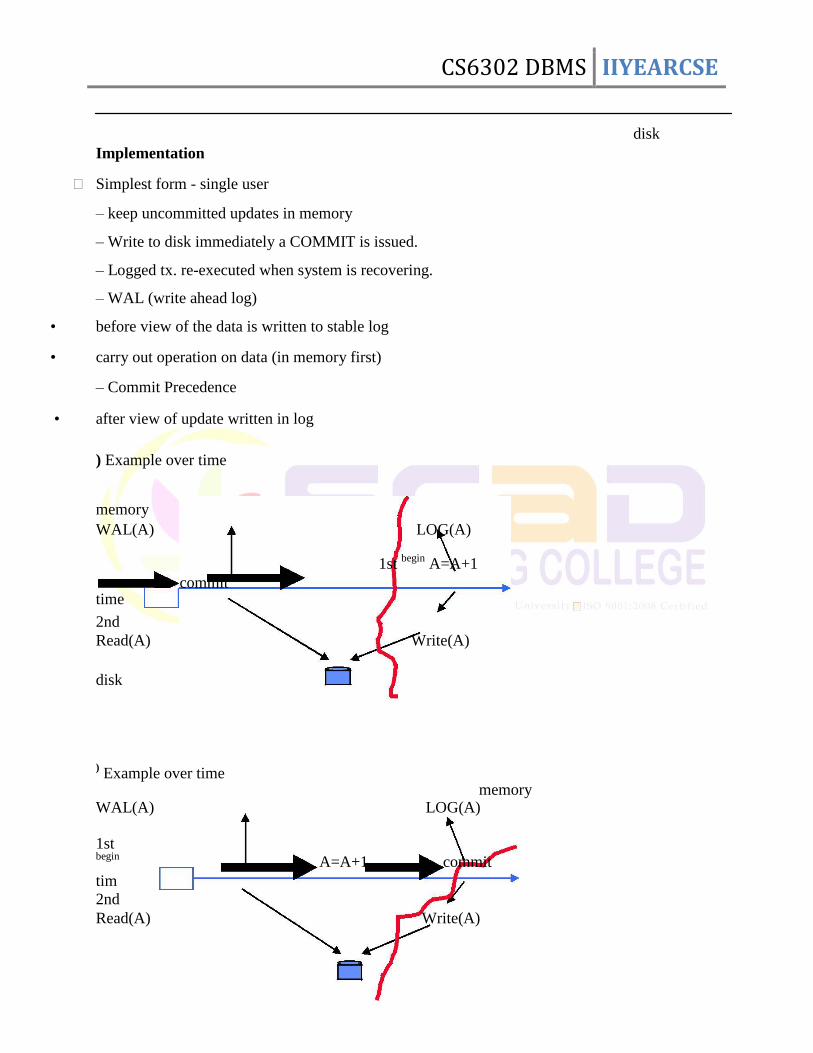
Simplest form - single user – keep uncommitted updates in memory – Write to disk immediately a COMMIT is issued. – Logged tx. re-executed when system is recovering. – WAL (write ahead log)
• before view of the data is written to stable log
• carry out operation on data (in memory first) – Commit Precedence
• after view of update written in log
) Example over time memory WAL(A) LOG(A)
1st begin
A=A+1
commit time 2nd Read(A) Write(A)
disk
) Example over time
memory WAL(A) LOG(A) 1st begin
A=A+1 commit tim
2nd Read(A) Write(A)
disk
CS6302 DBMS IIYEARCSE
46
CS6302 DBMS IIYEARCSE
47
Why the fuss? Multi-user complications consistent view of DB to all other processes
while transaction in progress.
1. Lost Update Problem • Balance of a bank account holds a Bal of £100 • Transaction 1 is withdrawing £10 from a bank account • Transaction 2 is depositing £100 pounds
Time Tx1 Tx2 Bal 1 Begin_transaction 100
2 Begin_transaction Read (bal) 100
3 Read (bal) Bal=bal +100 100
4 Bal = bal – 10 Write (bal) 200
5 Write (bal) Commit 90
6 commit 90
• £100 is lost, so we must prevent T1 from reading the value of Bal until after T2 is finished 2. Uncommitted dependency problem
Time Tx3 Tx4 Bal
1 Begin_transaction 100
2 Read (bal) 100
3 Bal=bal +100 100
4 Begin_transaction Write (bal) 200
5 Read (bal) …. 200 6 Bal = bal –10 Rollback 100 7 Write (bal) 190
8 commit 190 • Transaction 4 needed to abort at time t6
• problem is where transaction is allowed to see intermediate results of another uncommitted
transaction • answer should have been? - £90
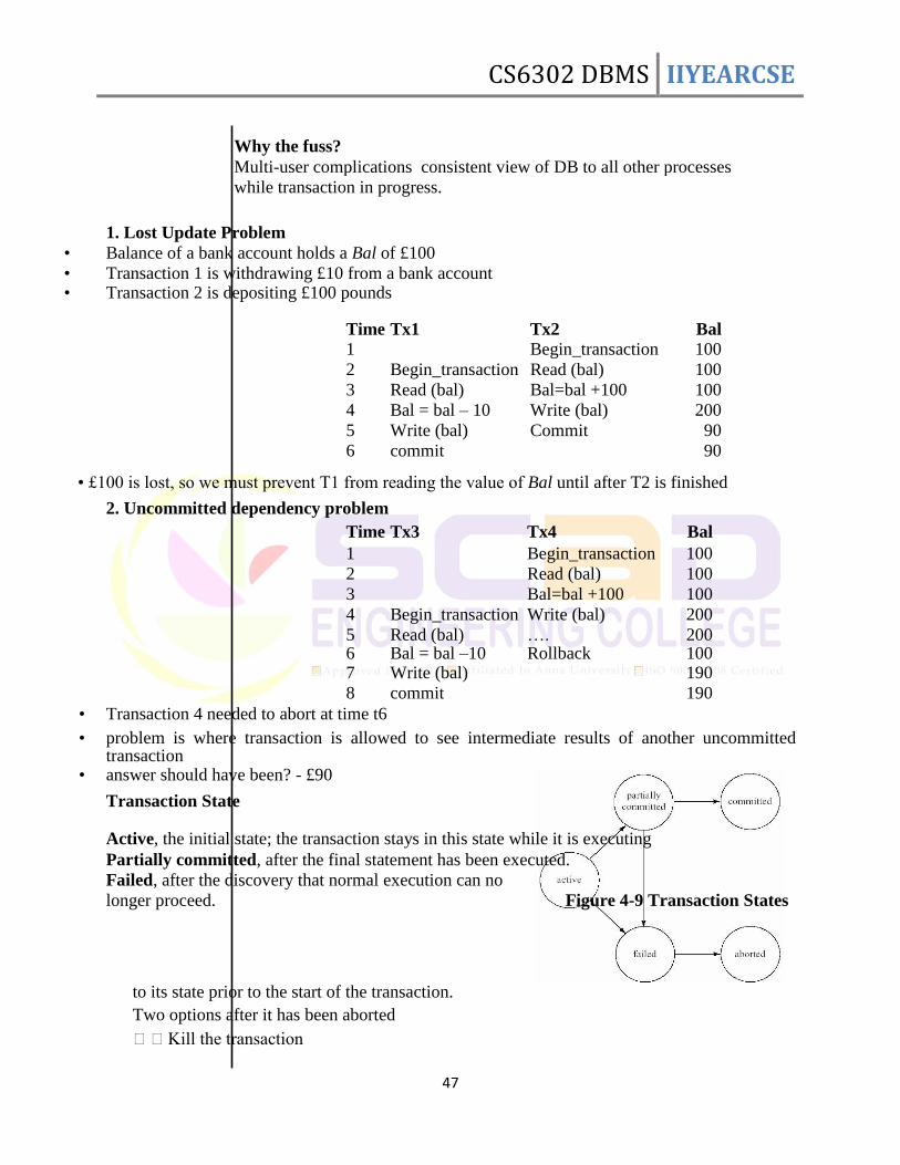
Transaction State
Active, the initial state; the transaction stays in this state while it is executing Partially committed, after the final statement has been executed. Failed, after the discovery that normal execution can no longer proceed. Figure 4-9 Transaction States
to its state prior to the start of the transaction.
Two options after it has been aborted
Kill the transaction
CS6302 DBMS IIYEARCSE
48
Restart the transaction, only if no internal logical error
Committed, after successful completion. Implementation of Atomicity and Durability
The recovery-management component of a database system implements the support for
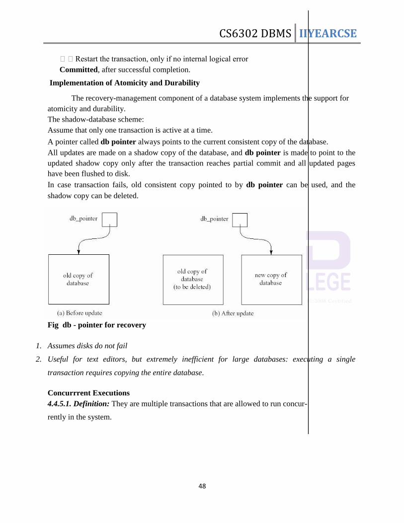
atomicity and durability. The shadow-database scheme: Assume that only one transaction is active at a time. A pointer called db pointer always points to the current consistent copy of the database. All updates are made on a shadow copy of the database, and db pointer is made to point to the
updated shadow copy only after the transaction reaches partial commit and all updated pages
have been flushed to disk. In case transaction fails, old consistent copy pointed to by db pointer can be used, and the
shadow copy can be deleted. Fig db - pointer for recovery
1. Assumes disks do not fail
2. Useful for text editors, but extremely inefficient for large databases: executing a single
transaction requires copying the entire database.
Concurrrent Executions 4.4.5.1. Definition: They are multiple transactions that are allowed to run concur- rently in the system.
CS6302 DBMS IIYEARCSE
49
Advantages of concurrent executions
o Increased processor and disk utilization, leading to better transaction
throughput: one transaction can be using the CPU while another is
reading from or writing to the disk.
o Reduced average response time for transactions: short transactions need
not wait behind long ones.
. Concurrency control schemes:
They are mechanisms to control the interaction among the concurrent transactions
in order to prevent them from destroying the consistency of the database.
. Schedules
Schedules are sequences that indicate the chronological order in which instruc-
tions of concurrent transactions are executed.
A schedule for a set of transactions must consist of all instructions of those
transactions.
Must preserve the order in which the instructions appear in each individual
transaction.
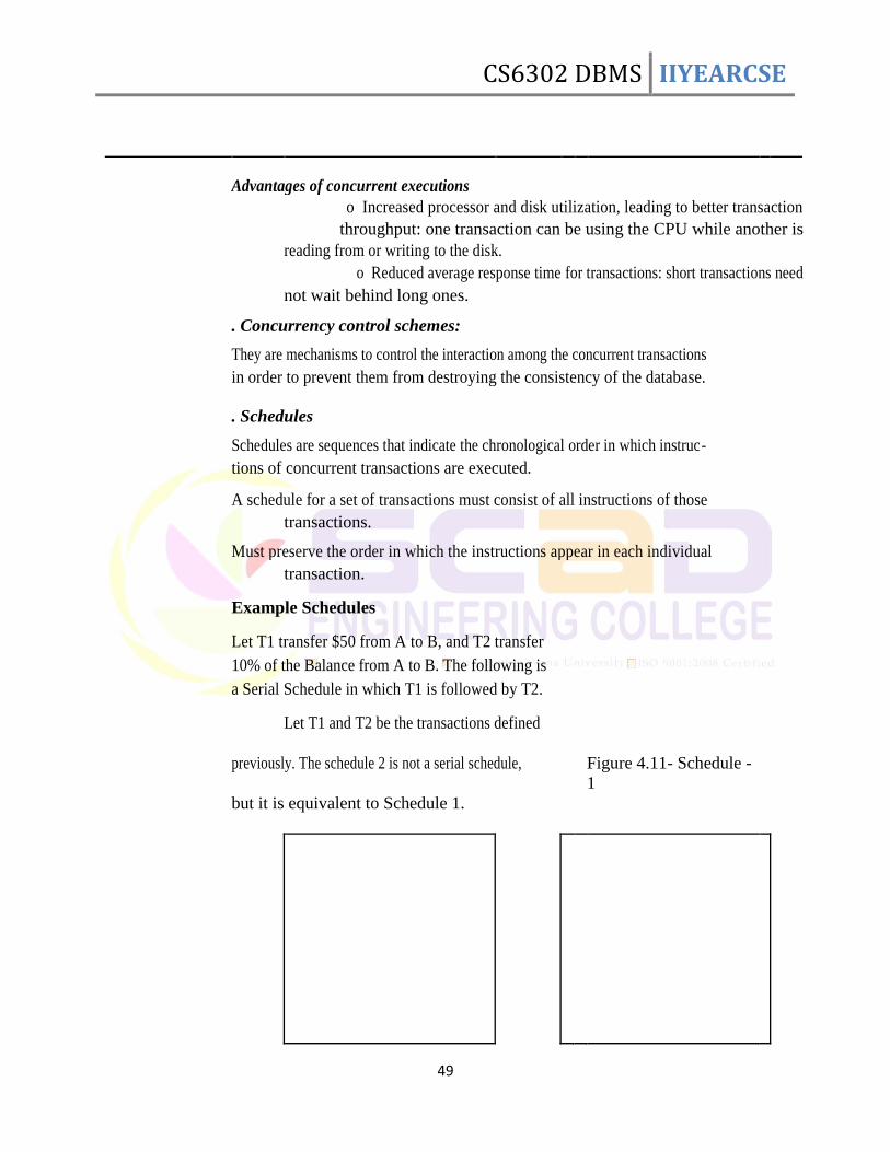
Example Schedules
Let T1 transfer $50 from A to B, and T2 transfer
10% of the Balance from A to B. The following is
a Serial Schedule in which T1 is followed by T2.
Let T1 and T2 be the transactions defined
previously. The schedule 2 is not a serial schedule,
Figure 4.11- Schedule -
1
but it is equivalent to Schedule 1.
CS6302 DBMS IIYEARCSE
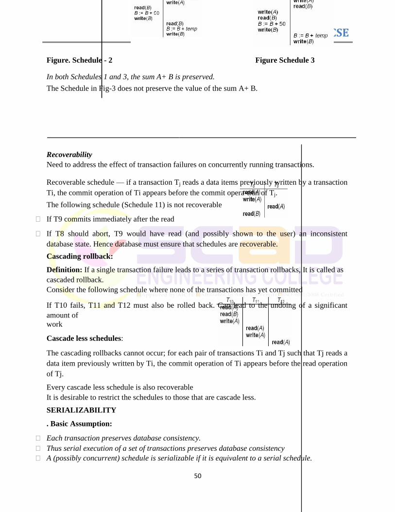
50
Figure. Schedule - 2 Figure Schedule 3 In both Schedules 1 and 3, the sum A+ B is preserved. The Schedule in Fig-3 does not preserve the value of the sum A+ B.
Recoverability Need to address the effect of transaction failures on concurrently running transactions.
Recoverable schedule — if a transaction Tj reads a data items previously written by a transaction
Ti, the commit operation of Ti appears before the commit opera-tion of Tj. The following schedule (Schedule 11) is not recoverable
If T9 commits immediately after the read
If T8 should abort, T9 would have read (and possibly shown to the user) an inconsistent
database state. Hence database must ensure that schedules are recoverable. Cascading rollback: Definition: If a single transaction failure leads to a series of transaction rollbacks, It is called as
cascaded rollback.
Consider the following schedule where none of the transactions has yet committed
If T10 fails, T11 and T12 must also be rolled back. Can lead to the undoing of a significant
amount of work Cascade less schedules: The cascading rollbacks cannot occur; for each pair of transactions Ti and Tj such that Tj reads a
data item previously written by Ti, the commit operation of Ti appears before the read operation
of Tj. Every cascade less schedule is also recoverable It is desirable to restrict the schedules to those that are cascade less. SERIALIZABILITY . Basic Assumption:
Each transaction preserves database consistency. Thus serial execution of a set of transactions preserves database consistency A (possibly concurrent) schedule is serializable if it is equivalent to a serial schedule.
CS6302 DBMS IIYEARCSE
51
Different forms of schedule equivalence give rise to the notions of:
1. Conflict Serializability 2. View Serializability
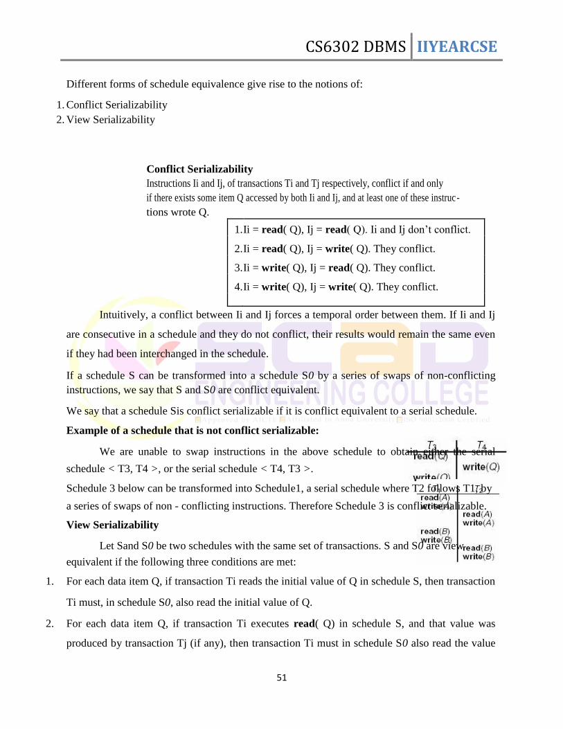
Conflict Serializability
Instructions Ii and Ij, of transactions Ti and Tj respectively, conflict if and only
if there exists some item Q accessed by both Ii and Ij, and at least one of these instruc-
tions wrote Q.
1. Ii = read( Q), Ij = read( Q). Ii and Ij don‘t conflict.
2. Ii = read( Q), Ij = write( Q). They conflict.
3. Ii = write( Q), Ij = read( Q). They conflict.
4. Ii = write( Q), Ij = write( Q). They conflict.
Intuitively, a conflict between Ii and Ij forces a temporal order between them. If Ii and Ij
are consecutive in a schedule and they do not conflict, their results would remain the same even
if they had been interchanged in the schedule. If a schedule S can be transformed into a schedule S0 by a series of swaps of non-conflicting
instructions, we say that S and S0 are conflict equivalent.
We say that a schedule Sis conflict serializable if it is conflict equivalent to a serial schedule. Example of a schedule that is not conflict serializable:
We are unable to swap instructions in the above schedule to obtain either the serial
schedule < T3, T4 >, or the serial schedule < T4, T3 >. Schedule 3 below can be transformed into Schedule1, a serial schedule where T2 follows T1, by
a series of swaps of non - conflicting instructions. Therefore Schedule 3 is conflict serializable. View Serializability
Let Sand S0 be two schedules with the same set of transactions. S and S0 are view
equivalent if the following three conditions are met:
1. For each data item Q, if transaction Ti reads the initial value of Q in schedule S, then transaction
Ti must, in schedule S0, also read the initial value of Q.
2. For each data item Q, if transaction Ti executes read( Q) in schedule S, and that value was
produced by transaction Tj (if any), then transaction Ti must in schedule S0 also read the value
CS6302 DBMS IIYEARCSE
52
of Q that was produced by transaction Tj.
3. For each data item Q, the transaction (if any) that performs the final write (Q) operation in
schedule S must perform the final write (Q) operation in schedule S0.
A schedule S is view serializable if it is view equivalent to a serial schedule. Every conflict
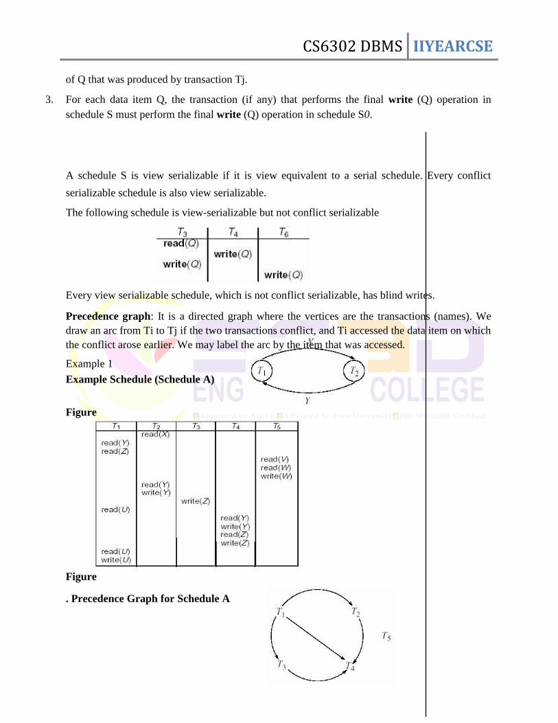
serializable schedule is also view serializable. The following schedule is view-serializable but not conflict serializable
Every view serializable schedule, which is not conflict serializable, has blind writes. Precedence graph: It is a directed graph where the vertices are the transactions (names). We
draw an arc from Ti to Tj if the two transactions conflict, and Ti accessed the data item on which
the conflict arose earlier. We may label the arc by the item that was accessed. Example 1 Example Schedule (Schedule A) Figure
Figure . Precedence Graph for Schedule A
CS6302 DBMS IIYEARCSE
53
CS6302 DBMS IIYEARCSE
54
LOCKING TECHNIQUES Lock-Based Protocols A lock is a mechanism to control concurrent access to a data item. Data items can be locked in two modes: 1. Exclusive (X) mode. Data item can be both read as well as written. X-lock is requested
using lock-X instruction.
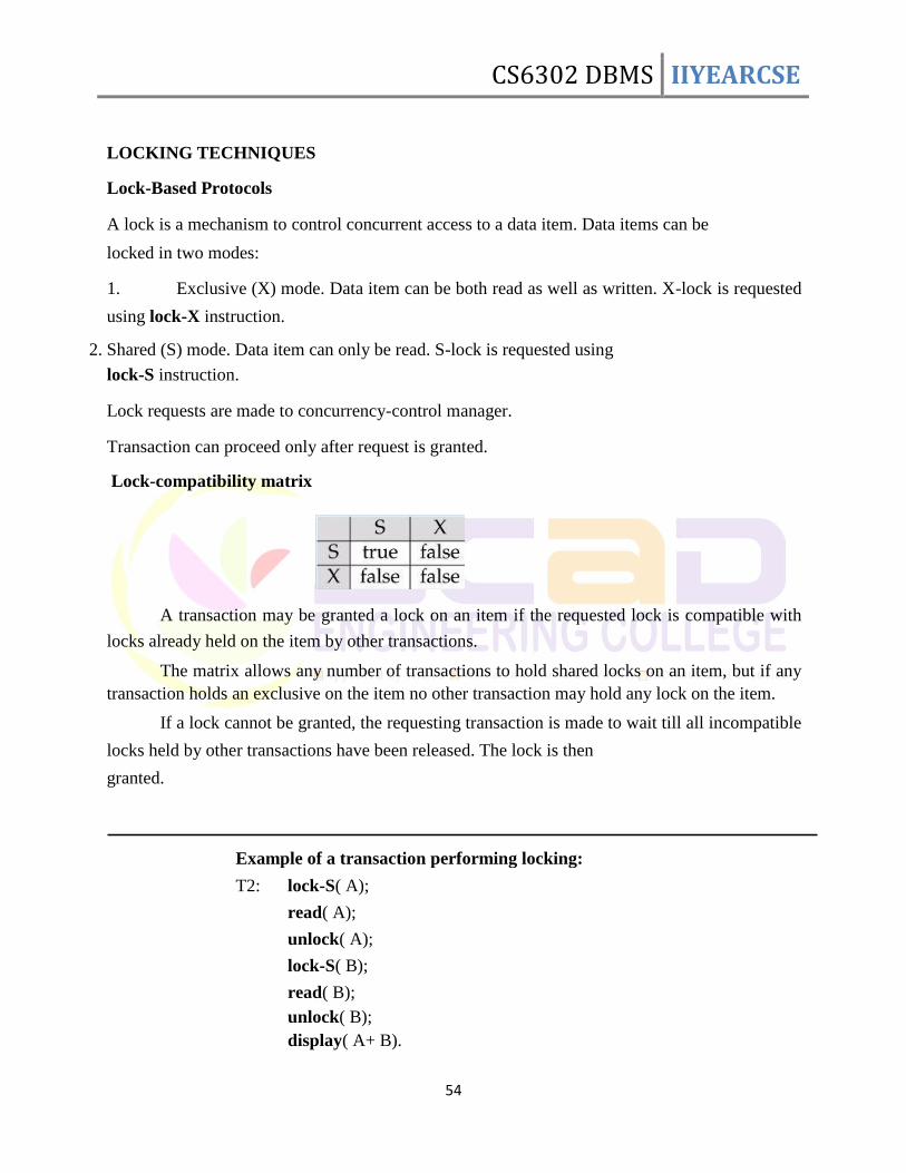
2. Shared (S) mode. Data item can only be read. S-lock is requested using lock-S instruction. Lock requests are made to concurrency-control manager. Transaction can proceed only after request is granted. Lock-compatibility matrix
A transaction may be granted a lock on an item if the requested lock is compatible with
locks already held on the item by other transactions.
The matrix allows any number of transactions to hold shared locks on an item, but if any
transaction holds an exclusive on the item no other transaction may hold any lock on the item.
If a lock cannot be granted, the requesting transaction is made to wait till all incompatible
locks held by other transactions have been released. The lock is then granted.
Example of a transaction performing locking:
T2: lock-S( A);
read( A);
unlock( A);
lock-S( B);
read( B);
unlock( B);
display( A+ B).

CS6302 DBMS IIYEARCSE
55
Locking as above is not sufficient to guarantee serializability.
If A and B get updated in-between the read of A and B, the displayed sum would
be wrong.
A locking protocol is a set of rules followed by all transactions while requesting
and releasing locks. Locking protocols restrict the set of possible schedules.
Pitfalls of Lock-Based Protocols
Consider the partial schedule Neither T3 nor T4 can make progress — executing lock-S( B) causes T4 to wait for T3 to release
its lock on B, while executing lock-X( A) causes T3 to wait for T4 to release its lock on A. Such
a situation is called a deadlock. To handle a deadlock one of T3 or T4 must be rolled back and its locks released. The potential for deadlock exists in most locking protocols. Deadlocks are a necessary evil. . Starvation It is also possible if concurrency control manager is badly designed. For example: A transaction may be waiting for an X-lock on an item, while a sequence of other transactions
request and are granted an S-lock on the same item.
CS6302 DBMS IIYEARCSE
56
The same transaction is repeatedly rolled back due to deadlocks.
Concurrency control manager can be designed to prevent starvation. The Two-Phase Locking Protocol . Introduction This is a protocol, which ensures conflict-serializable schedules. Phase 1: Growing Phase – Transaction may obtain locks. – Transaction may not release locks. Phase 2: Shrinking Phase – Transaction may release locks. – Transaction may not obtain locks.
– The protocol assures serializability. It can be proved that the transactions can be serialized in the
order of their lock points. – Lock points: It is the point where a transaction acquired its final lock. – Two-phase locking does not ensure freedom from deadlocks – Cascading rollback is possible under two-phase locking.
– There can be conflict serializable schedules that cannot be obtained if two-phase locking is used.
Given a transaction Ti that does not follow two-phase locking, we can find a transaction
Tj that uses two-phase locking, and a schedule for Ti and Tj that is not conflict serializable. Lock Conversions Two-phase locking with lock conversions: First Phase: _ can acquire a lock-S on item _ can acquire a lock-X on item _ can convert a lock-S to a lock-X (upgrade)
CS6302 DBMS IIYEARCSE
57
Second Phase:
_ can release a lock-S
_ can release a lock-X
_ can convert a lock-X to a lock-S (downgrade) This protocol assures serializability. But still relies on the programmer to insert the various
locking instructions. Automatic Acquisition of Locks A transaction Ti issues the standard read/write instruction, without explicit locking calls.
The operation read( D) is processed as: if Ti has a lock on D then read( D) else begin if necessary wait until no other transaction has a lock-X on D grant Ti a lock-S on D; read( D) end; write( D) is processed as: if Ti has a lock-X on D
then write( D) else begin if necessary wait until no other trans. has any lock on D, if Ti has a lock-S on D then upgrade lock on Dto lock-X else grant Ti a lock-X on D write( D) end;All locks are released after commit or abort
CS6302 DBMS IIYEARCSE
58
. Graph-Based Protocols It is an alternative to two-phase locking.
Impose a partial ordering on the set D = f d1, d2 , ..., dhg of all data items. If di! dj, then any transaction accessing both di and dj must access di before accessing dj.
Implies that the set D may now be viewed as a directed acyclic graph, called a database graph.
Tree-protocol is a simple kind of graph protocol.
Tree Protocol Only exclusive locks are allowed.
The first lock by Ti may be on any data item. Subsequently, Ti can lock a data item Q, only if Ti
currently locks the parent of Q.
Data items may be unlocked at any time.
A data item that has been locked and unlocked by Ti cannot subsequently be re-locked by Ti.
The tree protocol ensures conflict serializability as well as freedom from deadlock.
Unlocking may occur earlier in the tree-locking protocol than in the two-phase locking protocol.
Shorter waiting times, and increase in concurrency.
Protocol is deadlock-free.
However, in the tree-locking protocol, a transaction may have to lock data items that it does not
access.
Increased locking overhead, and additional waiting time.
Potential decrease in concurrency.
Schedules not possible under two-phase locking are possible under tree protocol, and vice versa. Locks
Exclusive – intended to write or modify database – other processes may read but not update it – Oracle sets Xlock before INSERT/DELETE/UPDATE – explicitly set for complex transactions to avoid Deadlock
CS6302 DBMS IIYEARCSE
59
Shared
– read lock, set by many transactions simultaneously
– Xlock can‘t be issued while Slock on
– Oracle automatically sets Slock
– explicitly set for complex transactions to avoid Deadlock
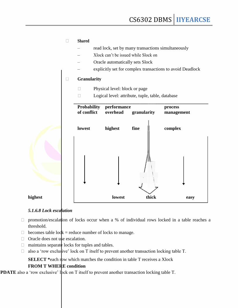
Granularity
Physical level: block or page
Logical level: attribute, tuple, table, database
Probability performance process
of conflict overhead granularity management
lowest
highest fine
complex
highest lowest thick easy 5.1.6.8 Lock escalation
promotion/escalation of locks occur when a % of individual rows locked in a table reaches a
threshold. becomes table lock = reduce number of locks to manage. Oracle does not use escalation. maintains separate locks for tuples and tables. also a ‗row exclusive‘ lock on T itself to prevent another transaction locking table T.
SELECT *each row which matches the condition in table T receives a Xlock FROM T WHERE condition
FOR UPDATE also a ‗row exclusive‘ lock on T itself to prevent another transaction locking table T.
CS6302 DBMS IIYEARCSE
60
this statement explicitly identifies a set of rows which will be used to update another table in the
database, and whose values must remain unchanged throughout the rest of the transaction.
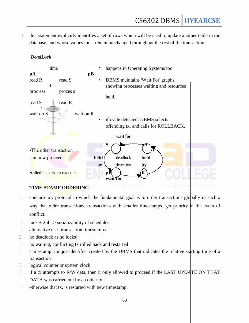
DeadLock
•
pA
time
pB
happens in Operating Systems too
• DBMS maintains 'Wait For' graphs
read R
R
read S
proc ess proces s
showing processes waiting and resources
held.
read S
S
read R
•
wait on S wait on R
if cycle detected, DBMS selects
offending tx. and calls for ROLLBACK.
wait for
•The other transaction
S pA
can now proceed. held deadlock held
•rolled back tx. re-executes.
by detection by
pB R
wait for TIME STAMP ORDERING
concurrency protocol in which the fundamental goal is to order transactions globally in such a
way that older transactions, transactions with smaller timestamps, get priority in the event of
conflict.
lock + 2pl => serializability of schedules
alternative uses transaction timestamps
no deadlock as no locks!
no waiting, conflicting tx rolled back and restarted
Timestamp: unique identifier created by the DBMS that indicates the relative starting time of a
transaction
logical counter or system clock
if a tx attempts to R/W data, then it only allowed to proceed if the LAST UPDATE ON THAT
DATA was carried out by an older tx.
otherwise that tx. is restarted with new timestamp.
CS6302 DBMS IIYEARCSE
61
Data also has timestamps, read and write
Test for Conflict Serializability
A schedule is conflict serializable if and only if its precedence graph is acyclic.
Cycle-detection algorithms exist which take order n2 time, where n is the number of
vertices in the graph.
If precedence graph is acyclic, the serializability order can be obtained by a
topological sorting of the graph. This is a linear order consistent with the partial order of
the graph.
For example, a Serializability order for Schedule A would be T5 T1 T3 T2 T4.
Test for View Serializability
The precedence graph test for conflict serializability must be modified to apply
to a test for view serializability.
Construct a labeled precedence graph. Look for an acyclic graph, which is
derived from the labeled precedence graph by choosing one edge from every pair of
edges with the same non-zero label. Schedule is view serializable if and only if such an
acyclic graph can be found.
The problem of looking for such an acyclic graph falls in the class of NP-
complete problems. Thus existence of an efficient algorithm is unlikely.
However practical algorithms that just check some sufficient conditions for UNIT IV
TRENDS IN DATABASE TECHNOLOGY
Classification of Physical Storage Media Based on Speed with which data can be accessed
Based on Cost per unit of data Based on Reliability Data loss on power failure or system crash
Physical failure of the storage device H Based on life of
storage
Volatile storage: loses contents when power is switched
off 4 Non-volatile storage: Contents persist even when power is
switched off. Includes secondary and tertiary
storage, as well as batter- backed up main-memory.

CS6302 DBMS IIYEARCSE
62
Physical Storage Media Cache
4 The fastest and most costly form of storage
4 Volatile
4 Managed by the computer system hardware. Main memory 4 Fast access (10s to 100s of nanoseconds; 1 nanosecond
= 10–9 seconds) 4 Generally too small (or too expensive)
to store the entire database
Capacities of up to a few Gigabytes
widely used currently Capacities have gone up and per-byte costs have
decreased steadily and rapidly
Volatile — contents of main memory are usually lost if a
power failure or system crash occurs.
Flash memory
4 Data survives power failure
4 Data can be written at a location only once, but location can be erased
and written to again
4 Can support only a limited number of write/erase cycles.
4 Erasing of memory has to be done to an entire bank of memory.
4 Reads are roughly as fast as main memory
4 But writes are slow (few microseconds), erase is slower
4 Cost per unit of storage roughly similar to main memory
4 Widely used in embedded devices such as digital cameras
4 Also known as EEPROM Magnetic-disk Data is stored on spinning disk,
and read/written magnetically Primary medium for the long-term storage of data;
typically stores entire database. Data must be moved from disk to main memory for
CS6302 DBMS IIYEARCSE
63
access, and written back for storage Much slower access
than main memory (more on this later)
Direct-access – possible to read data on disk in any order,
unlike magnetic tape Hard disks vs. floppy disks Capacities range up to roughly
100 GB currently Much larger capacity and cost/byte than main
memory/ flash memory Growing constantly
and rapidly with technology improvements Survives power failures and
system crashes Disk failure can
destroy data, but is very rare. Optical storage Non-volatile, data is read
optically from a spinning disk using a laser CD-ROM (640 MB) and DVD
(4.7 to 17 GB) most popular forms Write-one, read-many (WORM) optical disks used for
archival storage (CD-R and DVD-R) 4 Multiple write versions also available (CD-RW, DVD-
RW, and DVD-RAM) 4 Reads and writes are slower than
with magnetic disk Juke-box systems, with large numbers of removable
disks, a few drives, and a mechanism for automatic
loading/unloading of disks available for storing large
volumes of data.
Optical Disks Compact disk-read only memory (CD-ROM) 4 Disks can be loaded into or removed from a drive 4
High storage capacity (640 MB per disk)
CS6302 DBMS IIYEARCSE
64
4 High seek times or about 100 msec (optical read
head is heavier and slower) Higher latency (3000 RPM) and lower data-transfer rates
(3-6 MB/s) compared to magnetic disks Digital Video Disk (DVD) DVD-5 holds 4.7 GB, and DVD-9 holds 8.5 GB DVD-10 and DVD-18 are double sided formats with
capacities of 9.4 GB & 17 GB
Other characteristics similar to CD-ROM 4 Record once
versions (CD-R and DVD-R)
Data can only be written once, and cannot be
erased. High capacity and long lifetime; used for archival
storage 4Multi-write versions (CD-RW, DVD-RW and DVD-
RAM) also available Tape storage
Non-volatile, used primarily for backup (to recover from
disk failure), and for archival data
Sequential-access – much slower than disk Very high capacity (40 to 300 GB tapes available) Tape can be removed from drive storage costs much
cheaper than disk, but drives are expensive 4 Tape jukeboxes available for storing massive
amounts of data Hundreds of terabytes (1 terabyte = 109 bytes) to even a
petabyte (1 petabyte = 1012 bytes)
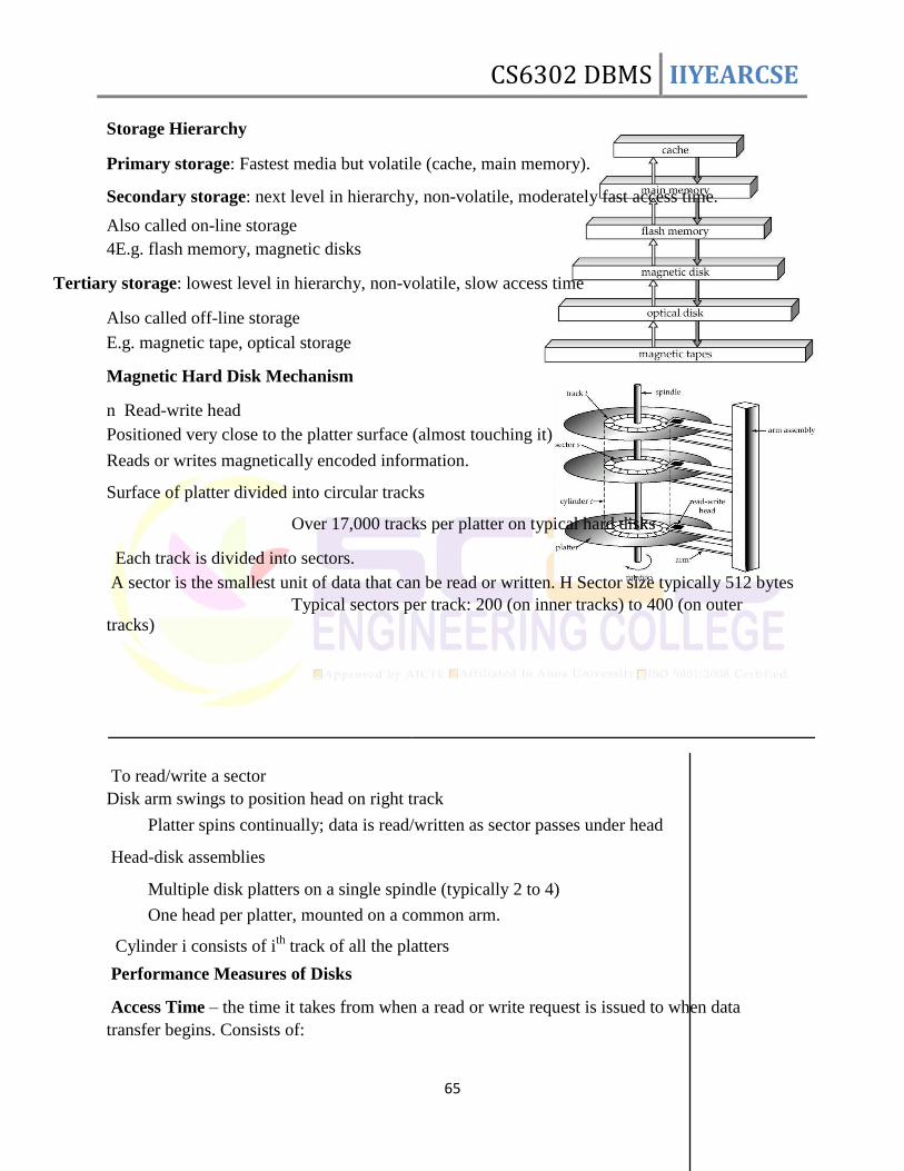
CS6302 DBMS IIYEARCSE
65
Storage Hierarchy Primary storage: Fastest media but volatile (cache, main memory). Secondary storage: next level in hierarchy, non-volatile, moderately fast access time. Also called on-line storage 4E.g. flash memory, magnetic disks
Tertiary storage: lowest level in hierarchy, non-volatile, slow access time Also called off-line storage E.g. magnetic tape, optical storage Magnetic Hard Disk Mechanism n Read-write head
Positioned very close to the platter surface (almost touching it) Reads or writes magnetically encoded information. Surface of platter divided into circular tracks Over 17,000 tracks per platter on typical hard disks Each track is divided into sectors. A sector is the smallest unit of data that can be read or written. H Sector size typically 512 bytes
Typical sectors per track: 200 (on inner tracks) to 400 (on outer
tracks)
To read/write a sector Disk arm swings to position head on right track Platter spins continually; data is read/written as sector passes under head Head-disk assemblies Multiple disk platters on a single spindle (typically 2 to 4) One head per platter, mounted on a common arm. Cylinder i consists of i
th track of all the platters
Performance Measures of Disks Access Time – the time it takes from when a read or write request is issued to when data
transfer begins. Consists of:
CS6302 DBMS IIYEARCSE
66
Seek Time – time it takes to reposition the arm over the correct track. Average Seek Time is 1/2 the worst case seek time.
– Would be 1/3 if all tracks had the same number of sectors, and we ignore the time to start and stop arm movement 4 to 10 milliseconds on typical disks Rotational latency – time it takes for the sector to be accessed to appear under the head. Average latency is 1/2 of the worst-case latency. 4 to 11 milliseconds on typical disks (5400 to 15000 r.p.m.) n Data-Transfer Rate – the rate at which data can be retrieved from or stored to the disk. H4 to 8 MB per second is typical Multiple disks may share a controller, so rate that controller can handle is also important Mean Time To Failure (MTTF) – the average time the disk is expected to run continuously
without any failure. Typically 3 to 5 years Probability of failure of new disks is quite low, corresponding to a ―theoretical MTTF‖ of
30,000 to 1,200,000 hours for a new disk. RAID RAID: Redundant Arrays of Independent Disks disk organization techniques that manage a large numbers of disks, providing a view of a single
disk of
high reliability by storing data redundantly, so that data can be recovered even if a disk fails.
The chance that some disk out of a set of N disks will fail is much higher than the chance that a
specific single disk will fail.
E.g., a system with 100 disks, each with MTTF of 100,000 hours (approx. 11 years), will have a
system MTTF of 1000 hours (approx. 41 days)
o Techniques for using redundancy to avoid data loss are critical with large numbers of disks
Originally a cost-effective alternative to large, expensive disks.
o I in RAID originally stood for ―inexpensive‘‘
o Today RAIDs are used for their higher reliability and bandwidth.
The ―I‖ is interpreted as independent
Improvement of Reliability via Redundancy
Redundancy – store extra information that can be used to rebuild information lost in a disk
CS6302 DBMS IIYEARCSE
67
failure.
E.g., Mirroring (or shadowing) o Duplicate every disk. Logical disk consists of two physical disks. o Every write is carried out on both disks
Reads can take place from either disk o If one disk in a pair fails, data still available in the other
Data loss would occur only if a disk fails, and its mirror disk also fails before the system is
repaired.
Probability of combined event is very small o Except for dependent failure modes such as fire or building collapse or electrical power surges.
Mean time to data loss depends on mean time to failure, and mean time to repair.
o E.g. MTTF of 100,000 hours, mean time to repair of 10 hours
gives mean time to data loss of 500*106 hours (or 57,000 years)
for a mirrored pair of disks (ignoring dependent failure modes)
Improvement in Performance via Parallelism o Two main goals of parallelism in a disk system:
1. Load balance multiple small accesses to increase throughput 2. Parallelize large accesses to reduce response time.
o Improve transfer rate by striping data across multiple disks.
o Bit-level striping – split the bits of each byte across multiple disks
In an array of eight disks, write bit i of each byte to disk i. Each access can read data at eight times the rate of a single disk.
But seek/access time worse than for a single disk
Bit level striping is not used much any more
o Block-level striping – with n disks, block i of a file goes to disk (i mod n) + 1
Requests for different blocks can run in parallel if the blocks reside on different disks.
A request for a long sequence of blocks can utilize all disks in parallel. RAID Levels
o Schemes to provide redundancy at lower cost by using disk striping combined with parity bits.
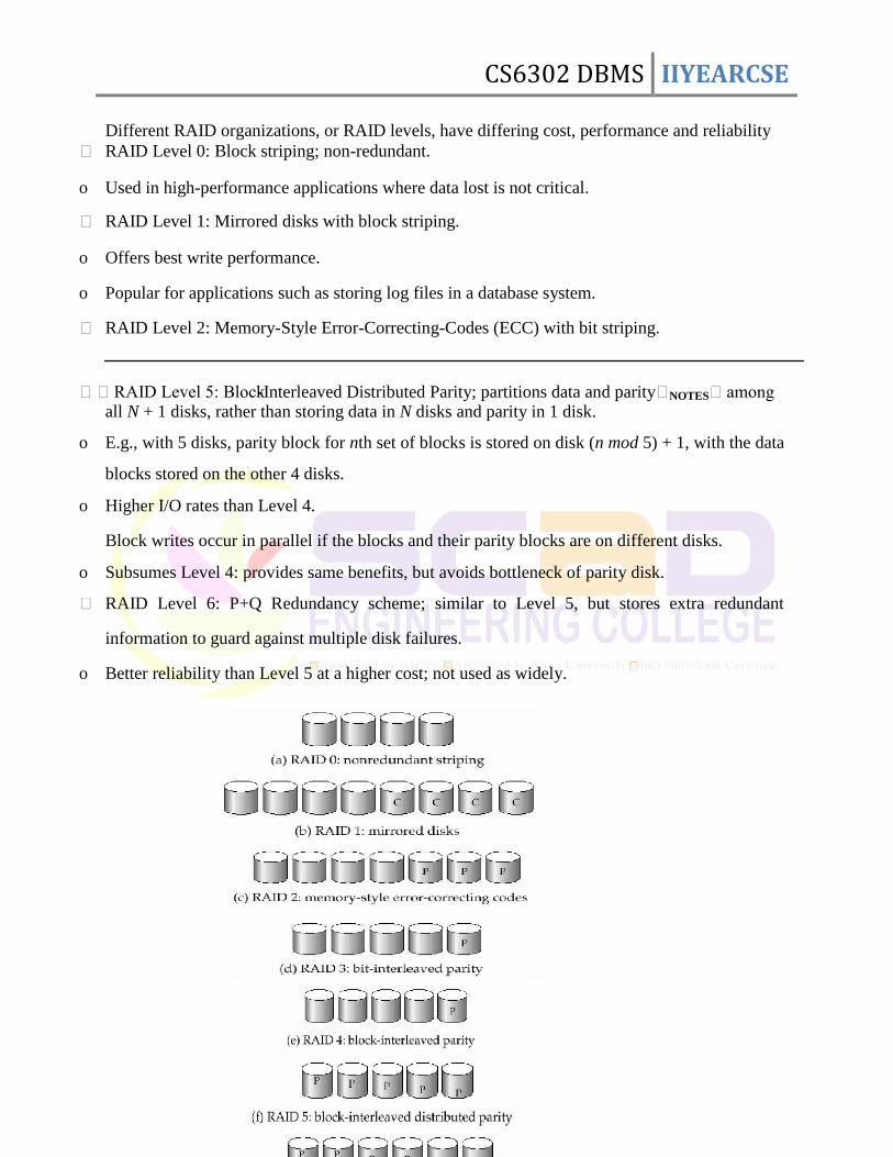
CS6302 DBMS IIYEARCSE
68
Different RAID organizations, or RAID levels, have differing cost, performance and reliability
RAID Level 0: Block striping; non-redundant.
o Used in high-performance applications where data lost is not critical.
RAID Level 1: Mirrored disks with block striping.
o Offers best write performance.
o Popular for applications such as storing log files in a database system.
RAID Level 2: Memory-Style Error-Correcting-Codes (ECC) with bit striping.
RAID Level 5: Block-Interleaved Distributed Parity; partitions data and parityNOTESamong all N + 1 disks, rather than storing data in N disks and parity in 1 disk.
o E.g., with 5 disks, parity block for nth set of blocks is stored on disk (n mod 5) + 1, with the data
blocks stored on the other 4 disks.
o Higher I/O rates than Level 4.
Block writes occur in parallel if the blocks and their parity blocks are on different disks.
o Subsumes Level 4: provides same benefits, but avoids bottleneck of parity disk.
RAID Level 6: P+Q Redundancy scheme; similar to Level 5, but stores extra redundant
information to guard against multiple disk failures.
o Better reliability than Level 5 at a higher cost; not used as widely.

CS6302 DBMS IIYEARCSE
69
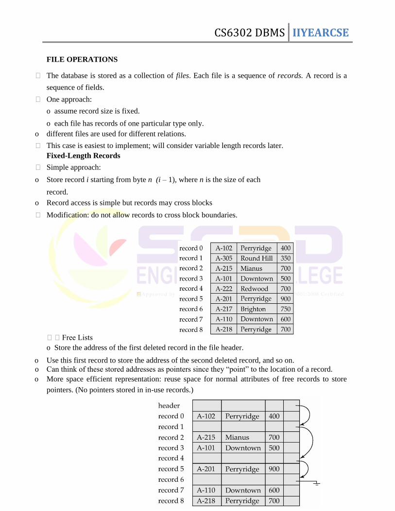
CS6302 DBMS IIYEARCSE
70
FILE OPERATIONS
The database is stored as a collection of files. Each file is a sequence of records. A record is a
sequence of fields.
One approach: o assume record size is fixed. o each file has records of one particular type only.
o different files are used for different relations.
This case is easiest to implement; will consider variable length records later. Fixed-Length Records
Simple approach:
o Store record i starting from byte n (i – 1), where n is the size of each record.
o Record access is simple but records may cross blocks
Modification: do not allow records to cross block boundaries.
Free Lists o Store the address of the first deleted record in the file header.
o Use this first record to store the address of the second deleted record, and so on. o Can think of these stored addresses as pointers since they ―point‖ to the location of a record. o More space efficient representation: reuse space for normal attributes of free records to store
pointers. (No pointers stored in in-use records.)
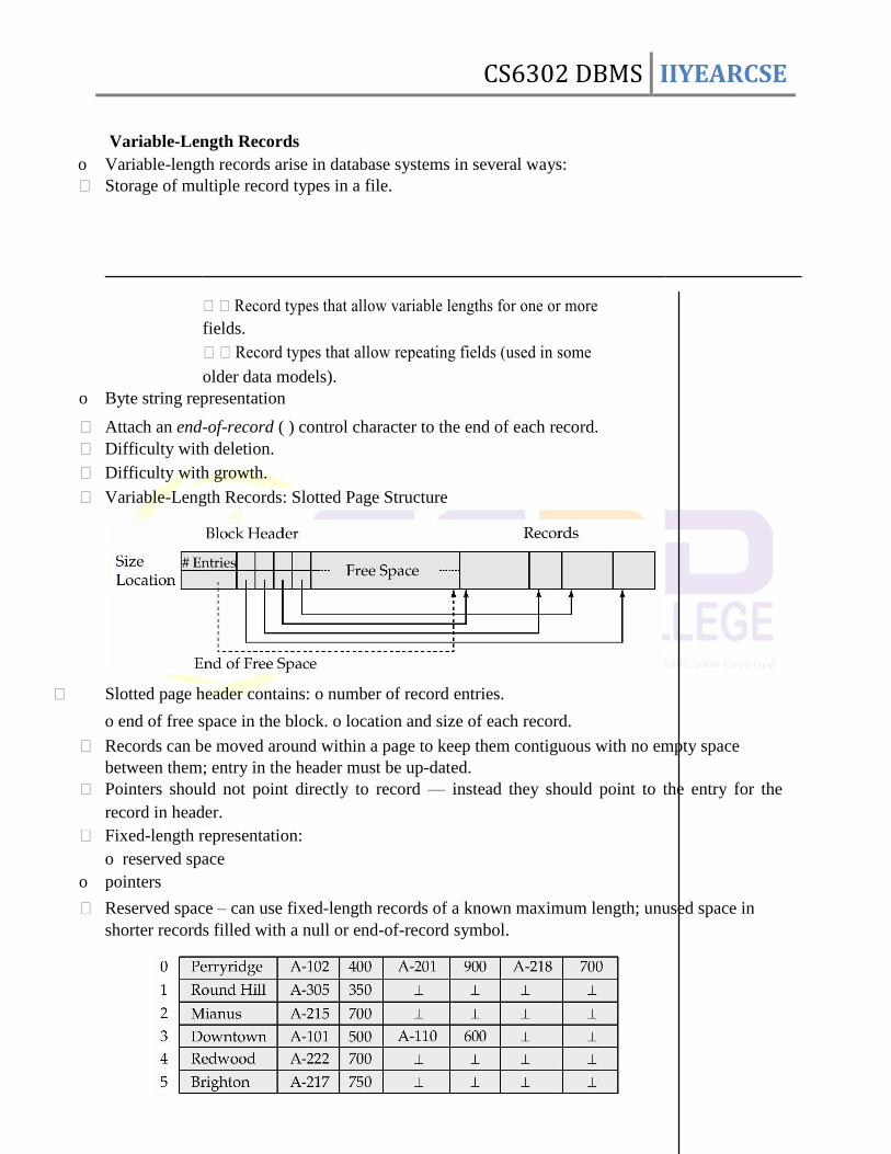
CS6302 DBMS IIYEARCSE
71
Variable-Length Records
o Variable-length records arise in database systems in several ways: Storage of multiple record types in a file.
Record types that allow variable lengths for one or more
fields.
Record types that allow repeating fields (used in some
older data models). o Byte string representation
Attach an end-of-record ( ) control character to the end of each record. Difficulty with deletion. Difficulty with growth. Variable-Length Records: Slotted Page Structure
Slotted page header contains: o number of record entries. o end of free space in the block. o location and size of each record.
Records can be moved around within a page to keep them contiguous with no empty space
between them; entry in the header must be up-dated. Pointers should not point directly to record — instead they should point to the entry for the
record in header. Fixed-length representation:
o reserved space o pointers
Reserved space – can use fixed-length records of a known maximum length; unused space in
shorter records filled with a null or end-of-record symbol.

CS6302 DBMS IIYEARCSE
72
Pointer Method
Pointer method
A variable-length record is represented by a list of fixed-length records, chained together via
pointers.
Can be used even if the maximum record length is not known Disadvantage to pointer structure; space is wasted in all records except the first in a a chain.
Solution is to allow two kinds of block in file: Anchor block – contains the first records of chain Overflow block – contains records other than those that are the first records of chairs.
Organization of Records in Files Heap – a record can be placed anywhere in the file where there is space Sequential – store records in sequential order, based on the value of the search key of each record Hashing – a hash function computed on some attribute of each record; the result specifies in
which block of the file the record should be placed
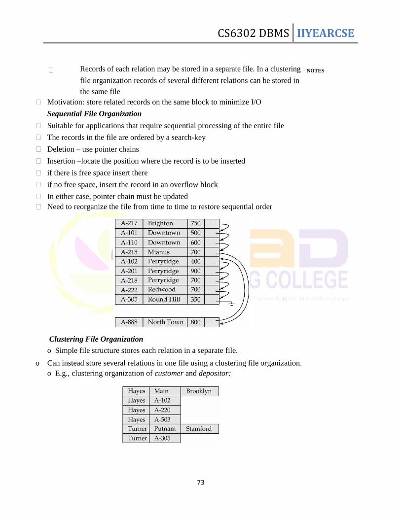
CS6302 DBMS IIYEARCSE
73
Records of each relation may be stored in a separate file. In a clustering NOTES
file organization records of several different relations can be stored in
the same file Motivation: store related records on the same block to minimize I/O
Sequential File Organization
Suitable for applications that require sequential processing of the entire file
The records in the file are ordered by a search-key
Deletion – use pointer chains
Insertion –locate the position where the record is to be inserted
if there is free space insert there
if no free space, insert the record in an overflow block
In either case, pointer chain must be updated Need to reorganize the file from time to time to restore sequential order
Clustering File Organization o Simple file structure stores each relation in a separate file.
o Can instead store several relations in one file using a clustering file organization. o E.g., clustering organization of customer and depositor:
CS6302 DBMS IIYEARCSE
74
Mapping of Objects to Files
Mapping objects to files is similar to mapping tuples to files in a relational system; object data
can be stored using file structures.
Objects in O-O databases may lack uniformity and may be very large; such objects have to
managed differently from records in a relational system.
o Set fields with a small number of elements may be implemented using data structures such as
linked lists.
o Set fields with a larger number of elements may be implemented as separate relations in the
database. o Set fields can also be eliminated at the storage level by normalization. Similar to conversion of multivalued attributes of E-R diagrams to relations
Objects are identified by an object identifier (OID); the storage system needs a mechanism to
locate an object given its OID (this action is called dereferencing).
o logical identifiers do not directly specify an object‘s physical location; must maintain an index that
maps an OID to the object‘s actual location. o physical identifiers encode the location of the object so the object can be found directly. Physical
OIDs typically have the following parts: 1. a volume or file identifier 2. a page identifier within the volume or file 3. an offset within the page
HASHING Hashing is a hash function computed on some attribute of each record; the result specifies in
which block of the file the record should be placed.
Static Hashing A bucket is a unit of storage containing one or more records (a bucket is typically a disk block).
Hash function h is a function from the set of all search-key values K to the set of all bucket
addresses B. Hash function is used to locate records for access, insertion as well as deletion.
Records with different search-key values may be mapped to the same bucket; thus entire bucket
has to be searched sequentially to locate a record. Example of Hash File Organization
Hash file organization ofaccountfile, usingbranch-nameas keyo There are 10 buckets,
o The binary representation of the ith character is assumed to be the integer i. o The hash function returns the sum of the binary representations of the characters modulo 10.
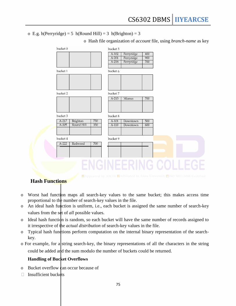
CS6302 DBMS IIYEARCSE
75
o E.g. h(Perryridge) = 5 h(Round Hill) = 3 h(Brighton) = 3
o Hash file organization of account file, using branch-name as key
Hash Functions
o Worst had function maps all search-key values to the same bucket; this makes access time
proportional to the number of search-key values in the file. o An ideal hash function is uniform, i.e., each bucket is assigned the same number of search-key
values from the set of all possible values.
o Ideal hash function is random, so each bucket will have the same number of records assigned to
it irrespective of the actual distribution of search-key values in the file. o Typical hash functions perform computation on the internal binary representation of the search-
key.
o For example, for a string search-key, the binary representations of all the characters in the string
could be added and the sum modulo the number of buckets could be returned. Handling of Bucket Overflows
o Bucket overflow can occur because of
Insufficient buckets
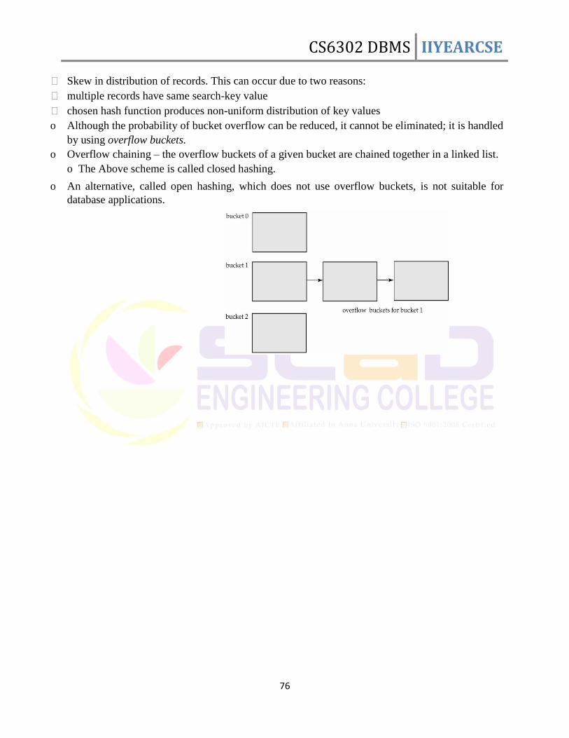
CS6302 DBMS IIYEARCSE
76
Skew in distribution of records. This can occur due to two reasons: multiple records have same search-key value chosen hash function produces non-uniform distribution of key values o Although the probability of bucket overflow can be reduced, it cannot be eliminated; it is handled
by using overflow buckets. o Overflow chaining – the overflow buckets of a given bucket are chained together in a linked list.
o The Above scheme is called closed hashing.
o An alternative, called open hashing, which does not use overflow buckets, is not suitable for
database applications.
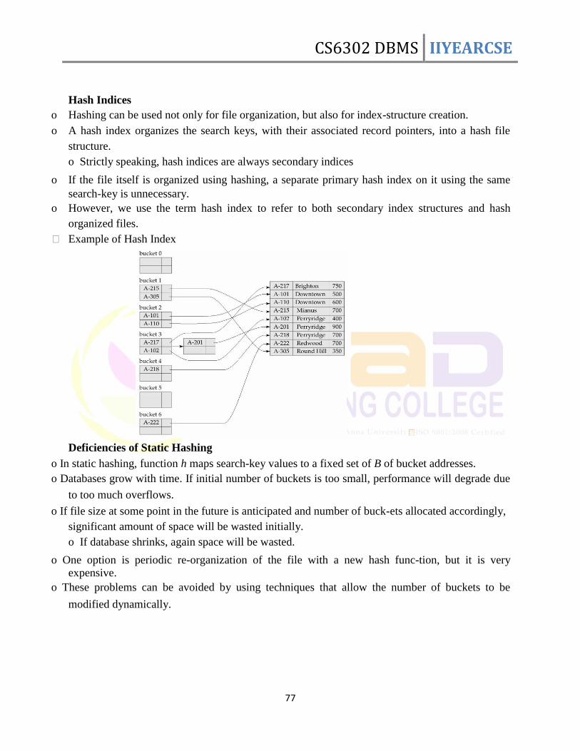
CS6302 DBMS IIYEARCSE
77
Hash Indices o Hashing can be used not only for file organization, but also for index-structure creation.
o A hash index organizes the search keys, with their associated record pointers, into a hash file
structure. o Strictly speaking, hash indices are always secondary indices
o If the file itself is organized using hashing, a separate primary hash index on it using the same
search-key is unnecessary. o However, we use the term hash index to refer to both secondary index structures and hash
organized files.
Example of Hash Index
Deficiencies of Static Hashing o In static hashing, function h maps search-key values to a fixed set of B of bucket addresses. o Databases grow with time. If initial number of buckets is too small, performance will degrade due
to too much overflows.
o If file size at some point in the future is anticipated and number of buck-ets allocated accordingly,
significant amount of space will be wasted initially. o If database shrinks, again space will be wasted.
o One option is periodic re-organization of the file with a new hash func-tion, but it is very expensive.
o These problems can be avoided by using techniques that allow the number of buckets to be
modified dynamically.
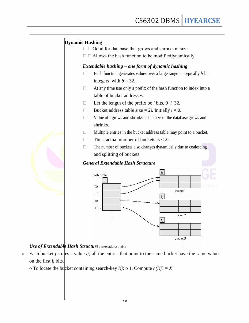
CS6302 DBMS IIYEARCSE
78
Dynamic Hashing
Good for database that grows and shrinks in size.
Allows the hash function to be modified dynamically.
Extendable hashing – one form of dynamic hashing
Hash function generates values over a large range — typically b-bit
integers, with b = 32.
At any time use only a prefix of the hash function to index into a
table of bucket addresses.
Let the length of the prefix be i bits, 0 i 32.
Bucket address table size = 2i. Initially i = 0.
Value of i grows and shrinks as the size of the database grows and
shrinks.
Multiple entries in the bucket address table may point to a bucket.
Thus, actual number of buckets is < 2i.
The number of buckets also changes dynamically due to coalescing
and splitting of buckets.
General Extendable Hash Structure Use of Extendable Hash Structure
o Each bucket j stores a value ij; all the entries that point to the same bucket have the same values
on the first ij bits. o To locate the bucket containing search-key Kj: o 1. Compute h(Kj) = X
CS6302 DBMS IIYEARCSE
79
o 2. Use the first i high order bits of X as a displacement into bucket
address table, and follow the pointer to appropriate bucket
o To insert a record with search-key value Kj
o follow same procedure as look-up and locate the bucket, say j.
o If there is room in the bucket j insert record in the bucket.
o Else the bucket must be split and insertion re-attempted. o Overflow buckets used instead in some cases.
Updates in Extendable Hash Structure
o To split a bucket j when inserting record with search-key value Kj: o If i > ij (more than one pointer to bucket j) o allocate a new bucket z, and set ij and iz to the old ij -+ 1.
o make the second half of the bucket address table entries pointing to j to point to z o remove and reinsert each record in bucket j.
o recompute new bucket for Kj and insert record in the bucket (fur-ther splitting is required if the
bucket is still full) o If i = ij (only one pointer to bucket j) o increment i and double the size of the bucket address table.
o replace each entry in the table by two entries that point to the same bucket. o recompute new bucket address table entry for Kj Now i > ij so use the first case above.
o When inserting a value, if the bucket is full after several splits (that is, i reaches some limit b)
create an overflow bucket instead of
splitting bucket entry table further. o To delete a key value, o locate it in its bucket and remove it.
o The bucket itself can be removed if it becomes empty (with appro-priate updates to the bucket
address table). o Coalescing of buckets can be done (can coalesce only with a ―buddy‖ bucket having same value
of ij and same ij –1 prefix, if it is present). o Decreasing bucket address table size is also possible.
o Note: decreasing bucket address table size is an expensive opera-tion and should be done only if
number of buckets becomes much smaller than the size of the table.
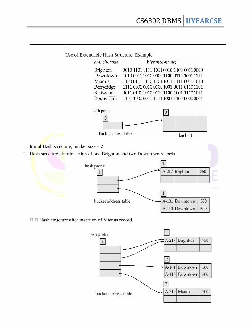
CS6302 DBMS IIYEARCSE
80
Use of Extendable Hash Structure: Example
Initial Hash structure, bucket size = 2
Hash structure after insertion of one Brighton and two Downtown records
Hash structure after insertion of Mianus record
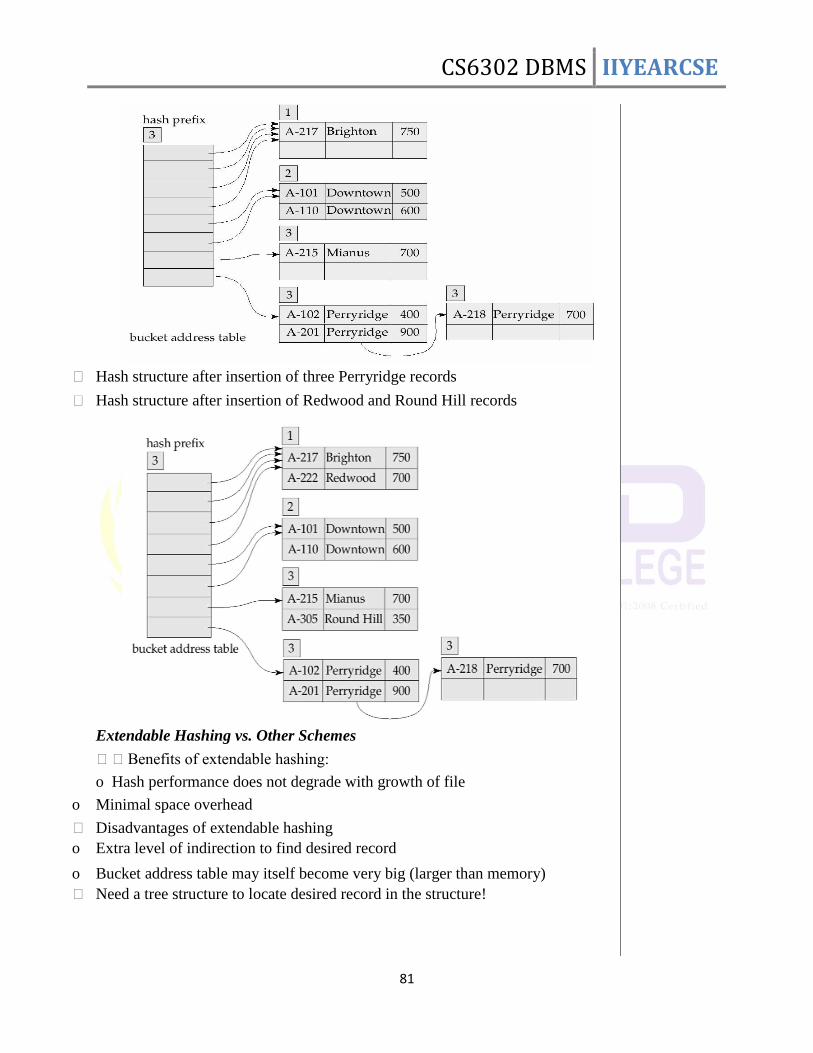
CS6302 DBMS IIYEARCSE
81
Hash structure after insertion of three Perryridge records
Hash structure after insertion of Redwood and Round Hill records
Extendable Hashing vs. Other Schemes Benefits of extendable hashing: o Hash performance does not degrade with growth of file
o Minimal space overhead
Disadvantages of extendable hashing o Extra level of indirection to find desired record
o Bucket address table may itself become very big (larger than memory) Need a tree structure to locate desired record in the structure!
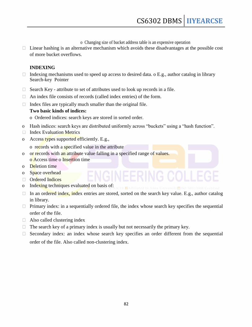
CS6302 DBMS IIYEARCSE
82
o Changing size of bucket address table is an expensive operation
Linear hashing is an alternative mechanism which avoids these disadvantages at the possible cost
of more bucket overflows.
INDEXING Indexing mechanisms used to speed up access to desired data. o E.g., author catalog in library
Search-key Pointer
Search Key - attribute to set of attributes used to look up records in a file.
An index file consists of records (called index entries) of the form.
Index files are typically much smaller than the original file. Two basic kinds of indices: o Ordered indices: search keys are stored in sorted order.
o Hash indices: search keys are distributed uniformly across ―buckets‖ using a ―hash function‖. Index Evaluation Metrics o Access types supported efficiently. E.g.,
o records with a specified value in the attribute
o or records with an attribute value falling in a specified range of values. o Access time o Insertion time
o Deletion time
o Space overhead
Ordered Indices o Indexing techniques evaluated on basis of:
In an ordered index, index entries are stored, sorted on the search key value. E.g., author catalog
in library.
Primary index: in a sequentially ordered file, the index whose search key specifies the sequential
order of the file.
Also called clustering index The search key of a primary index is usually but not necessarily the primary key.
Secondary index: an index whose search key specifies an order different from the sequential
order of the file. Also called non-clustering index.
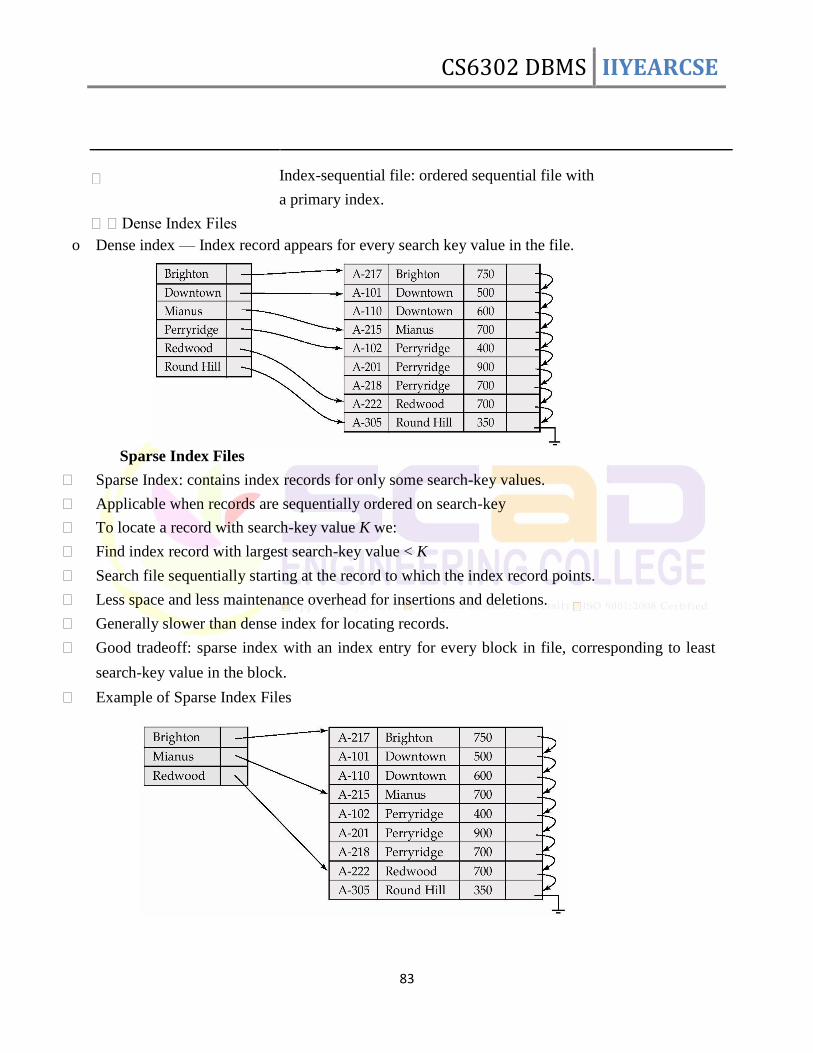
CS6302 DBMS IIYEARCSE
83
Index-sequential file: ordered sequential file with
a primary index.
Dense Index Files o Dense index — Index record appears for every search key value in the file.
Sparse Index Files
Sparse Index: contains index records for only some search-key values.
Applicable when records are sequentially ordered on search-key
To locate a record with search-key value K we:
Find index record with largest search-key value < K
Search file sequentially starting at the record to which the index record points.
Less space and less maintenance overhead for insertions and deletions.
Generally slower than dense index for locating records.
Good tradeoff: sparse index with an index entry for every block in file, corresponding to least
search-key value in the block.
Example of Sparse Index Files
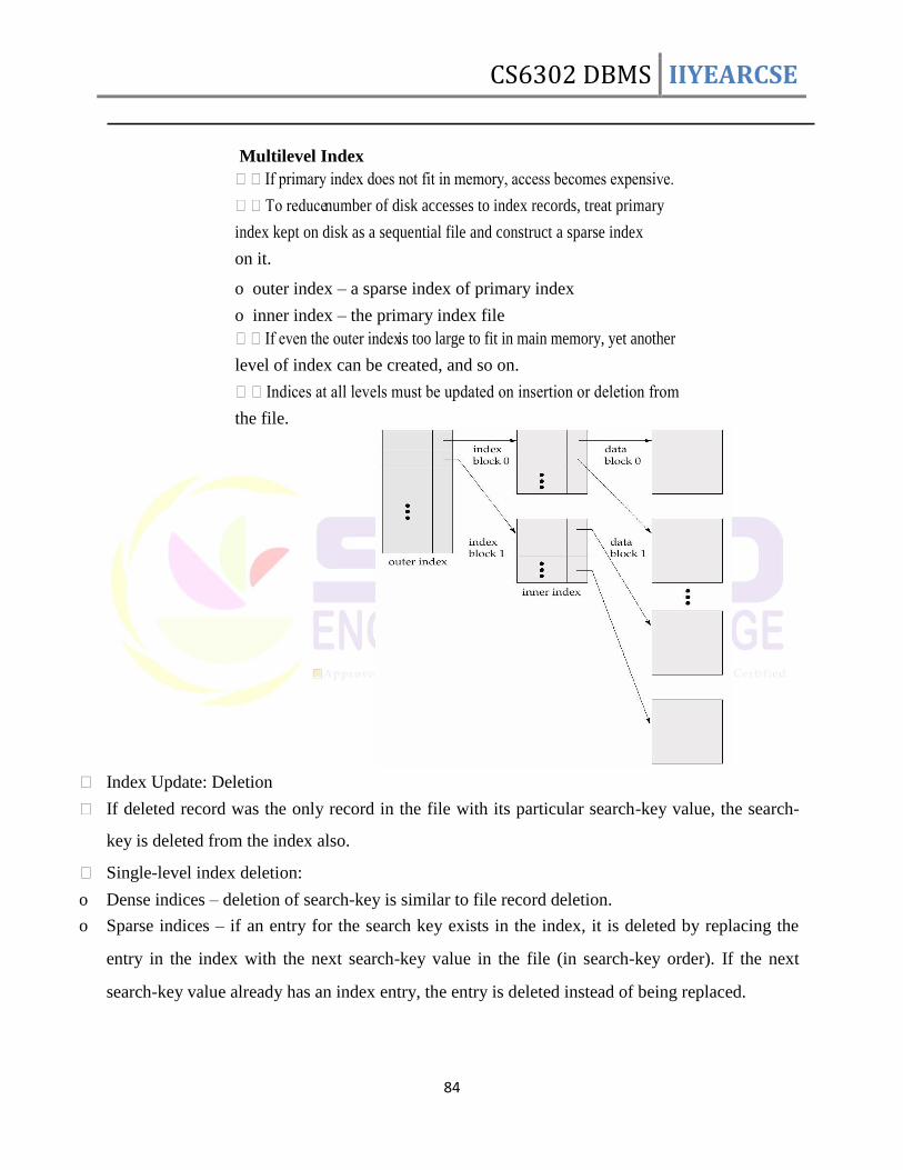
CS6302 DBMS IIYEARCSE
84
Multilevel Index
If primary index does not fit in memory, access becomes expensive.
To reduce number of disk accesses to index records, treat primary
index kept on disk as a sequential file and construct a sparse index
on it.
o outer index – a sparse index of primary index
o inner index – the primary index file
If even the outer index is too large to fit in main memory, yet another
level of index can be created, and so on.
Indices at all levels must be updated on insertion or deletion from
the file.
Index Update: Deletion
If deleted record was the only record in the file with its particular search-key value, the search-
key is deleted from the index also.
Single-level index deletion:
o Dense indices – deletion of search-key is similar to file record deletion.
o Sparse indices – if an entry for the search key exists in the index, it is deleted by replacing the
entry in the index with the next search-key value in the file (in search-key order). If the next
search-key value already has an index entry, the entry is deleted instead of being replaced.
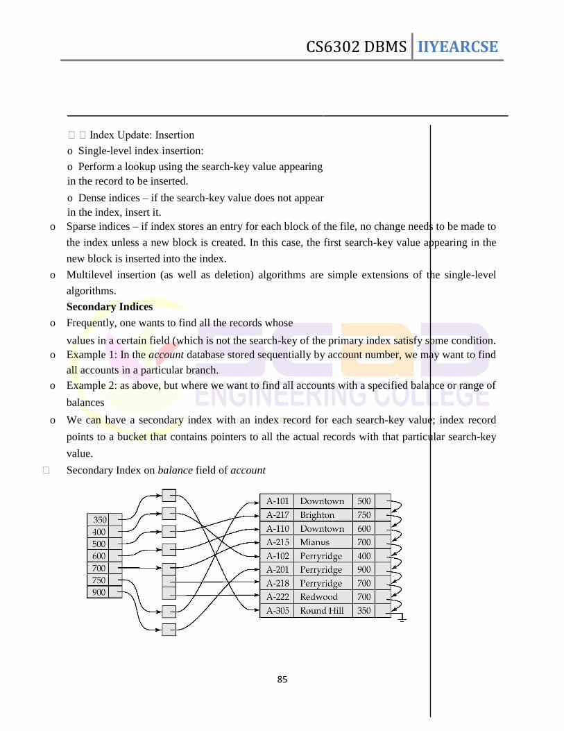
CS6302 DBMS IIYEARCSE
85
Index Update: Insertion
o Single-level index insertion:
o Perform a lookup using the search-key value appearing
in the record to be inserted.
o Dense indices – if the search-key value does not appear
in the index, insert it. o Sparse indices – if index stores an entry for each block of the file, no change needs to be made to
the index unless a new block is created. In this case, the first search-key value appearing in the
new block is inserted into the index.
o Multilevel insertion (as well as deletion) algorithms are simple extensions of the single-level
algorithms. Secondary Indices
o Frequently, one wants to find all the records whose values in a certain field (which is not the search-key of the primary index satisfy some condition.
o Example 1: In the account database stored sequentially by account number, we may want to find
all accounts in a particular branch.
o Example 2: as above, but where we want to find all accounts with a specified balance or range of
balances
o We can have a secondary index with an index record for each search-key value; index record
points to a bucket that contains pointers to all the actual records with that particular search-key
value.
Secondary Index on balance field of account

CS6302 DBMS IIYEARCSE
86
Primary and Secondary Indices Secondary indices have to be dense. Indices offer substantial benefits when searching for records.
When a file is modified, every index on the file must be updated, Updating indices imposes
overhead on database modification.
Sequential scan using primary index is efficient, but a sequential scan using a secondary index is
expensive.
each record access may fetch a new block from disk
Bitmap Indices
n Bitmap indices are a special type of index designed for efficient querying on multiple keys. n Records in a relation are assumed to be numbered sequentially from, say, 0
Given a number n it must be easy to retrieve record n
Particularly easy if records are of fixed size
n Applicable on attributes that take on a relatively small number of distinct values
E.g. gender, country, state, …
E.g. income-level (income broken up into a small number of levels such as 0-9999, 10000-
19999, 20000-50000, 50000- infinity) n A bitmap is simply an array of bits.
n In its simplest form a bitmap index on an attribute has a bitmap for each value of the attribute.
Bitmap has as many bits as records.
In a bitmap for value v, the bit for a record is 1 if the record has the value v for the attribute, and
is 0 otherwise.
n Bitmap indices are useful for queries on multiple attributes
Not particularly useful for single attribute queries
n Queries are answered using bitmap operations
Intersection (and)
Union (or)
Complementation (not)
n Each operation takes two bitmaps of the same size and applies the operation on corresponding
bits to get the result bitmap
Males with income level L1: 10010 AND 10100 = 10000
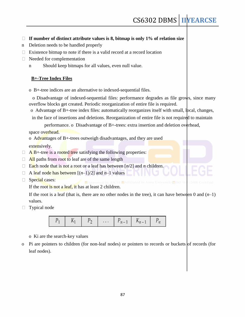
CS6302 DBMS IIYEARCSE
87
If number of distinct attribute values is 8, bitmap is only 1% of relation size
n Deletion needs to be handled properly
Existence bitmap to note if there is a valid record at a record location Needed for complementation
n Should keep bitmaps for all values, even null value.
B+-Tree Index Files
o B+-tree indices are an alternative to indexed-sequential files.
o Disadvantage of indexed-sequential files: performance degrades as file grows, since many
overflow blocks get created. Periodic reorganization of entire file is required. o Advantage of B+-tree index files: automatically reorganizes itself with small, local, changes,
in the face of insertions and deletions. Reorganization of entire file is not required to maintain
performance. o Disadvantage of B+-trees: extra insertion and deletion overhead,
space overhead. o Advantages of B+-trees outweigh disadvantages, and they are used extensively.
A B+-tree is a rooted tree satisfying the following properties:
All paths from root to leaf are of the same length Each node that is not a root or a leaf has between [n/2] and n children.
A leaf node has between [(n–1)/2] and n–1 values
Special cases:
If the root is not a leaf, it has at least 2 children.
If the root is a leaf (that is, there are no other nodes in the tree), it can have between 0 and (n–1)
values. Typical node
o Ki are the search-key values
o Pi are pointers to children (for non-leaf nodes) or pointers to records or buckets of records (for
leaf nodes).
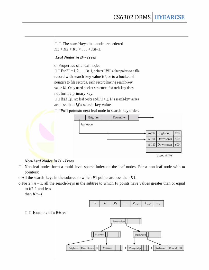
CS6302 DBMS IIYEARCSE
88
The search-keys in a node are ordered
K1 < K2 < K3 < . . . < Kn–1.
Leaf Nodes in B+-Trees
o Properties of a leaf node:
Fori= 1, 2, . . .,n–1, pointerPieither points to a file
record with search-key value Ki, or to a bucket of
pointers to file records, each record having search-key
value Ki. Only need bucket structure if search-key does
not form a primary key.
IfLi, Ljare leaf nodes andi<j, Li‘s search-key values
are less than Lj‘s search-key values.
Pnpoints to next leaf node in search-key order.
Non-Leaf Nodes in B+-Trees Non leaf nodes form a multi-level sparse index on the leaf nodes. For a non-leaf node with m
pointers: o All the search-keys in the subtree to which P1 points are less than K1. o For 2 i n – 1, all the search-keys in the subtree to which Pi points have values greater than or equal
to Ki–1 and less than Km–1. Example of a B+-tree
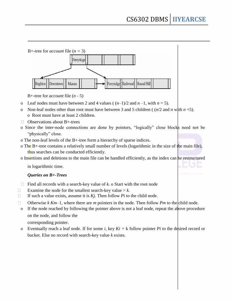
CS6302 DBMS IIYEARCSE
89
B+-tree for account file (n = 3) B+-tree for account file (n - 5)
o Leaf nodes must have between 2 and 4 values ( (n–1)/2 and n –1, with n = 5). o Non-leaf nodes other than root must have between 3 and 5 children ( (n/2 and n with n =5).
o Root must have at least 2 children.
Observations about B+-trees o Since the inter-node connections are done by pointers, ―logically‖ close blocks need not be
―physically‖ close.
o The non-leaf levels of the B+-tree form a hierarchy of sparse indices. o The B+-tree contains a relatively small number of levels (logarithmic in the size of the main file),
thus searches can be conducted efficiently. o Insertions and deletions to the main file can be handled efficiently, as the index can be restructured
in logarithmic time. Queries on B+-Trees
Find all records with a search-key value of k. o Start with the root node
Examine the node for the smallest search-key value > k. If such a value exists, assume it is Kj. Then follow Pi to the child node.
Otherwise k Km–1, where there are m pointers in the node. Then follow Pm to the child node. o If the node reached by following the pointer above is not a leaf node, repeat the above procedure
on the node, and follow the corresponding pointer.
o Eventually reach a leaf node. If for some i, key Ki = k follow pointer Pi to the desired record or
bucket. Else no record with search-key value k exists.
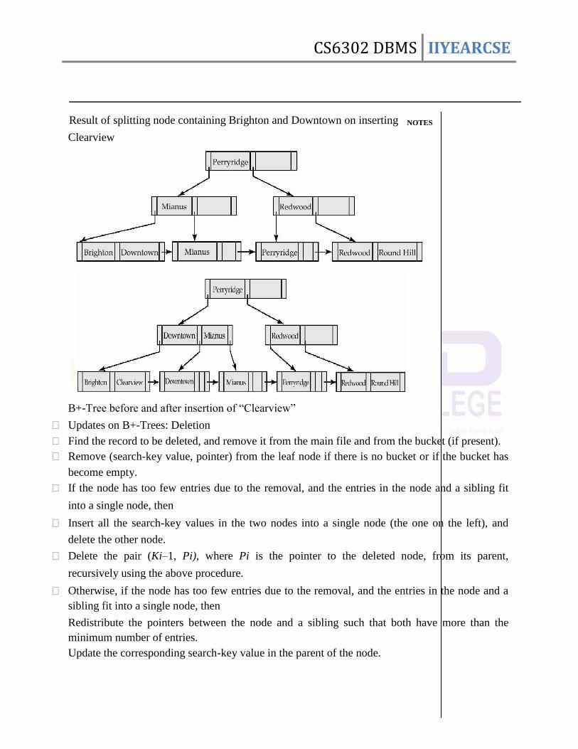
CS6302 DBMS IIYEARCSE
90
Result of splitting node containing Brighton and Downtown on inserting NOTES
Clearview B+-Tree before and after insertion of ―Clearview‖
Updates on B+-Trees: Deletion Find the record to be deleted, and remove it from the main file and from the bucket (if present). Remove (search-key value, pointer) from the leaf node if there is no bucket or if the bucket has
become empty.
If the node has too few entries due to the removal, and the entries in the node and a sibling fit
into a single node, then
Insert all the search-key values in the two nodes into a single node (the one on the left), and
delete the other node.
Delete the pair (Ki–1, Pi), where Pi is the pointer to the deleted node, from its parent,
recursively using the above procedure.
Otherwise, if the node has too few entries due to the removal, and the entries in the node and a
sibling fit into a single node, then
Redistribute the pointers between the node and a sibling such that both have more than the
minimum number of entries. Update the corresponding search-key value in the parent of the node.
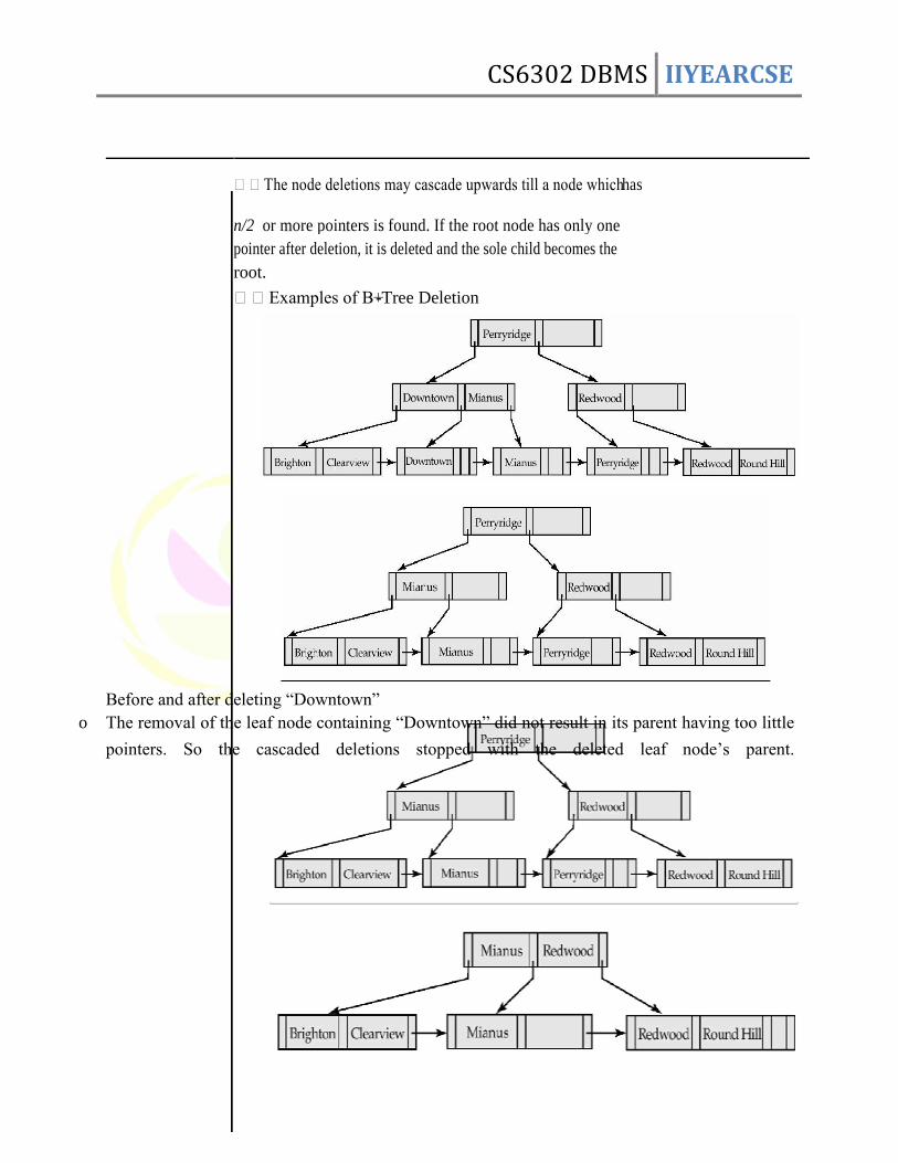
CS6302 DBMS IIYEARCSE
91
The node deletions may cascade upwards till a node which has
n/2 or more pointers is found. If the root node has only one
pointer after deletion, it is deleted and the sole child becomes the
root.
Examples of B+-Tree Deletion
Before and after deleting ―Downtown‖ o The removal of the leaf node containing ―Downtown‖ did not result in its parent having too little
pointers. So the cascaded deletions stopped with the deleted leaf node‘s parent.
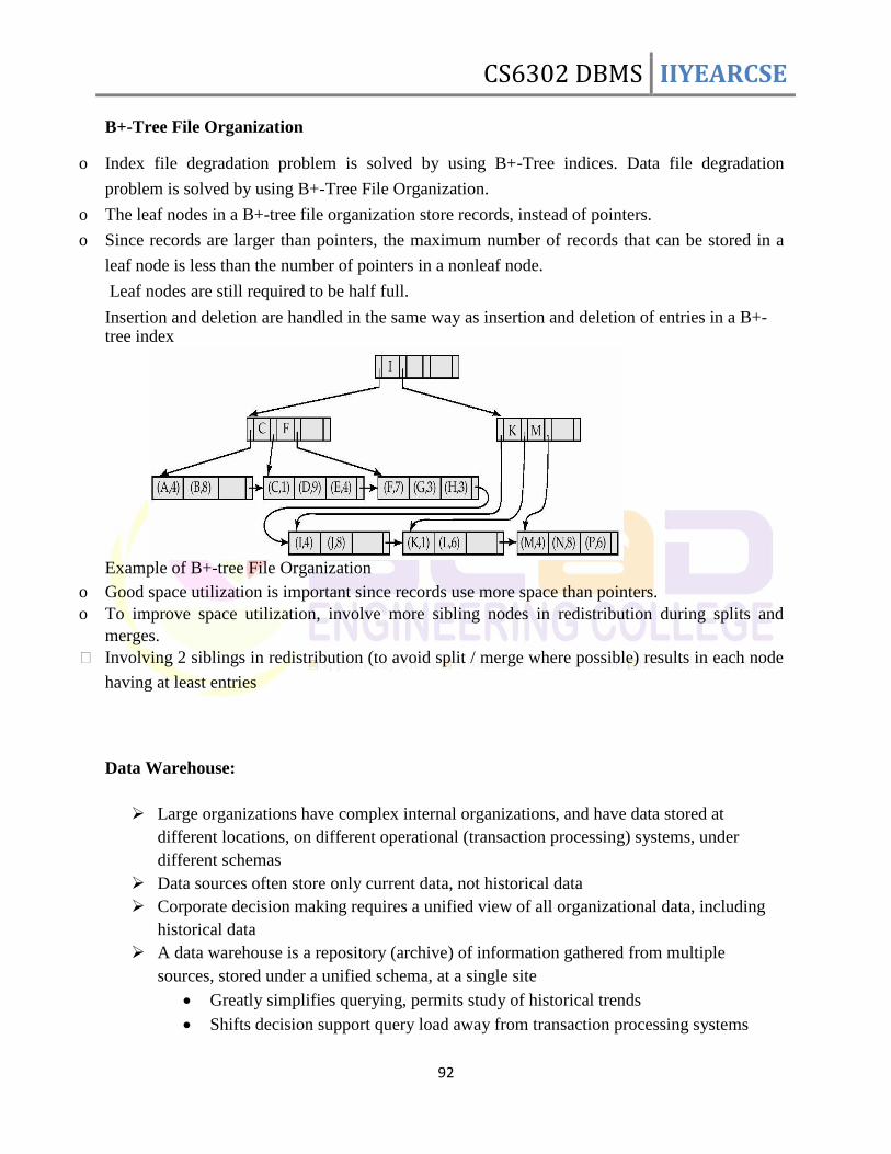
CS6302 DBMS IIYEARCSE
92
B+-Tree File Organization
o Index file degradation problem is solved by using B+-Tree indices. Data file degradation
problem is solved by using B+-Tree File Organization.
o The leaf nodes in a B+-tree file organization store records, instead of pointers.
o Since records are larger than pointers, the maximum number of records that can be stored in a
leaf node is less than the number of pointers in a nonleaf node. Leaf nodes are still required to be half full. Insertion and deletion are handled in the same way as insertion and deletion of entries in a B+-tree index
Example of B+-tree File Organization o Good space utilization is important since records use more space than pointers. o To improve space utilization, involve more sibling nodes in redistribution during splits and
merges.
Involving 2 siblings in redistribution (to avoid split / merge where possible) results in each node
having at least entries
Data Warehouse:
Large organizations have complex internal organizations, and have data stored at
different locations, on different operational (transaction processing) systems, under
different schemas
Data sources often store only current data, not historical data
Corporate decision making requires a unified view of all organizational data, including
historical data
A data warehouse is a repository (archive) of information gathered from multiple
sources, stored under a unified schema, at a single site
Greatly simplifies querying, permits study of historical trends
Shifts decision support query load away from transaction processing systems
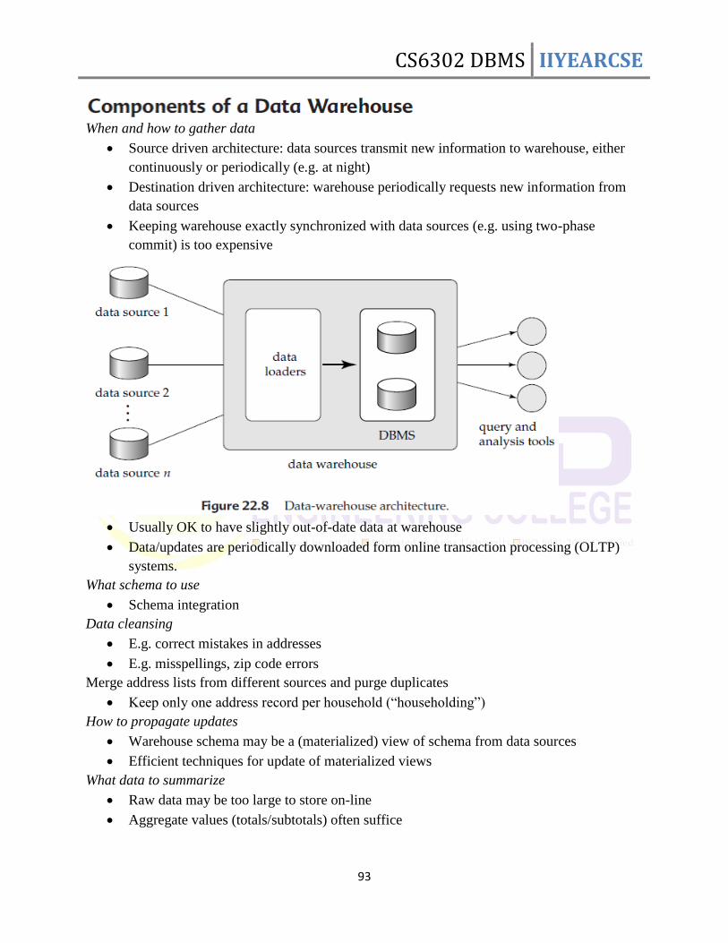
CS6302 DBMS IIYEARCSE
93
When and how to gather data
Source driven architecture: data sources transmit new information to warehouse, either
continuously or periodically (e.g. at night)
Destination driven architecture: warehouse periodically requests new information from
data sources
Keeping warehouse exactly synchronized with data sources (e.g. using two-phase
commit) is too expensive
Usually OK to have slightly out-of-date data at warehouse
Data/updates are periodically downloaded form online transaction processing (OLTP)
systems.
What schema to use
Schema integration
Data cleansing
E.g. correct mistakes in addresses
E.g. misspellings, zip code errors
Merge address lists from different sources and purge duplicates
Keep only one address record per household (―householding‖)
How to propagate updates
Warehouse schema may be a (materialized) view of schema from data sources
Efficient techniques for update of materialized views
What data to summarize
Raw data may be too large to store on-line
Aggregate values (totals/subtotals) often suffice
CS6302 DBMS IIYEARCSE
94
Queries on raw data can often be transformed by query optimizer to use aggregate
values.
Data Mining
Broadly speaking, data mining is the process of semi-automatically analyzing large
databases to find useful patterns.
Like knowledge discovery in artificial intelligence data mining discovers statistical rules
and patterns
Differs from machine learning in that it deals with large volumes of data stored primarily
on disk.
Some types of knowledge discovered from a database can be represented by a set of
rules. e.g.,: ―Young women with annual incomes greater than $50,000 are most likely to
buy sports cars‖.
Other types of knowledge represented by equations, or by prediction functions.
Some manual intervention is usually required
Pre-processing of data, choice of which type of pattern to find, postprocessing to
find novel patterns
Applications of Data Mining
Prediction based on past history
Predict if a credit card applicant poses a good credit risk, based on some
attributes (income, job type, age, ..) and past history
Predict if a customer is likely to switch brand loyalty
Predict if a customer is likely to respond to ―junk mail‖
Predict if a pattern of phone calling card usage is likely to be fraudulent
Some examples of prediction mechanisms:
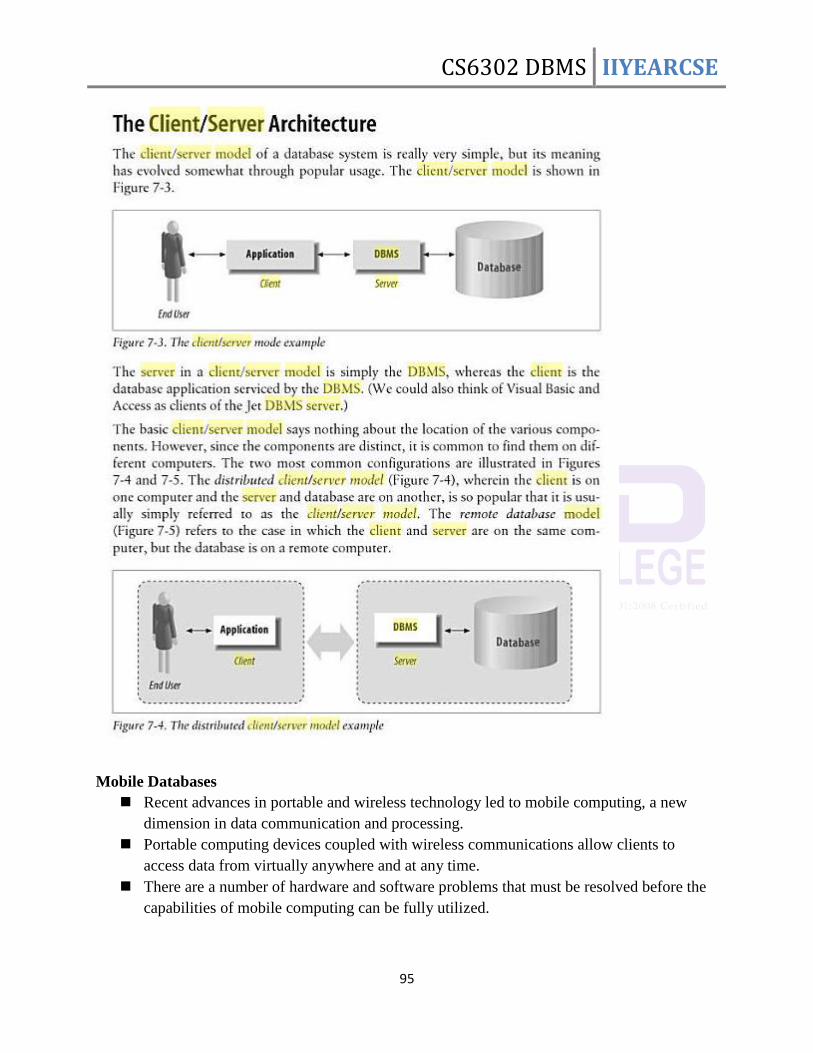
CS6302 DBMS IIYEARCSE
95
Mobile Databases
Recent advances in portable and wireless technology led to mobile computing, a new
dimension in data communication and processing.
Portable computing devices coupled with wireless communications allow clients to
access data from virtually anywhere and at any time.
There are a number of hardware and software problems that must be resolved before the
capabilities of mobile computing can be fully utilized.
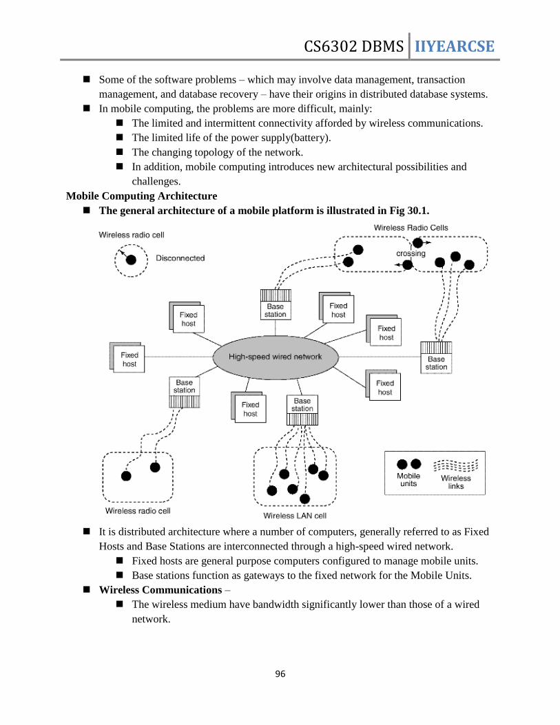
CS6302 DBMS IIYEARCSE
96
Some of the software problems – which may involve data management, transaction
management, and database recovery – have their origins in distributed database systems.
In mobile computing, the problems are more difficult, mainly:
The limited and intermittent connectivity afforded by wireless communications.
The limited life of the power supply(battery).
The changing topology of the network.
In addition, mobile computing introduces new architectural possibilities and
challenges.
Mobile Computing Architecture
The general architecture of a mobile platform is illustrated in Fig 30.1.
It is distributed architecture where a number of computers, generally referred to as Fixed
Hosts and Base Stations are interconnected through a high-speed wired network.
Fixed hosts are general purpose computers configured to manage mobile units.
Base stations function as gateways to the fixed network for the Mobile Units.
Wireless Communications –
The wireless medium have bandwidth significantly lower than those of a wired
network.
CS6302 DBMS IIYEARCSE
97
The current generation of wireless technology has data rates range from
the tens to hundreds of kilobits per second (2G cellular telephony) to tens
of megabits per second (wireless Ethernet, popularly known as WiFi).
Modern (wired) Ethernet, by comparison, provides data rates on the order
of hundreds of megabits per second.
The other characteristics distinguish wireless connectivity options:
interference,
locality of access,
range,
support for packet switching,
seamless roaming throughout a geographical region.
Some wireless networks, such as WiFi and Bluetooth, use unlicensed areas of the
frequency spectrum, which may cause interference with other appliances, such as
cordless telephones.
Modern wireless networks can transfer data in units called packets, that are used
in wired networks in order to conserve bandwidth.
Client/Network Relationships –
Mobile units can move freely in a geographic mobility domain, an area that is
circumscribed by wireless network coverage.
To manage entire mobility domain is divided into one or more smaller
domains, called cells, each of which is supported by at least one base
station.
Mobile units be unrestricted throughout the cells of domain, while
maintaining information access contiguity.
The communication architecture described earlier is designed to give the mobile
unit the impression that it is attached to a fixed network, emulating a traditional
client-server architecture.
Wireless communications, however, make other architectures possible. One
alternative is a mobile ad-hoc network (MANET), illustrated in 29.2.
In a MANET, co-located mobile units do not need to communicate via a fixed
network, but instead, form their own using cost-effective technologies such as
Bluetooth.
In a MANET, mobile units are responsible for routing their own data, effectively
acting as base stations as well as clients.
Moreover, they must be robust enough to handle changes in the network
topology, such as the arrival or departure of other mobile units.
MANET applications can be considered as peer-to-peer, meaning that a mobile
unit is simultaneously a client and a server.
Transaction processing and data consistency control become more
difficult since there is no central control in this architecture.
CS6302 DBMS IIYEARCSE
98
Resource discovery and data routing by mobile units make computing in a
MANET even more complicated.
Sample MANET applications are multi-user games, shared whiteboard,
distributed calendars, and battle information sharing.
Characteristics of Mobile Environments
The characteristics of mobile computing include:
Communication latency
Intermittent connectivity
Limited battery life
Changing client location
The server may not be able to reach a client.
A client may be unreachable because it is dozing – in an energy-conserving state
in which many subsystems are shut down – or because it is out of range of a base
station.
In either case, neither client nor server can reach the other, and
modifications must be made to the architecture in order to compensate for
this case.
Proxies for unreachable components are added to the architecture.
For a client (and symmetrically for a server), the proxy can cache updates
intended for the server.
Mobile computing poses challenges for servers as well as clients.
The latency involved in wireless communication makes scalability a problem.
Since latency due to wireless communications increases the time to
service each client request, the server can handle fewer clients.
One way servers relieve this problem is by broadcasting data whenever possible.
A server can simply broadcast data periodically.
Broadcast also reduces the load on the server, as clients do not have to maintain
active connections to it.
Client mobility also poses many data management challenges.
Servers must keep track of client locations in order to efficiently route messages
to them.
Client data should be stored in the network location that minimizes the traffic
necessary to access it.
The act of moving between cells must be transparent to the client.
The server must be able to gracefully divert the shipment of data from one base to
another, without the client noticing.
Client mobility also allows new applications that are location-based.
Spatial Database
Types of Spatial Data
Point Data
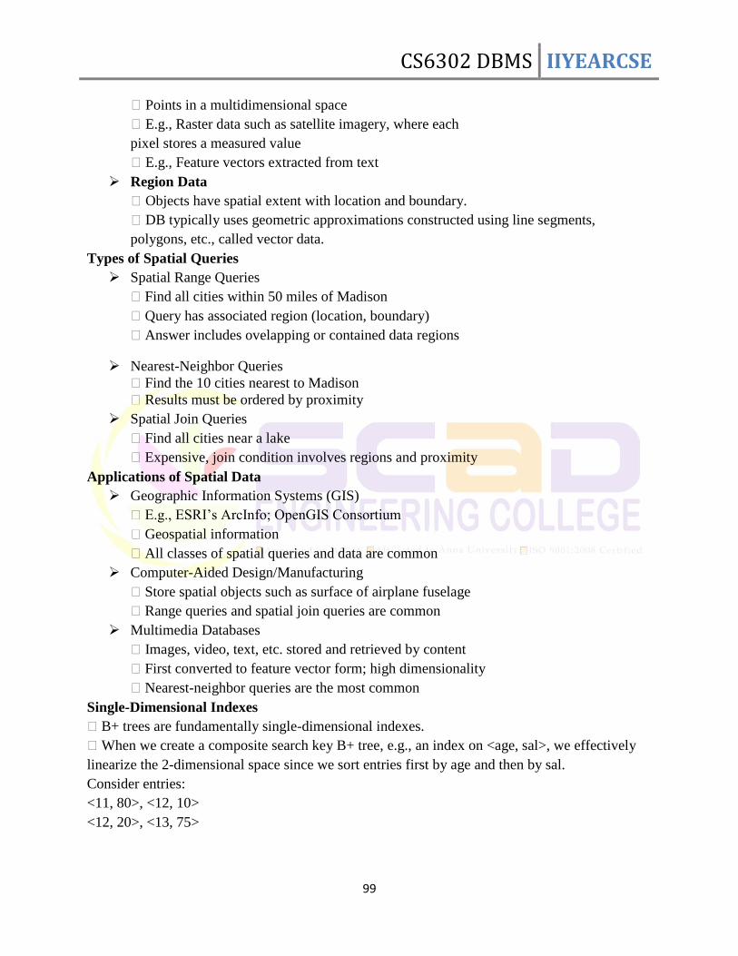
CS6302 DBMS IIYEARCSE
99
Points in a multidimensional space
E.g., Raster data such as satellite imagery, where each
pixel stores a measured value
E.g., Feature vectors extracted from text
Region Data
Objects have spatial extent with location and boundary.
DB typically uses geometric approximations constructed using line segments,
polygons, etc., called vector data.
Types of Spatial Queries
Spatial Range Queries
� Find all cities within 50 miles of Madison
� Query has associated region (location, boundary)
� Answer includes ovelapping or contained data regions
Nearest-Neighbor Queries
� Find the 10 cities nearest to Madison
� Results must be ordered by proximity
Spatial Join Queries
� Find all cities near a lake
� Expensive, join condition involves regions and proximity
Applications of Spatial Data
Geographic Information Systems (GIS)
� E.g., ESRI‘s ArcInfo; OpenGIS Consortium
� Geospatial information
� All classes of spatial queries and data are common
Computer-Aided Design/Manufacturing
� Store spatial objects such as surface of airplane fuselage
� Range queries and spatial join queries are common
Multimedia Databases
� Images, video, text, etc. stored and retrieved by content
� First converted to feature vector form; high dimensionality
� Nearest-neighbor queries are the most common
Single-Dimensional Indexes
� B+ trees are fundamentally single-dimensional indexes.
� When we create a composite search key B+ tree, e.g., an index on <age, sal>, we effectively
linearize the 2-dimensional space since we sort entries first by age and then by sal.
Consider entries:
<11, 80>, <12, 10>
<12, 20>, <13, 75>
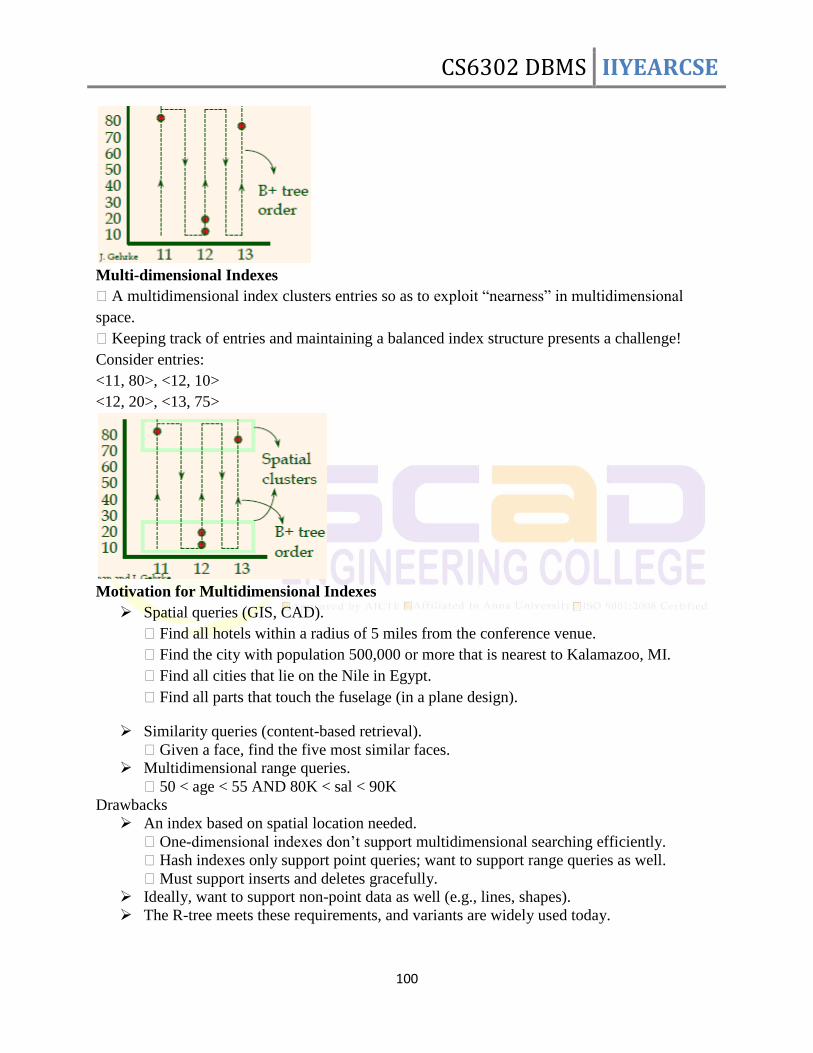
CS6302 DBMS IIYEARCSE
100
Multi-dimensional Indexes
� A multidimensional index clusters entries so as to exploit ―nearness‖ in multidimensional
space.
� Keeping track of entries and maintaining a balanced index structure presents a challenge!
Consider entries:
<11, 80>, <12, 10>
<12, 20>, <13, 75>
Motivation for Multidimensional Indexes
Spatial queries (GIS, CAD).
� Find all hotels within a radius of 5 miles from the conference venue.
� Find the city with population 500,000 or more that is nearest to Kalamazoo, MI.
� Find all cities that lie on the Nile in Egypt.
� Find all parts that touch the fuselage (in a plane design).
Similarity queries (content-based retrieval).
� Given a face, find the five most similar faces.
Multidimensional range queries.
� 50 < age < 55 AND 80K < sal < 90K
Drawbacks
An index based on spatial location needed.
� One-dimensional indexes don‘t support multidimensional searching efficiently.
� Hash indexes only support point queries; want to support range queries as well.
� Must support inserts and deletes gracefully.
Ideally, want to support non-point data as well (e.g., lines, shapes).
The R-tree meets these requirements, and variants are widely used today.
CS6302 DBMS IIYEARCSE
101
Multimedia databases
To provide such database functions as indexing and consistency, it is desirable to store
multimedia data in a database
� Rather than storing them outside the database, in a file system
The database must handle large object representation.
Similarity-based retrieval must be provided by special index structures.
Must provide guaranteed steady retrieval rates for continuous-media data.
Multimedia Data Formats
Store and transmit multimedia data in compressed form
� JPEG and GIF the most widely used formats for image data.
� MPEG standard for video data use commonalties among a sequence of frames to
achieve a greater degree of compression.
MPEG-1 quality comparable to VHS video tape.
� Stores a minute of 30-frame-per-second video and audio in approximately 12.5 MB
MPEG-2 designed for digital broadcast systems and digital video disks; negligible loss of
video quality.
� Compresses 1 minute of audio-video to approximately 17 MB.
Several alternatives of audio encoding
� MPEG-1 Layer 3 (MP3), RealAudio, WindowsMedia format, etc.
Continuous-Media Data
Most important types are video and audio data.
Characterized by high data volumes and real-time information-delivery requirements.
� Data must be delivered sufficiently fast that there are no gaps in the audio or video.
� Data must be delivered at a rate that does not cause overflow of system buffers.
� Synchronization among distinct data streams must be maintained
video of a person speaking must show lips moving synchronously with
the audio
Video Servers
Video-on-demand systems deliver video from central video servers, across a network, to
terminals
� must guarantee end-to-end delivery rates
Current video-on-demand servers are based on file systems; existing database systems do
not meet real-time response requirements.
Multimedia data are stored on several disks (RAID configuration), or on tertiary storage
for less frequently accessed data.
Head-end terminals - used to view multimedia data
� PCs or TVs attached to a small, inexpensive computer called a set-top box.
Similarity-Based Retrieval
Examples of similarity based retrieval
CS6302 DBMS IIYEARCSE
102
Pictorial data: Two pictures or images that are slightly different as represented in the
database may be considered the same by a user.
� e.g., identify similar designs for registering a new trademark.
Audio data: Speech-based user interfaces allow the user to give a command or identify a
data item by speaking.
� e.g., test user input against stored commands.
Handwritten data: Identify a handwritten data item or command stored in the database
UNIT V
ADVANCED TOPICS
ACCESS CONTROL Privacy in Oracle
• user gets a password and user name
• Privileges : – Connect : users can read and update tables (can‘t create) – Resource: create tables, grant privileges and control auditing – DBA: any table in complete DB
• user owns tables they create
• they grant other users privileges: – Select : retrieval – Insert : new rows – Update : existing rows – Delete : rows – Alter : column def.
CS6302 DBMS IIYEARCSE
103
– Index : on tables
• owner can offer GRANT to other users as well
• Users can get audits of:
– list of successful/unsuccessful attempts to access tables
– selective audit E.g. update only
– control level of detail reported
• DBA has this and logon, logoff oracle, grants/revolts privilege
• Audit is stored in the Data Dictionary. Integrity
The integrity of a database concerns
– consistency
– correctness
– validity
– accuracy
• that it should reflect real world
• i.e... it reflects the rules of the organization it models.
• rules = integrity rules or integrity
constraints examples
• accidental corruption of the DB,
• invalid PATIENT #
• non serializable schedules
• recovery manager not restoring DB correctly after failure Basic concepts
• trying to reflect in the DB rules which govern
organization E.g.:
INPATENT(patent#, name, DOB, address, sex,
gp) LABREQ (patent#, test-type, date, reqdr)
• E.g. rules
– lab. test can‘t be requested for non-existent PATIENT (insert to
labreq) (referential)
– every PATIENT must have unique patent number (relation)
– PATIENT numbers are integers in the range 1-99999. (domain)
CS6302 DBMS IIYEARCSE
104
• real-world rules = integrity constraints
• Implicit Constraints - relation, domain, referential - integral part of
Relational model
– Relational constraints - define relation and attributes supported
by all RDBMS
– Domain constraints - underlying domains on which attributes
defined
– Referential constraints - attribute from one table referencing
another
• Integrity subsystem: conceptually responsible for enforcing
constraints, violation + action
– monitor updates to the databases, multi user system this
can get expensive
• integrity constraints shared by all applications, stored in system
catalogue defined by data definition
Relation constraints
• how we define relations in SQL
• using CREATE we give relation name and define attributes
E.g. CREATE TABLE INPATIENT (PATIENT #, INTEGER, NOT NULL,
name, VARCHAR (20), NOT NULL, .......
gpn VARCHAR (20),
PRIMARY KEY PATIENT#); Domain constraints
• Domains are very important to the relational model
• through attributes defined over common domains that relationships
between tuples belonging to different relations can be defined.
• This also ensures consistency in typing.
E.g
CREATE TABLE (PATIENT# DOMAIN (PATIENT #) not
NULL, name DOMAIN (name) not
NULL,
sex DOMAIN
(sex), PRIMARY KEY PATIENT #);
CS6302 DBMS IIYEARCSE
105
CREATE DOMAIN PATIENT# INTEGER PATIENT# > 0
PATIENT# <10000;
CREATE DOMAIN sex CHAR (1) in (‗M‘, ‗F‘);
Referential integrity • refers to foreign keys
• consequences for updates and deletes
• 3 possibilities for
– RESTRICTED: disallow the update/deletion of primary keys as
long as their are foreign keys referencing that primary key.
– CASCADES: update/deletion of the primary key has a cascading
effect on all tuples whose foreign key references that primary
key, (and they too are deleted).
– NULLIFIES: update/deletion of the primary key results in the
referencing foreign keys being set to null.
FOREIGN KEY gpn REFERENCES gpname OF TABLE GPLIST NULLS ALLOWED DELETION NULLIFIES UPDATE CASCADES; . Explicit (semantic) constraints
• defined by SQL but not widely implemented
• E.g.. can‘t overdraw if you have a poor credit rating
ASSERT OVERDRAFT_CONSTRAINT ON customer,
account: account.balance >0 AND account.acc# =
CUSTOMER.cust# AND
CUSTOMER.credit_rating = ‗poor‘;
• Triggers DEFINE TRIGGER reord-constraint ON
STOCK noinstock < reordlevel ACTION ORDER_PROC (part#); Static and Dynamic Constraints
• State or Transaction constraints
CS6302 DBMS IIYEARCSE
106
• static refer to legal DB states
• dynamic refer to legitimate transactions of the DB form one state to
another ASSERT payrise-constraint ON UPDATE OF employee:
• Security can protect the database against unauthorized users.
• Integrity can protect it against authorized users
– Domain integrity rules: maintain correctness of attribute values in
relations
– Intra-relational Integrity: correctness of relationships among atts.
in same rel.
– Referential integrity: concerned with maintaining correctness and
consistency of relationships between relations.
Recovery and Concurrency
• closely bound to the idea of Transaction Processing.
• important in large multi-user centralized environment.
Authorization in SQL
• File systems identify certain access privileges on files, E.g., read, write, execute.
• In partial analogy, SQL identifies six access privileges on relations, of which the most important are:
1. SELECT = the right to query the relation.
2. INSERT = the right to insert tuples into the relation – may refer to
one attribute, in which case the privilege is to specify only one
column of the inserted tuple.
3. DELETE = the right to delete tuples from the relation.
4. UPDATE = the right to update tuples of the relation – may refer to
one attribute.
Granting Privileges
• You have all possible privileges to the relations you create.
• You may grant privileges to any user if you have those privileges ―with grant option.‖
u You have this option to your own relations.
Example 1. Here, Sally can query Sells and can change prices, but cannot pass
CS6302 DBMS IIYEARCSE
107
on this power:
GRANT SELECT ON Sells,
UPDATE(price) ON
Sells
TO sally
DISTRIBUTED DATABASES VS CONVENTIONAL DATABASES
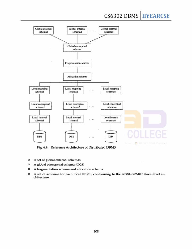
CS6302 DBMS IIYEARCSE
108
CS6302 DBMS IIYEARCSE
109
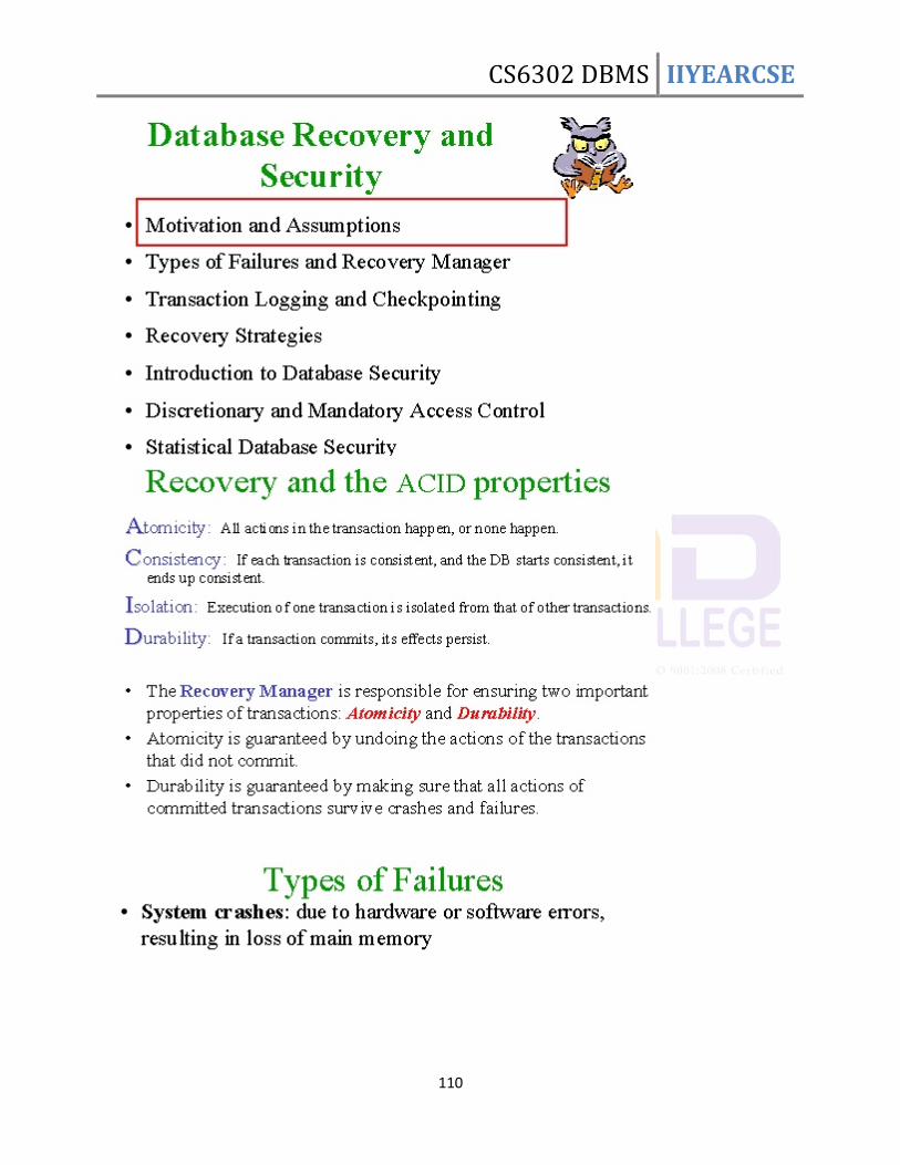
CS6302 DBMS IIYEARCSE
110
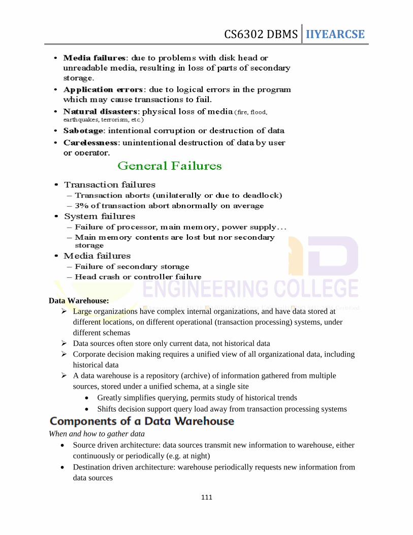
CS6302 DBMS IIYEARCSE
111
Data Warehouse:
Large organizations have complex internal organizations, and have data stored at
different locations, on different operational (transaction processing) systems, under
different schemas
Data sources often store only current data, not historical data
Corporate decision making requires a unified view of all organizational data, including
historical data
A data warehouse is a repository (archive) of information gathered from multiple
sources, stored under a unified schema, at a single site
Greatly simplifies querying, permits study of historical trends
Shifts decision support query load away from transaction processing systems
When and how to gather data
Source driven architecture: data sources transmit new information to warehouse, either
continuously or periodically (e.g. at night)
Destination driven architecture: warehouse periodically requests new information from
data sources
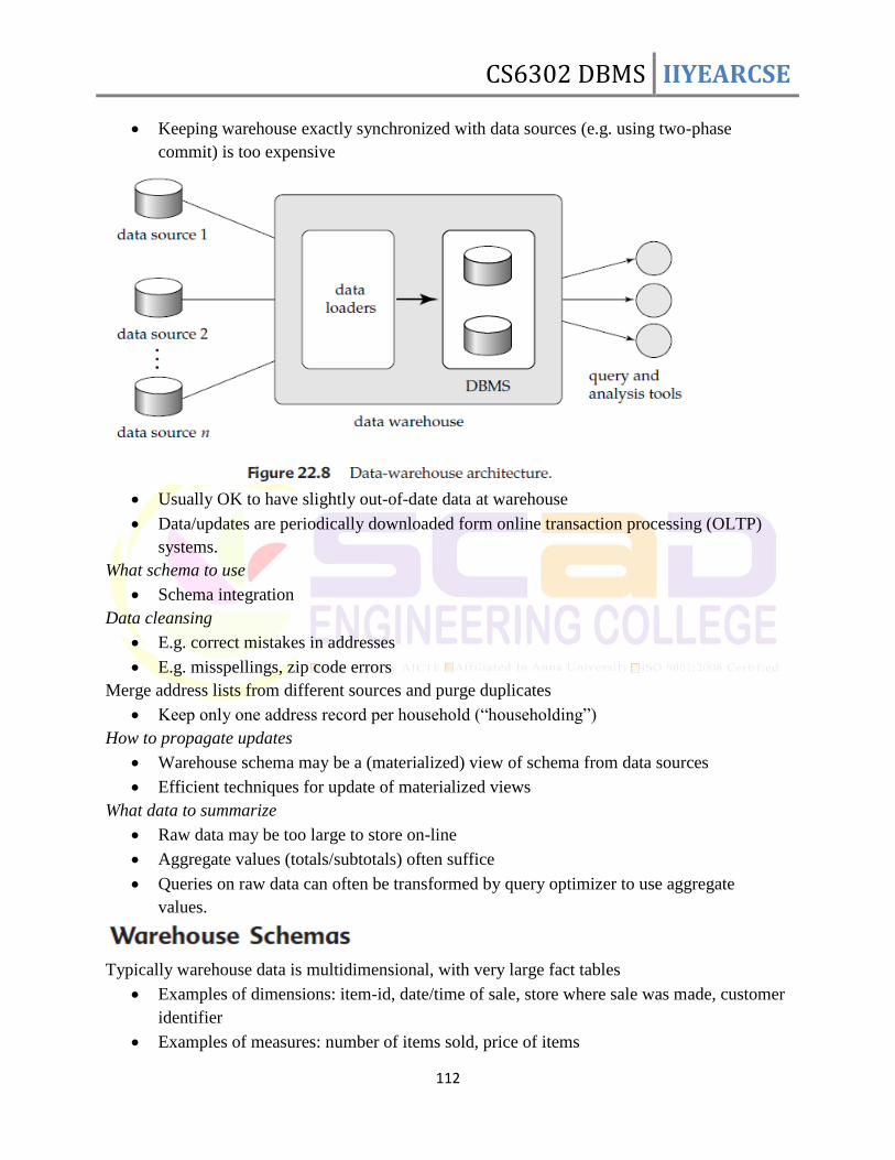
CS6302 DBMS IIYEARCSE
112
Keeping warehouse exactly synchronized with data sources (e.g. using two-phase
commit) is too expensive
Usually OK to have slightly out-of-date data at warehouse
Data/updates are periodically downloaded form online transaction processing (OLTP)
systems.
What schema to use
Schema integration
Data cleansing
E.g. correct mistakes in addresses
E.g. misspellings, zip code errors
Merge address lists from different sources and purge duplicates
Keep only one address record per household (―householding‖)
How to propagate updates
Warehouse schema may be a (materialized) view of schema from data sources
Efficient techniques for update of materialized views
What data to summarize
Raw data may be too large to store on-line
Aggregate values (totals/subtotals) often suffice
Queries on raw data can often be transformed by query optimizer to use aggregate
values.
Typically warehouse data is multidimensional, with very large fact tables
Examples of dimensions: item-id, date/time of sale, store where sale was made, customer
identifier
Examples of measures: number of items sold, price of items
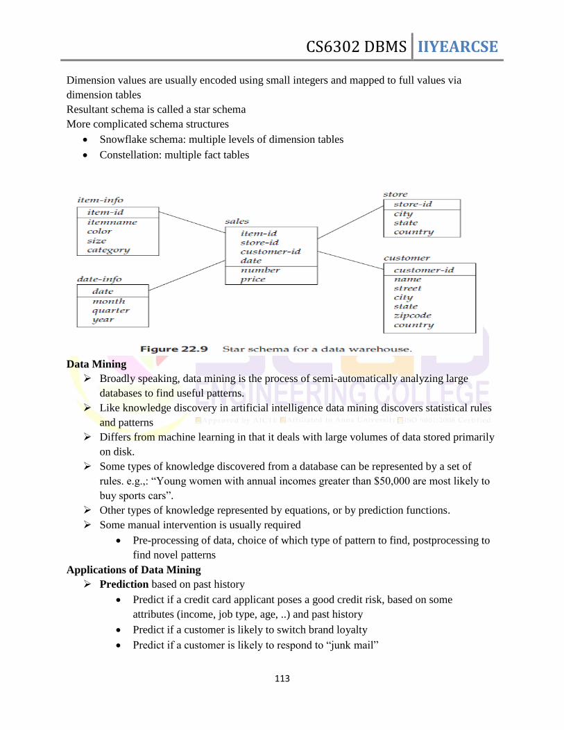
CS6302 DBMS IIYEARCSE
113
Dimension values are usually encoded using small integers and mapped to full values via
dimension tables
Resultant schema is called a star schema
More complicated schema structures
Snowflake schema: multiple levels of dimension tables
Constellation: multiple fact tables
Data Mining
Broadly speaking, data mining is the process of semi-automatically analyzing large
databases to find useful patterns.
Like knowledge discovery in artificial intelligence data mining discovers statistical rules
and patterns
Differs from machine learning in that it deals with large volumes of data stored primarily
on disk.
Some types of knowledge discovered from a database can be represented by a set of
rules. e.g.,: ―Young women with annual incomes greater than $50,000 are most likely to
buy sports cars‖.
Other types of knowledge represented by equations, or by prediction functions.
Some manual intervention is usually required
Pre-processing of data, choice of which type of pattern to find, postprocessing to
find novel patterns
Applications of Data Mining
Prediction based on past history
Predict if a credit card applicant poses a good credit risk, based on some
attributes (income, job type, age, ..) and past history
Predict if a customer is likely to switch brand loyalty
Predict if a customer is likely to respond to ―junk mail‖
CS6302 DBMS IIYEARCSE
114
Predict if a pattern of phone calling card usage is likely to be fraudulent
Some examples of prediction mechanisms:
Classification
Given a training set consisting of items belonging to different classes, and a new
item whose class is unknown, predict which class it belongs to.
Regression formulae
Given a set of parameter-value to function-result mappings for an unknown
function, predict the function-result for a new parameter-value
Descriptive Patterns
Associations
Find books that are often bought by the same customers. If a new customer buys
one such book, suggest that he buys the others too.
Other similar applications: camera accessories, clothes, etc.
Associations may also be used as a first step in detecting causation
E.g. association between exposure to chemical X and cancer, or new medicine
and cardiac problems
Clusters
E.g. typhoid cases were clustered in an area surrounding a contaminated well
Detection of clusters remains important in detecting epidemics
Classification Rules
Classification rules help assign new objects to a set of classes. E.g., given a new
automobile insurance applicant, should he or she be classified as low risk, medium risk
or high risk?
Classification rules for above example could use a variety of knowledge, such as
educational level of applicant, salary of applicant, age of applicant, etc.
person P, P.degree = masters and P.income > 75,000
P.credit = excellent
person P, P.degree = bachelors and
(P.income 25,000 and P.income 75,000)
P.credit = good
Rules are not necessarily exact: there may be some misclassifications
Classification rules can be compactly shown as a decision tree.
Decision Tree
Training set: a data sample in which the grouping for each tuple is already known.
Consider credit risk example: Suppose degree is chosen to partition the data at the root.
Since degree has a small number of possible values, one child is created for each
value.
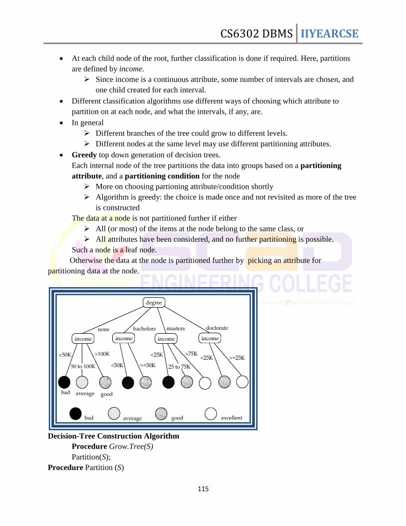
CS6302 DBMS IIYEARCSE
115
At each child node of the root, further classification is done if required. Here, partitions
are defined by income.
Since income is a continuous attribute, some number of intervals are chosen, and
one child created for each interval.
Different classification algorithms use different ways of choosing which attribute to
partition on at each node, and what the intervals, if any, are.
In general
Different branches of the tree could grow to different levels.
Different nodes at the same level may use different partitioning attributes.
Greedy top down generation of decision trees.
Each internal node of the tree partitions the data into groups based on a partitioning
attribute, and a partitioning condition for the node
More on choosing partioning attribute/condition shortly
Algorithm is greedy: the choice is made once and not revisited as more of the tree
is constructed
The data at a node is not partitioned further if either
All (or most) of the items at the node belong to the same class, or
All attributes have been considered, and no further partitioning is possible.
Such a node is a leaf node.
Otherwise the data at the node is partitioned further by picking an attribute for
partitioning data at the node.
Decision-Tree Construction Algorithm
Procedure Grow.Tree(S)
Partition(S);
Procedure Partition (S)
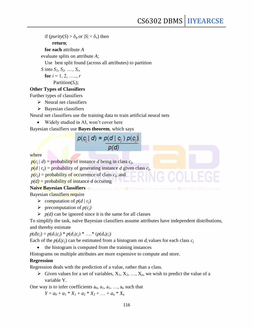
CS6302 DBMS IIYEARCSE
116
if (purity(S) > p or |S| < s) then
return;
for each attribute A
evaluate splits on attribute A;
Use best split found (across all attributes) to partition
S into S1, S2, …., Sr,
for i = 1, 2, ….., r
Partition(Si);
Other Types of Classifiers
Further types of classifiers
Neural net classifiers
Bayesian classifiers
Neural net classifiers use the training data to train artificial neural nets
Widely studied in AI, won‘t cover here
Bayesian classifiers use Bayes theorem, which says
where
p(cj | d) = probability of instance d being in class cj,
p(d | cj) = probability of generating instance d given class cj,
p(cj) = probability of occurrence of class cj, and
p(d) = probability of instance d occuring
Naive Bayesian Classifiers
Bayesian classifiers require
computation of p(d | cj)
precomputation of p(cj)
p(d) can be ignored since it is the same for all classes
To simplify the task, naïve Bayesian classifiers assume attributes have independent distributions,
and thereby estimate
p(d|cj) = p(d1|cj) * p(d2|cj) * ….* (p(dn|cj)
Each of the p(di|cj) can be estimated from a histogram on di values for each class cj
the histogram is computed from the training instances
Histograms on multiple attributes are more expensive to compute and store.
Regression
Regression deals with the prediction of a value, rather than a class.
Given values for a set of variables, X1, X2, …, Xn, we wish to predict the value of a
variable Y.
One way is to infer coefficients a0, a1, a1, …, an such that
Y = a0 + a1 * X1 + a2 * X2 + … + an * Xn
CS6302 DBMS IIYEARCSE
117
Finding such a linear polynomial is called linear regression.
In general, the process of finding a curve that fits the data is also called curve fitting.
The fit may only be approximate
because of noise in the data, or
because the relationship is not exactly a polynomial
Regression aims to find coefficients that give the best possible fit.
Association Rules
Retail shops are often interested in associations between different items that people buy.
Someone who buys bread is quite likely also to buy milk
A person who bought the book Database System Concepts is quite likely also to buy the
book Operating System Concepts.
Associations information can be used in several ways.
E.g. when a customer buys a particular book, an online shop may suggest associated
books.
Association rules:
bread milk DB-Concepts, OS-Concepts Networks
Left hand side: antecedent, right hand side: consequent
An association rule must have an associated population; the population consists of a set of
instances E.g. each transaction (sale) at a shop is an instance, and the set of all transactions is the
population.
Rules have an associated support, as well as an associated confidence.
Support is a measure of what fraction of the population satisfies both the antecedent and the
consequent of the rule.
E.g. suppose only 0.001 percent of all purchases include milk and screwdrivers. The support for
the rule is milk screwdrivers is low.
We usually want rules with a reasonably high support
Rules with low support are usually not very useful
Confidence is a measure of how often the consequent is true when the antecedent is true.
E.g. the rule bread milk has a confidence of 80 percent if 80 percent of the purchases that
include bread also include milk.
Usually want rules with reasonably large confidence.
Finding Association Rule
We are generally only interested in association rules with reasonably high support (e.g. support
of 2% or greater)
Naïve algorithm
1. Consider all possible sets of relevant items.
2. For each set find its support (i.e. count how many transactions purchase all items
in the set).
Large itemsets: sets with sufficiently high support
3. Use large itemsets to generate association rules.

CS6302 DBMS IIYEARCSE
118
From itemset A generate the rule A - {b} b for each b A.
Support of rule = support (A).
Confidence of rule = support (A ) / support (A - {b})
Other Types of Associations
Basic association rules have several limitations
Deviations from the expected probability are more interesting
E.g. if many people purchase bread, and many people purchase cereal, quite a few would be
expected to purchase both (prob1 * prob2)
We are interested in positive as well as negative correlations between sets of items
Positive correlation: co-occurrence is higher than predicted
Negative correlation: co-occurrence is lower than predicted
Sequence associations/correlations
E.g. whenever bonds go up, stock prices go down in 2 days
Deviations from temporal patterns
E.g. deviation from a steady growth
E.g. sales of winter wear go down in summer
Not surprising, part of a known pattern.
Look for deviation from value predicted using past patterns
Clustering
Clustering: Intuitively, finding clusters of points in the given data such that similar points
lie in the same cluster
Can be formalized using distance metrics in several ways
E.g. Group points into k sets (for a given k) such that the average distance of points from
the centroid of their assigned group is minimized
Centroid: point defined by taking average of coordinates in each dimension.
Another metric: minimize average distance between every pair of points in a cluster
Has been studied extensively in statistics, but on small data sets
Data mining systems aim at clustering techniques that can handle very large data sets
E.g. the Birch clustering algorithm (more shortly)
Hierarchical Clustering
Example from biological classification
Other examples: Internet directory systems (e.g. Yahoo, more on this later)
Agglomerative clustering algorithms
Build small clusters, then cluster small clusters into bigger clusters, and so on
Divisive clustering algorithms
Start with all items in a single cluster, repeatedly refine (break) clusters into smaller ones.
OBJECT ORIENTED DATABASE
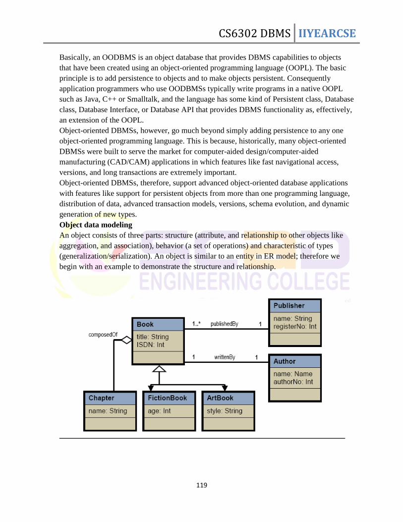
CS6302 DBMS IIYEARCSE
119
Basically, an OODBMS is an object database that provides DBMS capabilities to objects
that have been created using an object-oriented programming language (OOPL). The basic
principle is to add persistence to objects and to make objects persistent. Consequently
application programmers who use OODBMSs typically write programs in a native OOPL
such as Java, C++ or Smalltalk, and the language has some kind of Persistent class, Database
class, Database Interface, or Database API that provides DBMS functionality as, effectively,
an extension of the OOPL.
Object-oriented DBMSs, however, go much beyond simply adding persistence to any one
object-oriented programming language. This is because, historically, many object-oriented
DBMSs were built to serve the market for computer-aided design/computer-aided
manufacturing (CAD/CAM) applications in which features like fast navigational access,
versions, and long transactions are extremely important.
Object-oriented DBMSs, therefore, support advanced object-oriented database applications
with features like support for persistent objects from more than one programming language,
distribution of data, advanced transaction models, versions, schema evolution, and dynamic
generation of new types.
Object data modeling
An object consists of three parts: structure (attribute, and relationship to other objects like
aggregation, and association), behavior (a set of operations) and characteristic of types
(generalization/serialization). An object is similar to an entity in ER model; therefore we
begin with an example to demonstrate the structure and relationship.
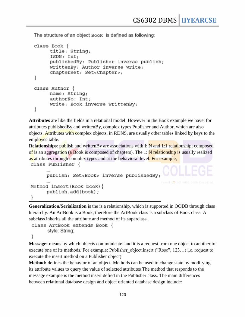
CS6302 DBMS IIYEARCSE
120
Attributes are like the fields in a relational model. However in the Book example we have, for
attributes publishedBy and writtenBy, complex types Publisher and Author, which are also
objects. Attributes with complex objects, in RDNS, are usually other tables linked by keys to the
employee table. Relationships: publish and writtenBy are associations with I: N and 1:1 relationship; composed
of is an aggregation (a Book is composed of chapters). The 1: N relationship is usually realized
as attributes through complex types and at the behavioral level. For example,
Generalization/Serialization is the is a relationship, which is supported in OODB through class
hierarchy. An ArtBook is a Book, therefore the ArtBook class is a subclass of Book class. A
subclass inherits all the attribute and method of its superclass.
Message: means by which objects communicate, and it is a request from one object to another to
execute one of its methods. For example: Publisher_object.insert (‖Rose‖, 123…) i.e. request to
execute the insert method on a Publisher object) Method: defines the behavior of an object. Methods can be used to change state by modifying
its attribute values to query the value of selected attributes The method that responds to the
message example is the method insert defied in the Publisher class. The main differences
between relational database design and object oriented database design include:
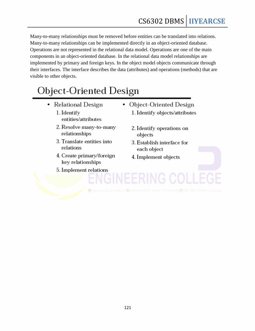
CS6302 DBMS IIYEARCSE
121
Many-to-many relationships must be removed before entities can be translated into relations.
Many-to-many relationships can be implemented directly in an object-oriented database.
Operations are not represented in the relational data model. Operations are one of the main
components in an object-oriented database. In the relational data model relationships are
implemented by primary and foreign keys. In the object model objects communicate through
their interfaces. The interface describes the data (attributes) and operations (methods) that are
visible to other objects.