Embed Size (px)
DESCRIPTION
algorithm
Citation preview
1
Streaming Algorithms
CS6234 – Advanced AlgorithmsNARMADA SAMBATURU
SUBHASREE BASUALOK KUMAR KESHRI
RAJIV RATN SHAHVENKATA KIRAN YEDUGUNDLA
VU VINH AN
2
Overview
• Introduction to Streaming Algorithms • Sampling Techniques • Sketching Techniques
Break• Counting Distinct Numbers• Q&A
3
Overview
• Introduction to Streaming Algorithms • Sampling Techniques • Sketching Techniques
Break• Counting Distinct Numbers• Q&A
4
What are Streaming algorithms?
• Algorithms for processing data streams• Input is presented as a sequence of items• Can be examined in only a few passes (typically just
one)• Limited working memory
5
Same as Online algorithms?
• Similarities decisions to be made before all data are available limited memory
• Differences Streaming algorithms – can defer action until a group of
points arrive Online algorithms - take action as soon as each point
arrives
6
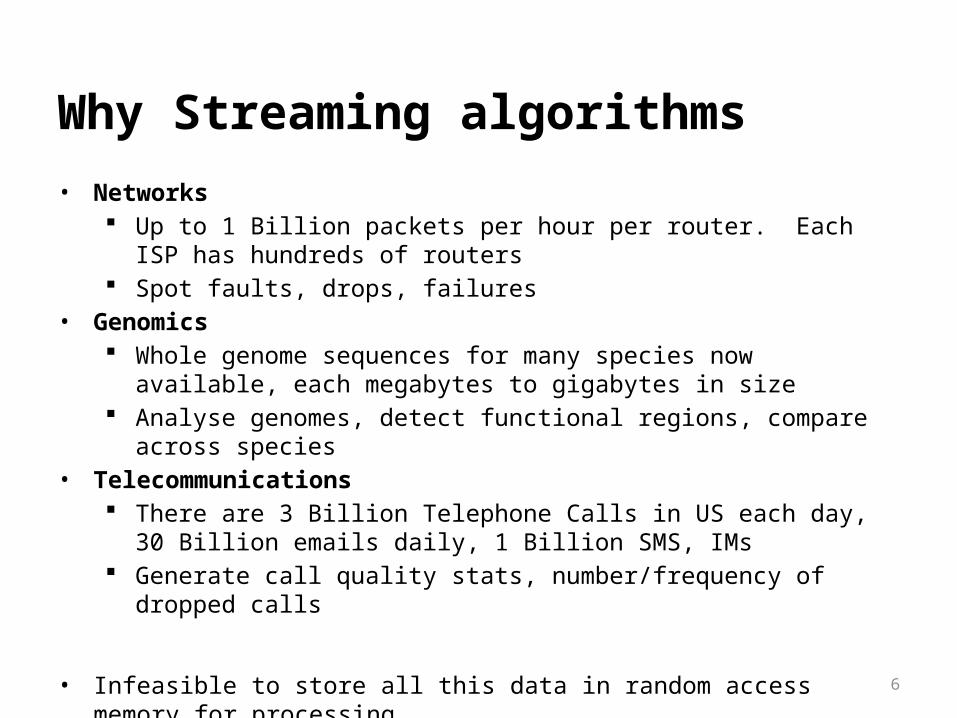
Why Streaming algorithms• Networks
Up to 1 Billion packets per hour per router. Each ISP has hundreds of routers Spot faults, drops, failures
• Genomics Whole genome sequences for many species now available, each megabytes to
gigabytes in size Analyse genomes, detect functional regions, compare across species
• Telecommunications There are 3 Billion Telephone Calls in US each day, 30 Billion emails daily, 1
Billion SMS, IMs Generate call quality stats, number/frequency of dropped calls
• Infeasible to store all this data in random access memory for processing.• Solution – process the data as a stream – streaming algorithms
7
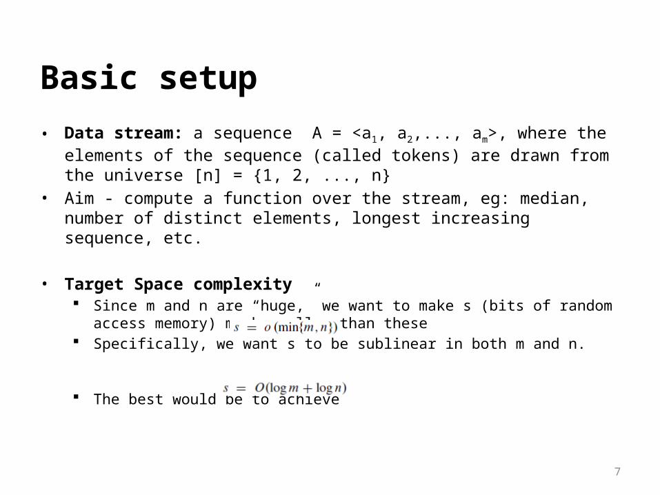
Basic setup• Data stream: a sequence A = <a1, a2,..., am>, where the elements of the sequence
(called tokens) are drawn from the universe [n] = {1, 2, ..., n}�• Aim - compute a function over the stream, eg: median, number of distinct
elements, longest increasing sequence, etc.
• Target Space complexity Since m and n are “huge,” we want to make s (bits of random access memory) much
smaller than these Specifically, we want s to be sublinear in both m and n.
The best would be to achieve
8
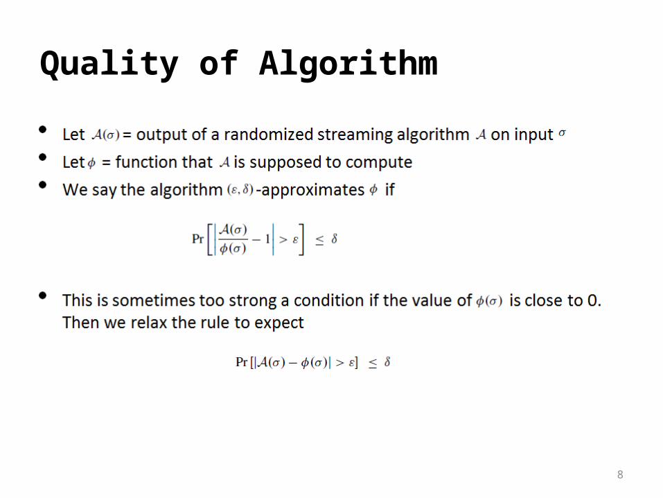
Quality of Algorithm

9
Streaming Models - Cash Register Model• Time-Series Model
Only x-th update is processed i.e., A[x] = c[x]
• Cash-Register Model: Arrivals-Only Streamsc[x] is always > 0 Typically, c[x]=1
• Example: <x, 3>, <y, 2>, <x, 2> encodes the arrival of 3 copies of item x, 2 copies of y, 2 copies of x.Could represent, packets in a network, power usage

10
Streaming Models – Turnstile Model• Turnstile Model: Arrivals and Departures
Most general streaming modelc[x] can be >0 or <0
• Example: <x, 3>, <y,2>, <x, -2> encodes final state of <x, 1>, <y, 2>.Can represent fluctuating quantities, or measure differences between two distributions
11
Overview
• Introduction to Streaming Algorithms • Sampling Techniques • Sketching Techniques• Break• Counting Distinct Numbers• Q&A

12
Sampling• Idea
A small random sample S of the data is often enough to represent all the data• Example
To compute median packet sizeSample some packetsPresent median size of sampled packets as true median
• ChallengeDon’t know how long the stream is
13
Reservoir Sampling - Idea
• We have a reservoir that can contain k samples• Initially accept every incoming sample till reservoir fills up• After reservoir is full, accept sample with probability
• This means as long as our reservoir has space, we sample every item
• Then we replace items in our reservoir with gradually decreasing probability

Reservoir Sampling - Algorithm

15
Probability Calculations

16
Probability of any element to be included at round t
Observation:Hence even though at the beginning a lot of elements get replaced, with the increase in the stream size, the probability of a new record evicting the old one drops.
• Let us consider a time t > N.• Let the number of elements that has arrived till now
be Nt
• Since at each round, all the elements have equal probabilities, the probability of any element being included in the sample is N/ Nt
17
Probability of any element to be chosen for the final Sample
• Let the final stream be of size NT • Claim: The probability of any element to be in the sample is
N/ NT

18
Probability of survival of the initial N elements• Let us choose any particular element out of ourinitial elements.( say)• The eviction tournament starts after the arrival of the element• Probability that element is chosen is • Probability that ifelement is chosen by evicting is • Hence probability ofbeing evicted in this case is
• Probability that survives
• Similarly the case eN survives when (N+2)nd element arrives = (N+1)/ (N+2)
• The probability of eN surviving two new records
= (N/(N+1)) X ((N+1)/ (N+2))• The probability of eN surviving till the end
= (N/(N+1)) X ((N+1)/ (N+2)) X ……. X ((NT -1)/ NT) = N/ NT
19
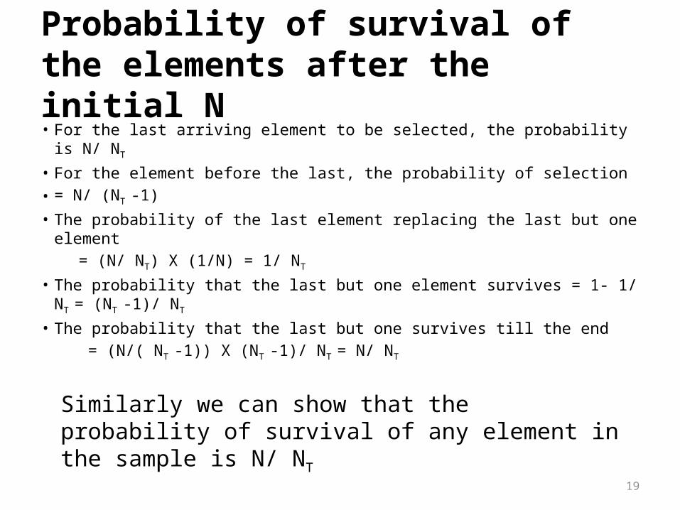
Probability of survival of the elements after the initial N• For the last arriving element to be selected, the probability is N/ NT
• For the element before the last, the probability of selection • = N/ (NT -1)• The probability of the last element replacing the last but one element = (N/ NT) X (1/N) = 1/ NT
• The probability that the last but one element survives = 1- 1/ NT = (NT -1)/ NT
• The probability that the last but one survives till the end = (N/( NT -1)) X (NT -1)/ NT = N/ NT
Similarly we can show that the probability of survival of any element in the sample is N/ NT

20
Calculating the Maximum Reservoir Size

21
Some Observations• Initially the reservoir contains N elements• Hence the size of the reservoir space is also N• New records are added to the reservoir only when it will replace any
element present previously in the reservoir. • If it is not replacing any element, then it is not added to the reservoir
space and we move on to the next element. • However we find that when an element is evicted from the reservoir, it
still exists in the reservoir storage space. • The position in the array that held its pointer, now holds some other
element’s pointer. But the element is still present in the reservoir space
• Hence the total number of elements in the reservoir space at any particular time ≥ N.
22
Maximum Size of the Reservoir
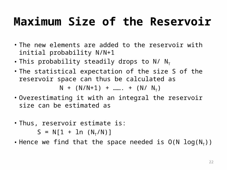
• The new elements are added to the reservoir with initial probability N/N+1
• This probability steadily drops to N/ NT
• The statistical expectation of the size S of the reservoir space can thus be calculated as
N + (N/N+1) + ……. + (N/ NT)• Overestimating it with an integral the reservoir size can be estimated
as
• Thus, reservoir estimate is: S = N[1 + ln (NT/N)]
• Hence we find that the space needed is O(N log(NT))

23
Priority Sample for Sliding Window

24
Reservoir Sampling Vs Sliding Window
• Works well when we have only inserts into a sample• The first element in the data stream can be retained in
the final sample • It does not consider the expiry of any record
Reservoir Sampling
Sliding Window
• Works well when we need to consider “timeliness” of the data• Data is considered to be expired after a certain time interval • “Sliding window” in essence is such a random sample of fixed
size (say k) “moving” over the most recent elements in the data stream

25
Types of Sliding Window
• Sequence-based
-- they are windows of size k moving over the k mist recently arrived data. Example being chain-sample algorithm
• Time-stamp based
-- windows of duration t consist of elements whose arrival timestamp is within a time interval t of the current time. Example being Priority Sample for Sliding Window
26
Principles of the Priority Sampling algorithm
• As each element arrives, it is assigned a randomly-chosen priority between 0 and 1
• An element is ineligible if there is another element with a later timestamp and higher priority
• The element selected for inclusion in the sample is thus the most active element with the highest priority
• If we have a sample size of k, we generate k priorities p1 , p2 , …… pk for each element. The element with the highest pi is chosen for each i
27
Memory Usage for Priority Sampling
• We will be storing only the eligible elements in the memory
• These elements can be made to form right spine of the datastructure “treap”
• Therefore expected memory usage is O(log n), or O(k log n) for samples of size k
Ref:C. R. Argon and R.G. Seidel, Randomised Search Trees, Proc of the 30th IEEE Symp on Foundations of Computer Science, 1989, pp 540-545K. Mulmuley, Computational Geometry: An Introduction through Ramdomised Algorithms, Prentice Hall
References• Crash course - http://people.cs.umass.edu/~mcgregor/slides/10-jhu1.pdf• Notes
http://www.cs.mcgill.ca/~denis/notes09.pdf http://www.cs.dartmouth.edu/~ac/Teach/CS49-Fall11/Notes/lecnotes.pdf
• http://en.wikipedia.org/wiki/Streaming_algorithm
• Reservoir Sampling• Original Paper - http://www.mathcs.emory.edu/~
cheung/papers/StreamDB/RandomSampling/1985-Vitter-Random-sampling-with-reservior.pdf• Notes and explanations
http://en.wikipedia.org/wiki/Reservoir_sampling http://blogs.msdn.com/b/spt/archive/2008/02/05/reservoir-sampling.aspx
• Paul F Hultquist, William R Mahoney and R.G. Seidel, Reservoir Sampling, Dr Dobb’s Journal, Jan 2001, pp 189-190
• B Babcock, M Datar, R Motwani, SODA '02: Proceedings of the thirteenth annual ACM-SIAM symposium on Discrete algorithms, January 2002
• Zhang Longbo, Li Zhanhuai, Zhao Yiqiang, Yu Min, Zhang Yang , A priority random sampling algorithm for time-based sliding windows over weighted streaming data , SAC '07: Proceedings of the 2007 ACM symposium on Applied computing, May 2007

Overview
• Introduction to Streaming Algorithms • Sampling Techniques • Sketching Techniques
Break• Counting Distinct Numbers• Q&A

30
Sketching
• Sketching is another general technique for processing stream
Fig: Schematic view of linear sketching

31
How Sketching is different from Sampling
• Sample “sees” only those items which were selected to be in the sample whereas the sketch “sees” the entire input, but is restricted to retain only a small summary of it.
• There are queries that can be approximated well by sketches that are provably impossible to compute from a sample.

32
Bloom Filter
33
Set Membership Task
• x: Element• S: Set of elements• Input: x, S• Output:– True (if x in S)– False (if x not in S)
34
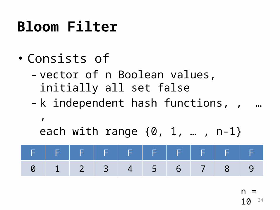
Bloom Filter
• Consists of – vector of n Boolean values, initially all set false– k independent hash functions, , … ,
each with range {0, 1, … , n-1}
F F F F F F F F F F
0 1 2 3 4 5 6 7 8 9
n = 10
35
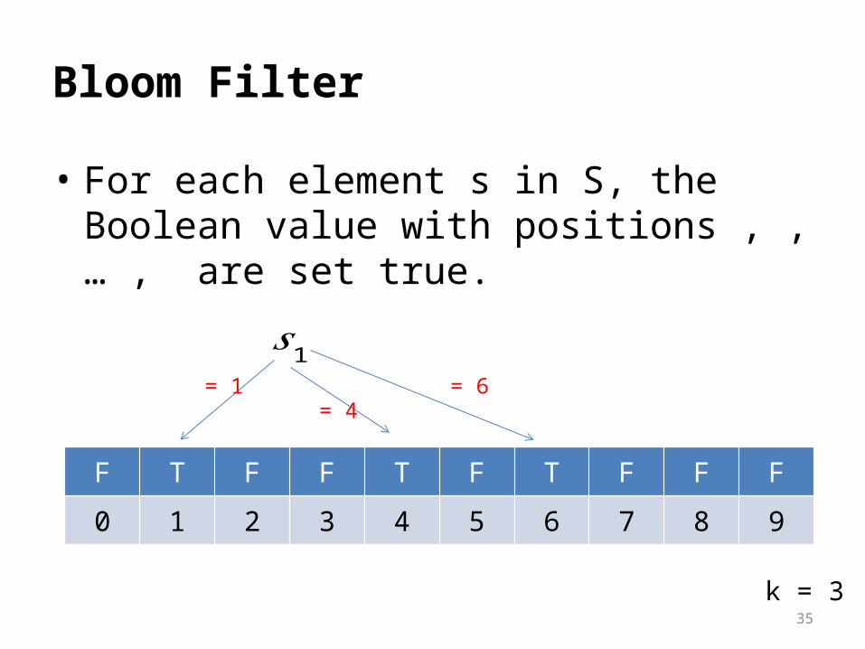
Bloom Filter
• For each element s in S, the Boolean value with positions , , … , are set true.
F T F F T F T F F F
0 1 2 3 4 5 6 7 8 9
𝑠1 = 1
= 4 = 6
k = 3
36
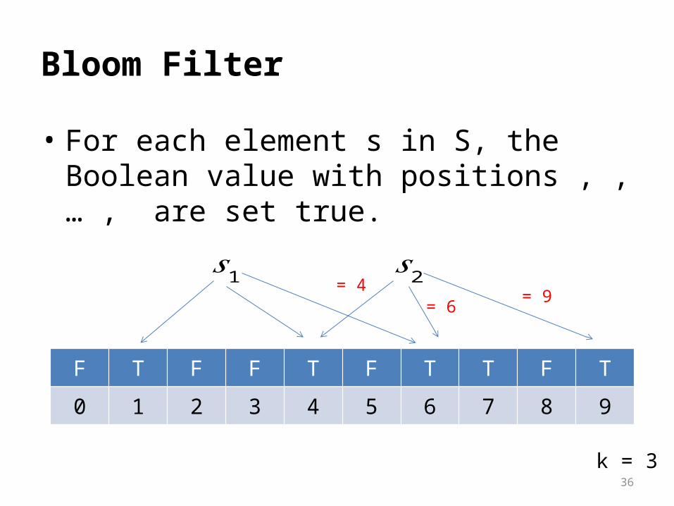
Bloom Filter
• For each element s in S, the Boolean value with positions , , … , are set true.
F T F F T F T T F T
0 1 2 3 4 5 6 7 8 9
𝑠1 𝑠2 = 4 = 6
= 9
k = 3

37
Error Types
• False Negative– Never happens for Bloom Filter
• False Positive– Answering “is there” on an element that is not in
the set
38
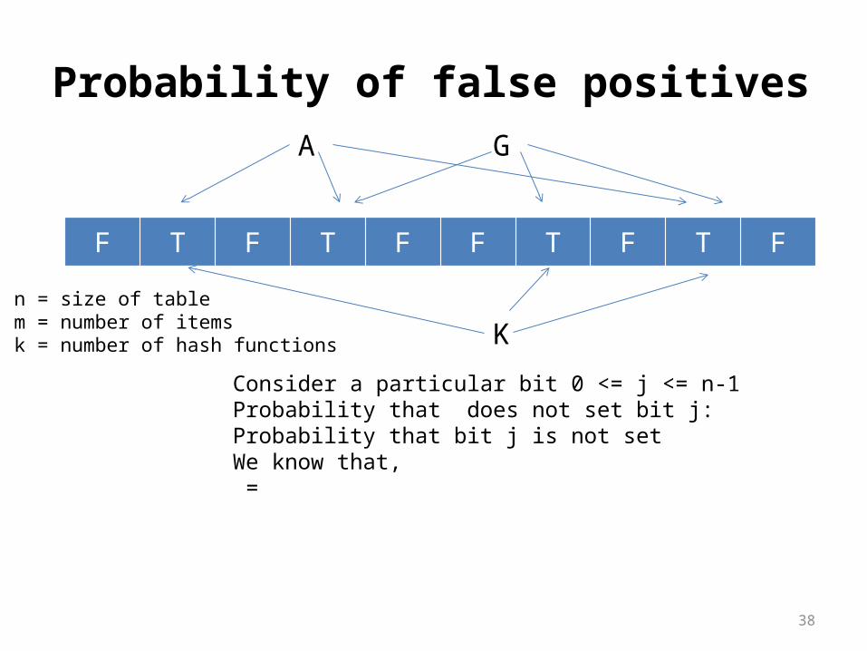
Probability of false positives
F T F T F F T F T F
A G
Kn = size of tablem = number of itemsk = number of hash functions
Consider a particular bit 0 <= j <= n-1Probability that does not set bit j: Probability that bit j is not set We know that, =

39
Probability of false positives
F T F T F F T F T F
A G
Kn = size of tablem = number of itemsk = number of hash functions
Probability of false positive = Note: All k bits of new element are already set
False positive probability can be minimized by choosing k = Upper Bound Probability would be
40
Bloom Filters: cons
• Small false positive probability• No deletions• Can not store associated objects
41
References
• Graham Cormode, Sketch Techniques for Approximate Query Processing, ATT Research
• Michael Mitzenmacher, Compressed Bloom Filters, Harvard University, Cambridge
42
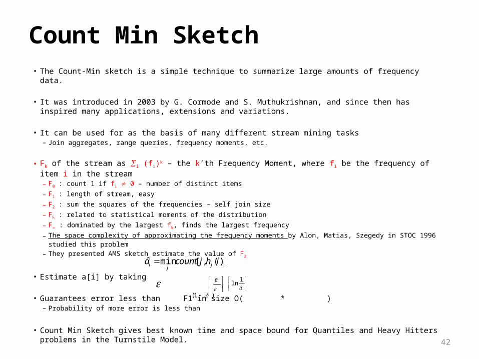
Count Min Sketch• The Count-Min sketch is a simple technique to summarize large amounts of frequency data.
• It was introduced in 2003 by G. Cormode and S. Muthukrishnan, and since then has inspired many applications, extensions and variations.
• It can be used for as the basis of many different stream mining tasks– Join aggregates, range queries, frequency moments, etc.
• Fk of the stream as i (fi)k – the k’th Frequency Moment, where fi be the frequency of item i in the stream– F0 : count 1 if fi 0 – number of distinct items
– F1 : length of stream, easy
– F2 : sum the squares of the frequencies – self join size
– Fk : related to statistical moments of the distribution
– F : dominated by the largest fk, finds the largest frequency– The space complexity of approximating the frequency moments by Alon, Matias, Szegedy in STOC 1996 studied this
problem– They presented AMS sketch estimate the value of F2
• Estimate a[i] by taking
• Guarantees error less than F1 in size O( * ) – Probability of more error is less than
• Count Min Sketch gives best known time and space bound for Quantiles and Heavy Hitters problems in the Turnstile Model.
1
ln
e
)](,[minˆ ihjcounta jj
i
)1(

43
Count Min Sketch– Model input data stream as vector
Where initially – The update is
))(),(,),(()( 1 tatatata ni
iai 0)0(
),( tt ci)1()( tata ii tii
tii ctatatt
)1()(
• A Count-Min (CM) Sketch with parameters is represented by a two-dimensional array (a small summary of input) counts with width and depth .
Given parameters , set and . Each entry of the array is initially zero.
hash functions are chosen uniformly at random from a pairwise independent family which map vector entry to [1…w]. i.e.
),( w ],[]1,1[: wdcountcountd
),(
e
w
1
lnd
d}1{}1{:,,1 wnhh d
Update procedure :

44
Count Min Sketch Algorithm

45
Example
46
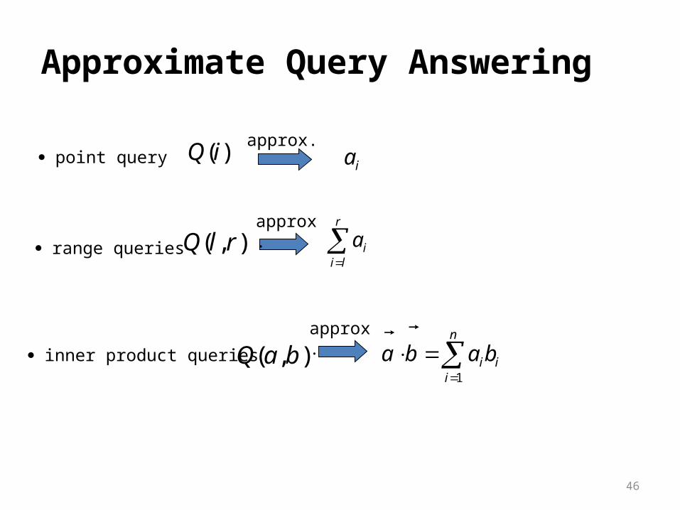
point queryapprox.
ia)(iQ
range queries ),( rlQapprox.
r
liia
inner product queries ),( baQ approx.
n
iiibaba
1
Approximate Query Answering

47
)(iQ )](,[minˆ ihjcounta jj
i
Non-negative case ( )
Theorem 1 ii aa ˆ ]ˆ[1
aaaP ii
0)( tati
Point Query
PROOF : Introduce indicator variables
kjiI ,, ))()(()( khihki jj 1 if
0 otherwise
ewkhihIE jjkji
1)]()(Pr[)( ,,
Define the variable
n
kkkjiji aIX
1,,,
By construction, jiij Xaihjcount ,)](,[ ij aihjcount )](,[min

48
For the other direction, observe that
])](,[.Pr[]ˆPr[11
aaihjcountjaaa ijii
].Pr[1, aaXaj ijii
djiji eXeEXj )](.Pr[ ,,
Markov inequality
0)(
]Pr[ tt
XEtX
■
n
kkjik
n
kkkjiji a
eIEaaIEXE
11,,
1,,, )()(
Analysis
49
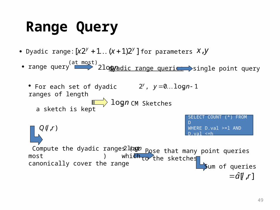
Dyadic range: ]2)1(12[ yy xx for parameters yx,
range query dyadic range queriesn2log2 single point query(at most)
· For each set of dyadic ranges of length a sketch is kept n2log CM Sketches
1log0,2 2 nyy
Range Query
Pose that many point queries to the sketches
),( rlQ
Compute the dyadic ranges (at most ) which canonically cover the range
Sum of queries
],[ˆ rla
n2log2
SELECT COUNT (*) FROM DWHERE D.val >=l AND D.val <=h
50
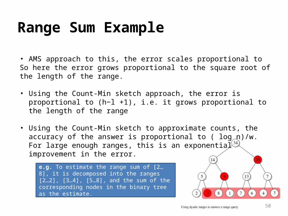
Range Sum Example
• AMS approach to this, the error scales proportional to So here the error grows proportional to the square root of the length of the range.
• Using the Count-Min sketch approach, the error is proportional to (h−l +1), i.e. it grows proportional to the length of the range
• Using the Count-Min sketch to approximate counts, the accuracy of the answer is proportional to ( log n)/w. For large enough ranges, this is an exponential improvement in the error.
e.g. To estimate the range sum of [2…8], it is decomposed into the ranges [2…2], [3…4], [5…8], and the sum of the corresponding nodes in the binary tree as the estimate.
51
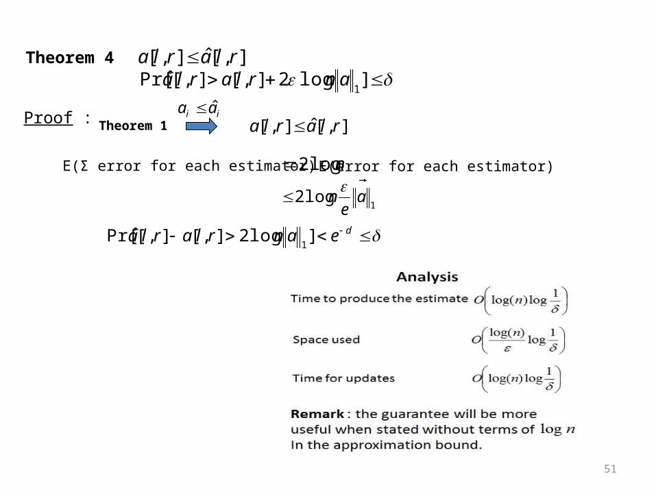
Theorem 4 ],[ˆ],[ rlarla ]log2],[],[ˆPr[
1anrlarla
Proof : Theorem 1ii aa ˆ
],[ˆ],[ rlarla
E(Σ error for each estimator) nlog2 E(error for each estimator)
■
1log2 a
en
deanrlarla ]log2],[],[ˆPr[1

52
Set
w
kbaj kjcountkjcountba
1
],[],[)(
),( baQ
jjbaba
)(min)(
Inner Product Query
Theorem 3
)()( baba
])(Pr[11
bababa
Analysis Time to produce the estimate
Space used
Time for updates
)1
log1
(
O
)1
log1
(
O
)1
(log
O
The application of inner-product computation to Join size estimationApplication
Corollary The Join size of two relations on a particular attribute can be approximated up to with probability by keeping space
11ba 1
1
log1
O

53
ResourcesApplications
– Compressed Sensing– Networking– Databases– Eclectics (NLP, Security, Machine Learning, ...)
Details– Extensions of the Count-Min Sketch– Implementations and code
List of open problems in streaming– Open problems in streaming
54
References for Count Min Sketch• Basics
– G. Cormode and S. Muthukrishnan. An improved data stream summary: The count-min sketch and its applications. LATIN 2004, J. Algorithm 58-75 (2005) .– G. Cormode and S. Muthukrishnan. Summarizing and mining skewed data streams. SDM 2005. – G. Cormode and S. Muthukrishnan. Approximating data with the count-min data structure. IEEE Software, (2012).
• Journal– Alon, Noga; Matias, Yossi; Szegedy, Mario (1999), "The space complexity of approximating the frequency moments", Journal of Computer and System Sciences
58 (1): 137–147.
• Surveys– Network Applications of Bloom Filters: A Survey. Andrei Broder and Michael Mitzenmacher. Internet Mathematics Volume 1, Number 4 (2003), 485-509.– Article from "Encyclopedia of Database Systems" on Count-Min Sketch Graham Cormode 09. 5 page summary of the sketch and its applications.– A survey of synopsis construction in data streams. Charu Aggarwal.
• Coverage in Textbooks– Probability and Computing: Randomized Algorithms and Probabilistic Analysis. Michael Mitzenmacher, Eli Upfal. Cambridge University Press, 2005. Describes
Count-Min sketch over pages 329--332– Internet Measurement: Infrastructure, Traffic and Applications. Mark Crovella, Bala Krishnamurthy. Wiley 2006.
• Tutorials– Advanced statistical approaches for network anomaly detection. Christian Callegari. ICIMP 10 Tutorial.– Video explaining sketch data structures with emphasis on CM sketch Graham Cormode.
• Lectures– Data Stream Algorithms. Notes from a series of lectures by S. Muthu Muthukrishnan. – Data Stream Algorithms. Lecture notes, Chapter 3. Amit Chakrabarti. Fall 09. – Probabilistic inequalities and CM sketch. John Byers. Fall 2007.
Overview
• Introduction to Streaming Algorithms • Sampling Techniques • Sketching Techniques
Break• Counting Distinct Numbers• Q&A

Overview
• Introduction to Streaming Algorithms • Sampling Techniques • Sketching Techniques
Break• Counting Distinct Numbers• Q&A

57
Stream Model of Computation
10
11
1
0
1
0
0
1
1
Increasi
ng time
Main Memory (Synopsis Data Structures)
Data Stream
Memory: poly(1/ε, log N)
Query/Update Time: poly(1/ε, log N)
N: # items so far, or window size
ε: error parameter

58
Counting Distinct Elements -Motivation
• Motivation: Various applications
40 Gbps
8MB SRAM
• Port Scanning• DDoS Attacks• Traffic
Accounting• Traffic
Engineering• Quality of
Service
IP1 IP2 IP1 IP3 IP1 IP2
Packet Filtering: No of Packets – 6 (n) No of Distinct Packets – 3 (m)

59
Counting Distinct Elements - Problem
• Problem: Given a stream of values. Let be the number of distinct elements in . Find under the constraints for algorithms on data streams.
• Constraints: – Elements in stream are presented sequentially and single pass is
allowed.– Limited space to operate. Expected space complexity or smaller.– Estimation Guarantees : With Error and high proability

60
Naïve Approach
• Counter C(i) for each domain value i in [n]• Initialize counters C(i) 0• Scan X incrementing appropriate counters• Solution: Distinct Values = Number of C(i) > 0• Problem
– Memory size M << n– Space O(n) – possibly n >> m
(e.g., when counting distinct words in web crawl)– Time O(n)

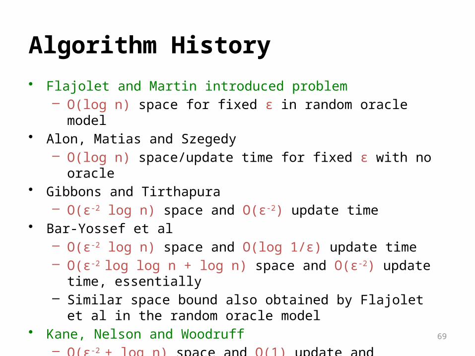
Algorithm History• Flajolet and Martin introduced problem
– O(log n) space for fixed ε in random oracle model• Alon, Matias and Szegedy
– O(log n) space/update time for fixed ε with no oracle• Gibbons and Tirthapura
– O(ε-2 log n) space and O(ε-2) update time• Bar-Yossef et al
– O(ε-2 log n) space and O(log 1/ε) update time– O(ε-2 log log n + log n) space and O(ε-2) update time, essentially– Similar space bound also obtained by Flajolet et al in the random
oracle model• Kane, Nelson and Woodruff
– O(ε-2 + log n) space and O(1) update and reporting time– All time complexities are in unit-cost RAM model
61

62
Flajolet-Martin Approach
• Hash function h: map n elements tobits (uniformly distributed over the set of binary strings of length L)
• For y any non-negative integer, define bit(y, k) = kth bit in the binary representation of y
if y >0
if y = 0
represents the position of the least significant –bit in the binary representation of y
63
Flajolet-Martin Approach
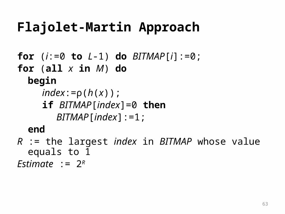
for (i:=0 to L-1) do BITMAP[i]:=0;for (all x in M) do
beginindex:=ρ(h(x));if BITMAP[index]=0 then
BITMAP[index]:=1;end
R := the largest index in BITMAP whose value equals to 1Estimate := 2R

64
Examples of bit(y, k) & ρ(y)
• y=10=(1010)2
– bit(y,0)=0 bit(y,1)=1 bit(y,2)=0 bit(y,3)=1
–
int y binary format
ρ(y)
0 0000 4 (=L)
1 0001 0
2 0010 1
3 0011 0
4 0100 2
5 0101 0
6 0110 1
7 0111 0
8 1000 3
k
k
kybity 2),(0

65
Flajolet-Martin Approach – Estimate Example
• Part of a Unix manual file M of size 26692 lines is loaded of which 16405 are distinct.
• If the final BITMAP looks like this:0000,0000,1100,1111,1111,1111
• The left most 1 appears at position 15• We say there are around 215 distinct elements in the
stream. But 214 = 16384.• Estimate where is the correction factor.

66
Flajolet-Martin* Approach
• Pick a hash function h that maps each of the n elements to at least log2n bits.
• For each stream element a, let r (a ) be the number of trailing 0’s in h (a ).
• Record R = the maximum r (a ) seen.• Estimate = 2R.
* Really based on a variant due to AMS (Alon, Matias, and Szegedy)

67
Why It Works
• The probability that a given h (a ) ends in at least r 0’s is 2-r.
• If there are m different elements, the probability that R ≥ r is 1 – (1 - 2-r )m.
Probability anygiven h(a) ends infewer than r 0’s.
Prob. all h(a)’send in fewer thanr 0’s.
68
Why It Works (2)
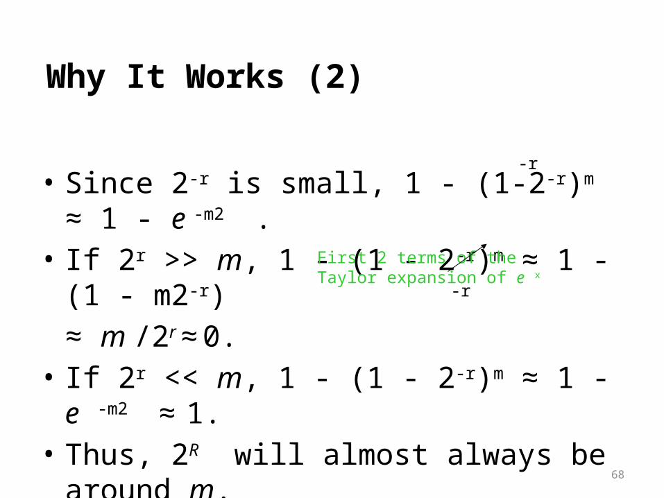
• Since 2-r is small, 1 - (1-2-r)m ≈ 1 - e -m2 .• If 2r >> m, 1 - (1 - 2-r)m ≈ 1 - (1 - m2-r) ≈ m /2r ≈ 0.• If 2r << m, 1 - (1 - 2-r)m ≈ 1 - e -m2 ≈ 1.• Thus, 2R will almost always be around m.
-r
-r
First 2 terms of theTaylor expansion of e x
Algorithm History• Flajolet and Martin introduced problem
– O(log n) space for fixed ε in random oracle model• Alon, Matias and Szegedy
– O(log n) space/update time for fixed ε with no oracle• Gibbons and Tirthapura
– O(ε-2 log n) space and O(ε-2) update time• Bar-Yossef et al
– O(ε-2 log n) space and O(log 1/ε) update time– O(ε-2 log log n + log n) space and O(ε-2) update time, essentially– Similar space bound also obtained by Flajolet et al in the random
oracle model• Kane, Nelson and Woodruff
– O(ε-2 + log n) space and O(1) update and reporting time– All time complexities are in unit-cost RAM model
69

70
An Optimal Algorithm for the Distinct Elements Problem
Daniel M. Kane, Jelani Nelson, David P. Woodruff

71
Overview
• Computes a approximation using an optimal Θ(ε-2 + log n) bits of space with 2/3 success probability, where 0 < ε < 1 is given
• Process each stream update in Θ(1) worst-case time

72
Foundation technique 1
• If it is known that R=Θ(F0) then estimation becomes easier
• Run a constant-factor estimation at the end of the stream to achieve R before the main estimation algorithm ROUGH ESTIMATOR
73
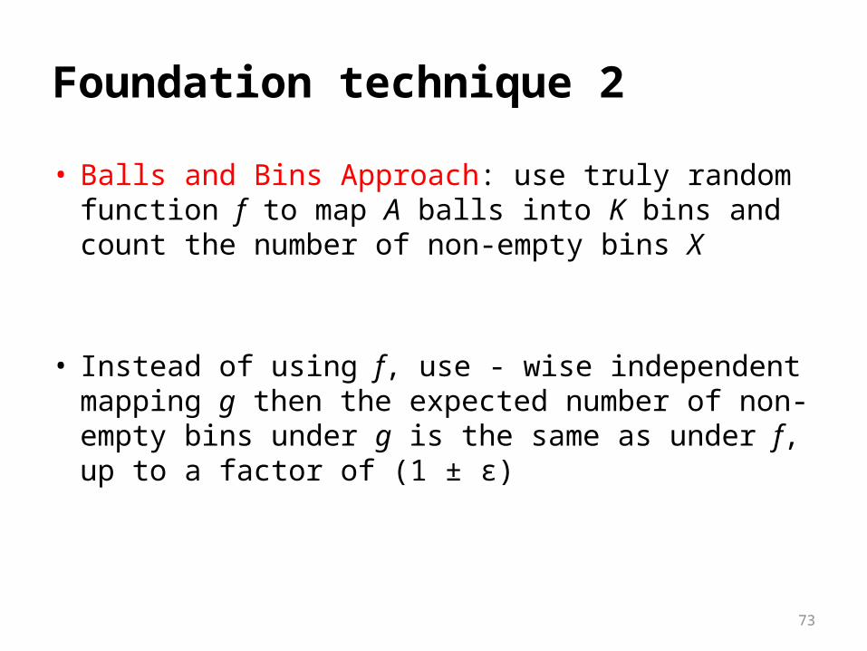
Foundation technique 2
• Balls and Bins Approach: use truly random function f to map A balls into K bins and count the number of non-empty bins X
• Instead of using f, use - wise independent mapping g then the expected number of non-empty bins under g is the same as under f, up to a factor of (1 ± ε)
74
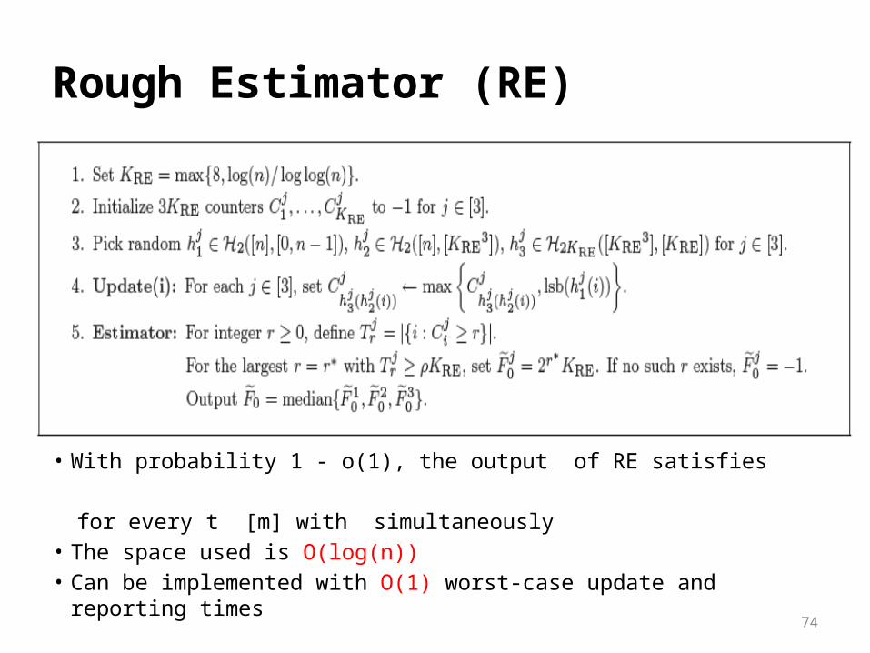
Rough Estimator (RE)
• With probability 1 - o(1), the output of RE satisfies for every t [m] with simultaneously
• The space used is O(log(n))• Can be implemented with O(1) worst-case update and reporting times

75
Main Algorithm(1)
• The algorithm outputs a value which is with probability at least 11/20 as long as
76
Main Algorithm (2)
• A: keeps track of the amount of storage required to store all the
• est: is such that is a -approximation to , and is obtained via Rough Estimator
• b: is such that we expect to be at all points t in the stream.

77
Main Algorithm (3)
• Subsample the stream at geometrically decreasing rates • Perform balls and bins at each level• When i appears in stream, put a ball in cell [g(i), h(i)]• For each column, store the largest row containing a ball• Estimate based on these numbers

78
Prove Space Complexity
• The hash functions h1, h2 each require bits to store• The hash function h3 takes = O()) bits to store• The value b takes bits• The value A never exceeds the total number of bits to store
all counters, which is , and thus A can be represented in bits
• The counters never in total consume more than bits by construction, since we output FAIL if they ever would
• The Rough Estimator and est use O(log(n)) bits
Total space complexity:
79
Prove Time Complexity
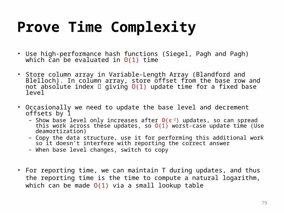
• Use high-performance hash functions (Siegel, Pagh and Pagh) which can be evaluated in O(1) time
• Store column array in Variable-Length Array (Blandford and Blelloch). In column array, store offset from the base row and not absolute index giving O(1) update time for a fixed base level
• Occasionally we need to update the base level and decrement offsets by 1– Show base level only increases after Θ(ε-2) updates, so can spread this work
across these updates, so O(1) worst-case update time (Use deamortization)– Copy the data structure, use it for performing this additional work so it doesn’t
interfere with reporting the correct answer– When base level changes, switch to copy
• For reporting time, we can maintain T during updates, and thus the reporting time is the time to compute a natural logarithm, which can be made O(1) via a small lookup table

80
References
• Blandford, Blelloch. Compact dictionaries for variable-length keys and data with applications. ACM Transactions on Algorithms. 2008.
• D. M. Kane, J. Nelson, and D. P. Woodruff. An optimal algorithm for the distinct elements problem. In Proc. 29th ACM Symposium on Principles of Database Systems, pages 41-52. 2010.
• Pagh, Pagh. Uniform Hashing in Constant Time and Optimal Space. SICOMP 2008.
• Siegel. On Universal Classes of Uniformly Random Constant-Time Hash Functions. SICOMP 2004.
81
Summary• We introduced Streaming Algorithms• Sampling Algorithms
– Reservoir Sampling – Priority Sampling
• Sketch Algorithms– Bloom Filter– Count-Min Sketch
• Counting Distinct Elements– Flajolet-Martin Algorithm– Optimal Algorithm
82
Q & A