Embed Size (px)
DESCRIPTION
System Software Ebook
Citation preview

ANNA UNIVERSITY TIRUNELVELI / REGULATION 2008 CS54 – SYSTEM SOFTWARE
©EINSTEIN COLLEGE OF ENGINEERING Page 1 of 131
AIM
To have an understanding of foundations of design of assemblers, loaders, linkers, and macro processors.
OBJECTIVES
To understand the relationship between system software and machine architecture.
To know the design and implementation of assemblers
To know the design and implementation of linkers and loaders.
To have an understanding of macroprocessors.
To have an understanding of system software tools.
UNIT I INTRODUCTION 8
System software and machine architecture – The Simplified Instructional Computer (SIC) - Machine architecture - Data and instruction formats - addressing modes - instruction sets - I/O and programming. UNIT II ASSEMBLERS 10 Basic assembler functions - A simple SIC assembler – Assembler algorithm and data structures - Machine dependent assembler features - Instruction formats and addressing
modes – Program relocation - Machine independent assembler features - Literals – Symbol-defining statements – Expressions - One pass assemblers and Multi pass assemblers - Implementation example - MASM assembler. UNIT III LOADERS AND LINKERS 9 Basic loader functions - Design of an Absolute Loader – A Simple Bootstrap Loader - Machine dependent loader features - Relocation – Program Linking – Algorithm and Data Structures for Linking Loader - Machine-independent loader features - Automatic
Library Search – Loader Options - Loader design options - Linkage Editors – Dynamic Linking – Bootstrap Loaders - Implementation example - MSDOS linker. UNIT IV MACRO PROCESSORS 9
Basic macro processor functions - Macro Definition and Expansion – Macro Processor Algorithm and data structures - Machine-independent macro processor features - Concatenation of Macro Parameters – Generation of Unique Labels – Conditional Macro Expansion – Keyword Macro Parameters-Macro within Macro-Implementation example - MASM Macro Processor – ANSI C Macro language. UNIT V SYSTEM SOFTWARE TOOLS 9 Text editors - Overview of the Editing Process - User Interface – Editor Structure. - Interactive debugging systems - Debugging functions and capabilities – Relationship
with other parts of the system – User-Interface Criteria.
TEXT BOOK 1. Leland L. Beck, “System Software – An Introduction to Systems Programming”, 3rd Edition, Pearson Education Asia, 2006. REFERENCES
1. D. M. Dhamdhere, “Systems Programming and Operating Systems”, Second Revised Edition, Tata McGraw-Hill, 2000.
2. John J. Donovan “Systems Programming”, Tata McGraw-Hill Edition, 2000.

ANNA UNIVERSITY TIRUNELVELI / REGULATION 2008 CS54 – SYSTEM SOFTWARE
©EINSTEIN COLLEGE OF ENGINEERING Page 2 of 131
UNIT I - INTRODUCTION The subject introduces the design and implementation of system software. Software is set of instructions or programs written to carry out certain task on digital computers. It is classified into system software and application software.
System software consists of a variety of programs that support the operation of a computer. This software makes it possible for the user to focus on an application or other problem to be solved, without needing to know the details of how the machine works internally Eg. Operating system, compiler, assembler, macro processor, loader or linker, debugger, text editor, database management systems (some of them) and, software engineering tools. Application software focuses on an application or problem to be solved. System software consists of a variety of programs that support the operation of a computer. DIFFERENT STEPS INVOLVED IN USING A HIGH LEVEL LANGUAGE
Types of system s/w that has been used by us in a C program Step 1: A program written (create & modify) in High level language ( C, C++, pascal
typed in text editor Step 2: Translated into machine language (object program) using compiler. The compiler
in turn store the .obj into the secondary device Step 3. The resulting machine language program was loaded into memory & prepared
for execution by a loader or liker. There are diff loading schemes viz. absolute, relocating and direct linking. In general the loader must load relocate and link the object program
Step 4: debugger -> helps t detect errors in the program DIFFERENT STEPS INVOLVED IN USING ASSEMBLY LANGUAGE Step 1: Program written using macro instructions to read & write data Step 2: Uses assembler, which probably included a macro processor to translate these
programs into machine language Step 3: loader or linker (prepared for execution) Step 4: tested using debugger All these processes are controlled by interacting withthe OS of the computer UNIX or DOS –> Keyboard Commands MacOs or Windows -> Menus -> Click
SYSTEM SOFTWARE AND MACHINE ARCHITECTURE
One characteristic in which most system software differs from application software is machine dependency. System software – support operation and use of computer.
Application software - solution to a problem. Assembler translates mnemonic instructions into machine code. The instruction formats, addressing modes etc., are of direct concern in assembler design. Similarly, Compilers must generate machine language code, taking into account such hardware characteristics as the

ANNA UNIVERSITY TIRUNELVELI / REGULATION 2008 CS54 – SYSTEM SOFTWARE
©EINSTEIN COLLEGE OF ENGINEERING Page 3 of 131
number and type of registers and the machine instructions available. Operating systems are
directly concerned with the management of nearly all of the resources of a computing system. There are aspects of system software that do not directly depend upon the type of computing system, general design and logic of an assembler, general design and logic of a compiler and, code optimization techniques, which are independent of target machines. Likewise, the process of linking together independently assembled subprograms does not usually depend on the computer being used. THE SIMPLIFIED INSTRUCTIONAL COMPUTER (SIC)
Simplified Instructional Computer (SIC) is a hypothetical computer that includes the hardware features most often found on real machines. There are two versions of SIC, they are, standard model (SIC), and, extension version (SIC/XE) (extra equipment or extra expensive). SIC MACHINE ARCHITECTURE We discuss here the SIC machine architecture with respect to its Memory and Registers, Data Formats, Instruction Formats, Addressing Modes, Instruction Set, Input and Output Memory
There are 215 bytes in the computer memory, that is 32,768 bytes , It uses Little Endian format to store the numbers, 3 consecutive bytes form a word , each location in memory contains 8-bit bytes. Registers
There are five registers, each 24 bits in length. Their mnemonic, number and use are given in the following table.
Mnemonic Number Use
A 0 Accumulator; used for arithmetic operations
X 1 Index register; used for addressing
L 2 Linkage register; JSUB
PC 8 Program counter
SW 9 Status word, including CC

ANNA UNIVERSITY TIRUNELVELI / REGULATION 2008 CS54 – SYSTEM SOFTWARE
©EINSTEIN COLLEGE OF ENGINEERING Page 4 of 131
Data Formats
Integers are stored as 24-bit binary numbers , 2‟s complement representation is used for negative values, characters are stored using their 8-bit ASCII codes, No floating-point hardware on the standard version of SIC. Instruction Formats
Opcode(8) x Address (15)
All machine instructions on the standard version of SIC have the 24-bit format as shown above Addressing Modes
Mode Indication Target address calculation
Direct x = 0 TA = address
Indexed x = 1 TA = address + (x)
There are two addressing modes available, which are as shown in the above table. Parentheses are used to indicate the contents of a register or a memory location. Instruction Set
SIC provides, load and store instructions (LDA, LDX, STA, STX, etc.). Integer arithmetic operations: (ADD, SUB, MUL, DIV, etc.). All arithmetic operations involve register A and a word in memory, with the result being left in the register. Two instructions are provided for subroutine linkage. COMP compares the value in register A with a word in memory, this instruction sets a condition code CC to indicate the result. There are conditional jump instructions: (JLT, JEQ, JGT), these instructions test the setting of CC and jump accordingly. JSUB jumps to the subroutine placing the return address in register L, RSUB returns by jumping to the address contained in register L. Input and Output Input and Output are performed by transferring 1 byte at a time to or from the rightmost 8 bits of register A (accumulator). The Test Device (TD) instruction tests whether the addressed device is ready to send or receive a byte of data. Read Data (RD), Write Data (WD) are used for reading or writing the data. Data movement and Storage Definition LDA, STA, LDL, STL, LDX, STX ( A- Accumulator, L – Linkage Register, X – Index Register), all uses 3-byte word. LDCH, STCH associated with characters uses 1-byte. There are no memory-memory move instructions.

ANNA UNIVERSITY TIRUNELVELI / REGULATION 2008 CS54 – SYSTEM SOFTWARE
©EINSTEIN COLLEGE OF ENGINEERING Page 5 of 131
Storage definitions are WORD - ONE-WORD CONSTANT RESW - ONE-WORD VARIABLE BYTE - ONE-BYTE CONSTANT RESB - ONE-BYTE VARIABLE Example Programs (SIC) Example 1(Simple data and character movement operation)
LDA FIVE STA ALPHA LDCH CHARZ STCH C1 . ALPHA RESW 1 FIVE WORD 5 CHARZ BYTE C‟Z‟ C1 RESB 1 Example 2( Arithmetic operations) LDA ALPHA ADD INCR SUB ONE STA BEETA …….. …….. …….. …….. ONE WORD 1 ALPHA RESW 1 BEETA RESW 1 INCR RESW 1 Example 3(Looping and Indexing operation)
LDX ZERO : X = 0 MOVECH LDCH STR1, X : LOAD A FROM STR1 STCH STR2, X : STORE A TO STR2 TIX ELEVEN : ADD 1 TO X, TEST JLT MOVECH . . . STR1 BYTE C „HELLO WORLD‟ STR2 RESB 11 ZERO WORD 0 ELEVEN WORD 11

ANNA UNIVERSITY TIRUNELVELI / REGULATION 2008 CS54 – SYSTEM SOFTWARE
©EINSTEIN COLLEGE OF ENGINEERING Page 6 of 131
Example 4( Input and Output operation)
INLOOP TD INDEV : TEST INPUT DEVICE JEQ INLOOP : LOOP UNTIL DEVICE IS READY RD INDEV : READ ONE BYTE INTO A STCH DATA : STORE A TO DATA . . OUTLP TD OUTDEV : TEST OUTPUT DEVICE JEQ OUTLP : LOOP UNTIL DEVICE IS READY LDCH DATA : LOAD DATA INTO A WD OUTDEV : WRITE A TO OUTPUT DEVICE . . INDEV BYTE X „F5‟ : INPUT DEVICE NUMBER OUTDEV BYTE X „08‟ : OUTPUT DEVICE NUMBER DATA RESB 1 : ONE-BYTE VARIABLE Example 5 (To transfer two hundred bytes of data from input device to memory)
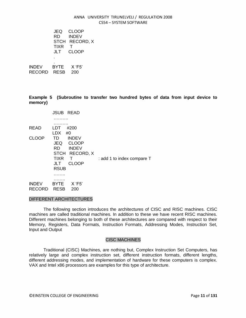
LDX ZERO CLOOP TD INDEV JEQ CLOOP RD INDEV STCH RECORD, X TIX B200 JLT CLOOP . . INDEV BYTE X „F5‟ RECORD RESB 200 ZERO WORD 0 B200 WORD 200 Example 6 (Subroutine to transfer two hundred bytes of data from input device to memory)
JSUB READ …………. …………. READ LDX ZERO CLOOP TD INDEV JEQ CLOOP RD INDEV STCH RECORD, X TIX B200 : add 1 to index compare 200 (B200)

ANNA UNIVERSITY TIRUNELVELI / REGULATION 2008 CS54 – SYSTEM SOFTWARE
©EINSTEIN COLLEGE OF ENGINEERING Page 7 of 131
JLT CLOOP RSUB …….. …….. INDEV BYTE X „F5‟ RECORD RESB 200 ZERO WORD 0 B200 WORD 200
SIC/XE MACHINE ARCHITECTURE
Memory
Maximum memory available on a SIC/XE system is 1 Megabyte (220 bytes) Registers
Additional B, S, T, and F registers are provided by SIC/XE, in addition to the registers of SIC
Mnemonic Number Special use
B 3 Base register
S 4 General working register
T 5 General working register
F 6 Floating-point accumulator (48 bits)
Floating-point data type
There is a 48-bit floating-point data type, F*2(e-1024)
1 11 36
s exponent fraction
Instruction Formats
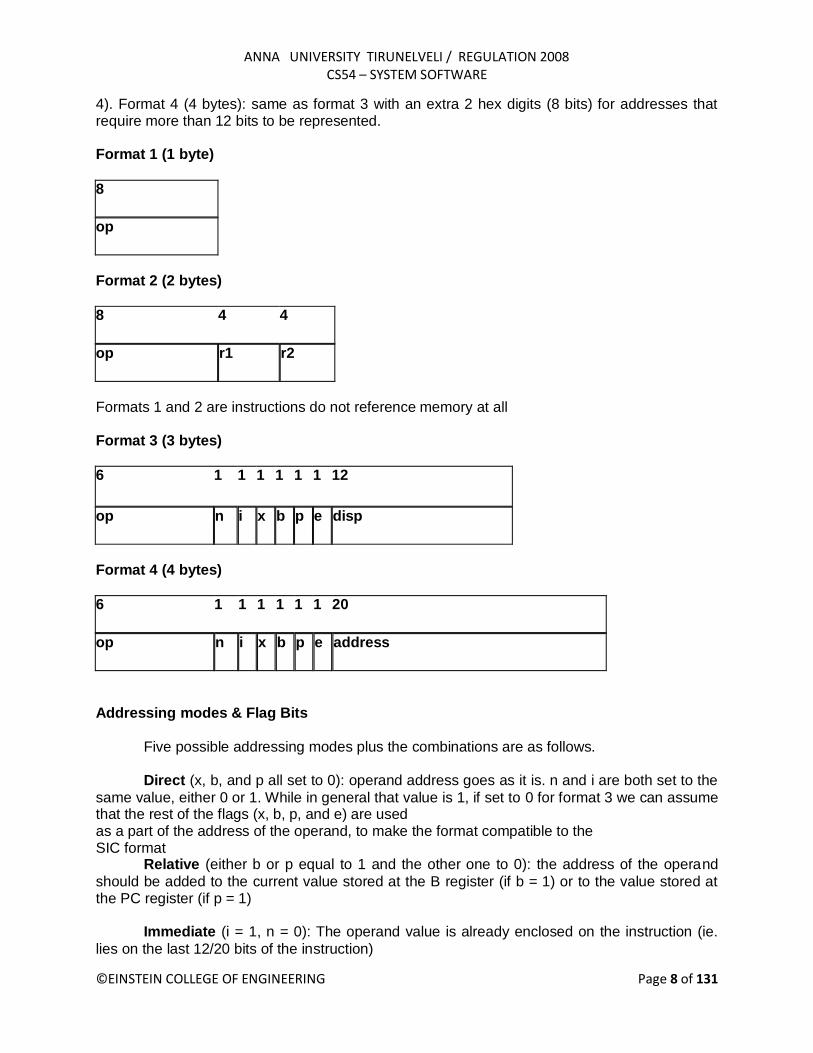
The new set of instruction formats for SIC/XE machine architecture are as follows. Format 1 (1 byte): contains only operation code (straight from table). Format 2 (2 bytes): first eight bits for operation code, next four for register 1 and following four for register 2. The numbers for the registers go according to the numbers indicated at the registers section (ie, register T is replaced by hex 5, F is replaced by hex 6). Format 3 (3 bytes): First 6 bits contain operation code, next 6 bits contain flags, last 12 bits contain displacement for the address of the operand. Operation code uses only 6 bits, thus the second hex digit will be affected by the values of the first two flags (n and i). The flags, in order, are: n, i, x, b, p, and e. Its functionality is explained in the next section. The last flag e indicates the instruction format (0 for 3 and 1 for
ANNA UNIVERSITY TIRUNELVELI / REGULATION 2008 CS54 – SYSTEM SOFTWARE
©EINSTEIN COLLEGE OF ENGINEERING Page 8 of 131
4). Format 4 (4 bytes): same as format 3 with an extra 2 hex digits (8 bits) for addresses that require more than 12 bits to be represented. Format 1 (1 byte)
8
op
Format 2 (2 bytes)
8 4 4
op r1 r2
Formats 1 and 2 are instructions do not reference memory at all Format 3 (3 bytes)
6 1 1 1 1 1 1 12
op n i x b p e disp
Format 4 (4 bytes)
6 1 1 1 1 1 1 20
op n i x b p e address
Addressing modes & Flag Bits
Five possible addressing modes plus the combinations are as follows. Direct (x, b, and p all set to 0): operand address goes as it is. n and i are both set to the
same value, either 0 or 1. While in general that value is 1, if set to 0 for format 3 we can assume that the rest of the flags (x, b, p, and e) are used as a part of the address of the operand, to make the format compatible to the SIC format Relative (either b or p equal to 1 and the other one to 0): the address of the operand
should be added to the current value stored at the B register (if b = 1) or to the value stored at the PC register (if p = 1) Immediate (i = 1, n = 0): The operand value is already enclosed on the instruction (ie.
lies on the last 12/20 bits of the instruction)

ANNA UNIVERSITY TIRUNELVELI / REGULATION 2008 CS54 – SYSTEM SOFTWARE
©EINSTEIN COLLEGE OF ENGINEERING Page 9 of 131
Indirect (i = 0, n = 1): The operand value points to an address that holds the address for the operand value. Indexed (x = 1): value to be added to the value stored at the register x to obtain real
address of the operand. This can be combined with any of the previous modes except immediate. The various flag bits used in the above formats have the following meanings e - e = 0 means format 3, e = 1 means format 4 Bits x,b,p: Used to calculate the target address using relative, direct, and indexed addressing Modes Bits i and n: Says, how to use the target address b and p - both set to 0, disp field from format 3 instruction is taken to be the target address. For a format 4 bits b and p are normally set to 0, 20 bit address is the target address x - x is set to 1, X register value is added for target address calculation i=1, n=0 Immediate addressing, TA: TA is used as the operand value, no memory reference i=0, n=1 Indirect addressing, ((TA)): The word at the TA is fetched. Value of TA is taken as the
address of the operand value i=0, n=0 or i=1, n=1 Simple addressing, (TA):TA is taken as the address of the operand value Two new relative addressing modes are available for use with instructions assembled using format 3.
Mode Indication Target address calculation
Base relative b=1,p=0 TA=(B)+ disp
(0disp 4095)
Program-counter relative
b=0,p=1 TA=(PC)+ disp
(-2048disp 2047)
Instruction Set SIC/XE provides all of the instructions that are available on the standard version. In addition we have, Instructions to load and store the new registers LDB, STB, etc, Floating-point arithmetic operations, ADDF, SUBF, MULF, DIVF, Register move instruction : RMO, Register-to-register arithmetic operations, ADDR, SUBR, MULR, DIVR and, Supervisor call instruction : SVC.

ANNA UNIVERSITY TIRUNELVELI / REGULATION 2008 CS54 – SYSTEM SOFTWARE
©EINSTEIN COLLEGE OF ENGINEERING Page 10 of 131
Input and Output
There are I/O channels that can be used to perform input and output while the CPU is executing other instructions. Allows overlap of computing and I/O, resulting in more efficient system operation. The instructions SIO, TIO, and HIO are used to start, test and halt the operation of I/O channels. Example Programs (SIC/XE) Example 1 (Simple data and character movement operation)
LDA #5 STA ALPHA LDA #90 STCH C1 . . ALPHA RESW 1 C1 RESB 1 Example 2(Arithmetic operations)
LDS INCR LDA ALPHA ADD S,A SUB #1 STA BEETA …………. ………….. ALPHA RESW 1 BEETA RESW 1 INCR RESW 1 Example 3(Looping and Indexing operation) LDT #11 LDX #0 : X = 0 MOVECH LDCH STR1, X : LOAD A FROM STR1 STCH STR2, X : STORE A TO STR2 TIXR T : ADD 1 TO X, TEST (T) JLT MOVECH ………. ………. ……… STR1 BYTE C „HELLO WORLD‟ STR2 RESB 11 Example 4 (To transfer two hundred bytes of data from input device to memory)
LDT #200 LDX #0 CLOOP TD INDEV
ANNA UNIVERSITY TIRUNELVELI / REGULATION 2008 CS54 – SYSTEM SOFTWARE
©EINSTEIN COLLEGE OF ENGINEERING Page 11 of 131
JEQ CLOOP RD INDEV STCH RECORD, X TIXR T JLT CLOOP . . INDEV BYTE X „F5‟ RECORD RESB 200 Example 5 (Subroutine to transfer two hundred bytes of data from input device to memory) JSUB READ ………. ………. READ LDT #200 LDX #0 CLOOP TD INDEV JEQ CLOOP RD INDEV STCH RECORD, X TIXR T : add 1 to index compare T JLT CLOOP RSUB …….. …….. INDEV BYTE X „F5‟ RECORD RESB 200 DIFFERENT ARCHITECTURES The following section introduces the architectures of CISC and RISC machines. CISC machines are called traditional machines. In addition to these we have recent RISC machines. Different machines belonging to both of these architectures are compared with respect to their Memory, Registers, Data Formats, Instruction Formats, Addressing Modes, Instruction Set, Input and Output
CISC MACHINES Traditional (CISC) Machines, are nothing but, Complex Instruction Set Computers, has relatively large and complex instruction set, different instruction formats, different lengths, different addressing modes, and implementation of hardware for these computers is complex. VAX and Intel x86 processors are examples for this type of architecture.

ANNA UNIVERSITY TIRUNELVELI / REGULATION 2008 CS54 – SYSTEM SOFTWARE
©EINSTEIN COLLEGE OF ENGINEERING Page 12 of 131
VAX ARCHITECTURE Memory - The VAX memory consists of 8-bit bytes. All addresses used are byte addresses.
Two consecutive bytes form a word, Four bytes form a longword, eight bytes form a quadword, sixteen bytes form a octaword. All VAX programs operate in a virtual address space of 232 bytes , One half is called system space, other half process space. Registers – There are 16 general purpose registers (GPRs) , 32 bits each, named as R0 to R15, PC (R15), SP (R14), Frame Pointer FP ( R13), Argument Pointer AP (R12) ,Others available for general use. There is a Process status longword (PSL) – for flags. Data Formats - Integers are stored as binary numbers in byte, word, longword, quadword,
octaword. 2‟s complement notation is used for storing negative numbers. Characters are stored as 8-bit ASCII codes. Four different floating-point data formats are also available. Instruction Formats - VAX architecture uses variable-length instruction formats – op code 1 or
2 bytes, maximum of 6 operand specifiers depending on type of instruction. Tabak – Advanced Microprocessors (2nd edition) McGraw-Hill, 1995, gives more information. Addressing Modes - VAX provides a large number of addressing modes. They are Register
mode, register deferred mode, autoincrement, autodecrement, base relative, program-counter relative, indexed, indirect, and immediate. Instruction Set – Instructions are symmetric with respect to data type - Uses prefix – type of
operation, suffix – type of operands, a modifier – number of operands. For example, ADDW2 - add, word length, 2 operands, MULL3 - multiply, longwords, 3 operands CVTCL - conversion from word to longword. VAX also provides instructions to load and store multiple registers. Input and Output - Uses I/O device controllers. Device control registers are mapped to
separate I/O space. Software routines and memory management routines are used for input/output operations. PENTIUM PRO ARCHITECTURE Introduced by Intel in 1995. Memory - consists of 8-bit bytes, all addresses used are byte addresses. Two consecutive bytes form a word, four bytes form a double word (dword). Viewed as collection of segments, and, address = segment number + offset. There are code, data, stack , extra segments. Registers – There are 32-bit, eight GPRs, namely EAX, EBX, ECX, EDX, ESI, EDI, EBP, ESP. EAX, EBX, ECX, EDX – are used for data manipulation, other four are used to hold addresses. EIP – 32-bit contains pointer to next instruction to be executed. FLAGS is an 32 - bit flag register. CS, SS, DS, ES, FS, GS are the six 16-bit segment registers. Data Formats - Integers are stored as 8, 16, or 32 bit binary numbers, 2‟s complement for
negative numbers, BCD is also used in the form of unpacked BCD, packed BCD. There are three floating point data formats, they are single, double, and extended-precision. Characters are stored as one per byte – ASCII codes.

ANNA UNIVERSITY TIRUNELVELI / REGULATION 2008 CS54 – SYSTEM SOFTWARE
©EINSTEIN COLLEGE OF ENGINEERING Page 13 of 131
Instruction Formats – Instructions uses prefixes to specify repetition count, segment register,
following prefix (if present), an opcode ( 1 or 2 bytes), then number of bytes to specify operands, addressing modes. Instruction formats varies in length from 1 byte to 10 bytes or more. Opcode is always present in every instruction Addressing Modes - A large number of addressing modes are available. They are immediate mode, register mode, direct mode, and relative mode. Use of base register, index register with displacement is also possible. Instruction Set – This architecture has a large and complex instruction set, approximately 400
different machine instructions. Each instruction may have one, two or three operands. For example Register-to-register, register-to-memory, memory-to-memory, string manipulation, etc…are the some the instructions. Input and Output - Input is from an I/O port into register EAX. Output is from EAX to an I/O port
RISC MACHINES
RISC means Reduced Instruction Set Computers. These machines are intended to simplify the design of processors. They have Greater reliability, faster execution and less expensive processors. And also they have standard and fixed instruction length. Number of machine instructions, instruction formats, and addressing modes are relatively small. UltraSPARC Architecture and Cray T3E Architecture are examples of RISC machines. ULTRASPARC ARCHITECTURE Introduced by Sun Microsystems. SPARC – Scalable Processor ARChitecture. SPARC, SuperSPARC, UltraSPARC are upward compatible machines and share the same basic structure. Memory - Consists of 8-bit bytes, all addresses used are byte addresses. Two consecutive
bytes form a halfword, four bytes form a word , eight bytes form a double word. Uses virtual address space of 264 bytes, divided into pages. Registers - More than 100 GPRs, with 64 bits length each called Register file. There are 64
double precision floating-point registers, in a special floating-point unit (FPU). In addition to these, it contains PC, condition code registers, and control registers. Data Formats - Integers are stored as 8, 16, 32 or 64 bit binary numbers. Signed, unsigned for integers and 2‟s complement for negative numbers. Supports both big-endian and little-endian byte orderings. Floating-point data formats – single, double and quad-precision are available. Characters are stored as 8-bit ASCII value. Instruction Formats - 32-bits long, three basic instruction formats, first two bits identify the
format. Format 1 used for call instruction. Format 2 used for branch instructions. Format 3 used for load, store and for arithmetic operations. Addressing Modes - This architecture supports immediate mode, register-direct mode,PC-
relative, Register indirect with displacement, and Register indirect indexed.

ANNA UNIVERSITY TIRUNELVELI / REGULATION 2008 CS54 – SYSTEM SOFTWARE
©EINSTEIN COLLEGE OF ENGINEERING Page 14 of 131
Instruction Set – It has fewer than 100 machine instructions. The only instructions that access
memory are loads and stores. All other instructions are register-to-register operations. Instruction execution is pipelined – this results in faster execution, and hence speed increases. Input and Output - Communication through I/O devices is accomplished through memory. A
range of memory locations is logically replaced by device registers. When a load or store instruction refers to this device register area of memory, the corresponding device is activated. There are no special I/O instructions. CRAY T3E ARCHITECTURE Announced by Cray Research Inc., at the end of 1995 and is a massively parallel processing (MPP) system, contains a large number of processing elements (PEs), arranged in a three-dimensional network. Each PE consists of a DEC Alpha EV5 RISC processor, and local memory. Memory - Each PE in T3E has its own local memory with a capacity of from 64 megabytes to 2
gigabytes, consists of 8-bit bytes, all addresses used are byte addresses. Two consecutive bytes form a word, four bytes form a longword, eight bytes form a quadword. Registers – There are 32 general purpose registers(GPRs), with 64 bits length each called R0
through R31, contains value zero always. In addition to these, it has 32 floating-point registers, 64 bits long, and 64-bit PC, status , and control registers. Data Formats - Integers are stored as long and quad word binary numbers. 2‟s complement
notation for negative numbers. Supports only little-endian byte orderings. Two different floating-point data formats – VAX and IEEE standard. Characters stored as 8-bit ASCII value. Instruction Formats - 32-bits long, five basic instruction formats. First six bits always identify the opcode. Addressing Modes - This architecture supports, immediate mode, register-direct mode, PC-
relative, and Register indirect with displacement. Instruction Set - Has approximately 130 machine instructions. There are no byte or word load
and store instructions. Smith and Weiss – “PowerPC 601 and Alpha 21064: A Tale of TWO RISCs “ – Gives more information. Input and Output - Communication through I/O devices is accomplished through multiple ports and I/O channels. Channels are integrated into the network that interconnects the processing elements. All channels are accessible and controllable from all PEs.

ANNA UNIVERSITY TIRUNELVELI / REGULATION 2008 CS54 – SYSTEM SOFTWARE
©EINSTEIN COLLEGE OF ENGINEERING Page 15 of 131
UNIT II ASSEMBLERS Assembler is system software which is used to convert an assembly language program to its equivalent object code. The input to the assembler is a source code written in assembly language (using mnemonics) and the output is the object code. The design of an assembler depends upon the machine architecture as the language used is mnemonic language. BASIC ASSEMBLER FUNCTIONS: The basic assembler functions are:
Translating mnemonic language code to its equivalent object code.
Assigning machine addresses to symbolic labels.
The design of assembler can be to perform the following:
Scanning (tokenizing)
Parsing (validating the instructions)
Creating the symbol table
Resolving the forward references
Converting into the machine language The design of assembler in other words:
Convert mnemonic operation codes to their machine language equivalents
Convert symbolic operands to their equivalent machine addresses
Decide the proper instruction format Convert the data constants to internal machine representations
Write the object program and the assembly listing So for the design of the assembler we need to concentrate on the machine architecture of the SIC/XE machine. We need to identify the algorithms and the various data structures to be used. According to the above required steps for assembling the assembler also has to handle assembler directives, these do not generate the object code but directs the assembler to
perform certain operation. These directives are: START: Specify name & starting address. END: End of the program, specify the first execution instruction. BYTE, WORD, RESB, RESW End of record: a null char(00) End of file: a zero length record The assembler design can be done in two ways:
1. Single pass assembler 2. Multi-pass assembler
ANNA UNIVERSITY TIRUNELVELI / REGULATION 2008 CS54 – SYSTEM SOFTWARE
©EINSTEIN COLLEGE OF ENGINEERING Page 16 of 131
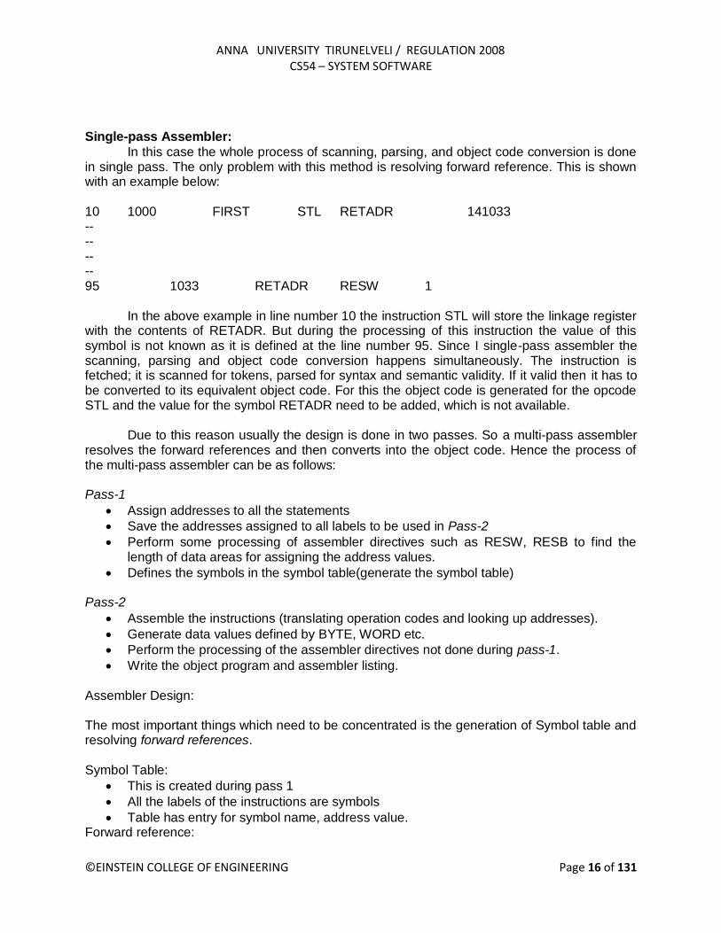
Single-pass Assembler:
In this case the whole process of scanning, parsing, and object code conversion is done in single pass. The only problem with this method is resolving forward reference. This is shown with an example below: 10 1000 FIRST STL RETADR 141033 -- -- -- -- 95 1033 RETADR RESW 1 In the above example in line number 10 the instruction STL will store the linkage register with the contents of RETADR. But during the processing of this instruction the value of this symbol is not known as it is defined at the line number 95. Since I single-pass assembler the scanning, parsing and object code conversion happens simultaneously. The instruction is fetched; it is scanned for tokens, parsed for syntax and semantic validity. If it valid then it has to be converted to its equivalent object code. For this the object code is generated for the opcode STL and the value for the symbol RETADR need to be added, which is not available. Due to this reason usually the design is done in two passes. So a multi-pass assembler resolves the forward references and then converts into the object code. Hence the process of the multi-pass assembler can be as follows: Pass-1
Assign addresses to all the statements
Save the addresses assigned to all labels to be used in Pass-2
Perform some processing of assembler directives such as RESW, RESB to find the length of data areas for assigning the address values.
Defines the symbols in the symbol table(generate the symbol table) Pass-2
Assemble the instructions (translating operation codes and looking up addresses).
Generate data values defined by BYTE, WORD etc.
Perform the processing of the assembler directives not done during pass-1.
Write the object program and assembler listing. Assembler Design: The most important things which need to be concentrated is the generation of Symbol table and resolving forward references.
Symbol Table:
This is created during pass 1
All the labels of the instructions are symbols
Table has entry for symbol name, address value. Forward reference:

ANNA UNIVERSITY TIRUNELVELI / REGULATION 2008 CS54 – SYSTEM SOFTWARE
©EINSTEIN COLLEGE OF ENGINEERING Page 17 of 131
Symbols that are defined in the later part of the program are called forward referencing.
There will not be any address value for such symbols in the symbol table in pass 1. Example Program: The example program considered here has a main module, two subroutines Purpose of example program
Reads records from input device (code F1)
Copies them to output device (code 05)
At the end of the file, writes EOF on the output device, then RSUB to the OS Data transfer (RD, WD)
A buffer is used to store record
Buffering is necessary for different I/O rates
The end of each record is marked with a null character (00)16
The end of the file is indicated by a zero-length record Subroutines (JSUB, RSUB)
RDREC, WRREC
Save link register first before nested jump

ANNA UNIVERSITY TIRUNELVELI / REGULATION 2008 CS54 – SYSTEM SOFTWARE
©EINSTEIN COLLEGE OF ENGINEERING Page 18 of 131

ANNA UNIVERSITY TIRUNELVELI / REGULATION 2008 CS54 – SYSTEM SOFTWARE
©EINSTEIN COLLEGE OF ENGINEERING Page 19 of 131

ANNA UNIVERSITY TIRUNELVELI / REGULATION 2008 CS54 – SYSTEM SOFTWARE
©EINSTEIN COLLEGE OF ENGINEERING Page 20 of 131
The first column shows the line number for that instruction, second column shows the addresses allocated to each instruction. The third column indicates the labels given to the statement, and is followed by the instruction consisting of opcode and operand. The last column gives the equivalent object code. The object code later will be loaded into memory for execution. The simple object program we use contains three types of records: Header record
- Col. 1 H - Col. 2~7 Program name - Col. 8~13 Starting address of object program (hex) - Col. 14~19 Length of object program in bytes (hex)
Text record - Col. 1 T - Col. 2~7 Starting address for object code in this record (hex) - Col. 8~9 Length of object code in this record in bytes (hex) - Col. 10~69 Object code, represented in hex (2 col. per byte)
End record - Col.1 E
Col.2~7 Address of first executable instruction in object program (hex) “^” is only for separation only Simple SIC Assembler The program below is shown with the object code generated. The column named LOC gives the machine addresses of each part of the assembled program (assuming the program is starting at location 1000). The translation of the source program to the object program requires us to accomplish the following functions:
Convert the mnemonic operation codes to their machine language equivalent.

ANNA UNIVERSITY TIRUNELVELI / REGULATION 2008 CS54 – SYSTEM SOFTWARE
©EINSTEIN COLLEGE OF ENGINEERING Page 21 of 131
Convert symbolic operands to their equivalent machine addresses.
Build the machine instructions in the proper format.
Convert the data constants specified in the source program into their internal machine representations in the proper format.
Write the object program and assembly listing. All these steps except the second can be performed by sequential processing of the source program, one line at a time. Consider the instruction 10 1000 LDA ALPHA 00----- This instruction contains the forward reference, i.e. the symbol ALPHA is used is not yet defined. If the program is processed ( scanning and parsing and object code conversion) is done line-by-line, we will be unable to resolve the address of this symbol. Due to this problem most of the assemblers are designed to process the program in two passes. In addition to the translation to object program, the assembler has to take care of handling assembler directive. These directives do not have object conversion but gives direction to the assembler to perform some function. Examples of directives are the statements like BYTE and WORD, which directs the assembler to reserve memory locations without generating data values. The other directives are START which indicates the beginning of the program and END indicating the end of the program. The assembled program will be loaded into memory for execution. The simple object program contains three types of records: Header record, Text record and end record. The header record contains the starting address and length. Text record contains the translated instructions and data of the program, together with an indication of the addresses where these are to be loaded. The end record marks the end of the object program and specifies the address where the execution is to begin. The format of each record is as given below. Header record: Col 1 H Col. 2-7 Program name Col 8-13 Starting address of object program (hexadecimal) Col 14-19 Length of object program in bytes (hexadecimal) Text record: Col. 1 T Col 2-7. Starting address for object code in this record (hexadecimal) Col 8-9 Length off object code in this record in bytes (hexadecimal) Col 10-69 Object code, represented in hexadecimal (2 columns per byte of object code) End record: Col. 1 E Col 2-7 Address of first executable instruction in object program (hexadecimal)

ANNA UNIVERSITY TIRUNELVELI / REGULATION 2008 CS54 – SYSTEM SOFTWARE
©EINSTEIN COLLEGE OF ENGINEERING Page 22 of 131
The assembler can be designed either as a single pass assembler or as a two pass assembler. The general description of both passes is as given below: Pass 1 (define symbols)
Assign addresses to all statements in the program
Save the addresses assigned to all labels for use in Pass 2
Perform assembler directives, including those for address assignment, such as BYTE and RESW
Pass 2 (assemble instructions and generate object program)
Assemble instructions (generate opcode and look up addresses)
Generate data values defined by BYTE, WORD
Perform processing of assembler directives not done during Pass 1
Write the object program and the assembly listing ALGORITHMS AND DATA STRUCTURE
The simple assembler uses two major internal data structures: the operation Code Table (OPTAB) and the Symbol Table (SYMTAB). OPTAB: It is used to lookup mnemonic operation codes and translates them to their machine language equivalents. In more complex assemblers the table also contains information about instruction format and length. In pass 1 the OPTAB is used to look up and validate the operation code in the source program. In pass 2, it is used to translate the operation codes to machine language. In simple SIC machine this process can be performed in either in pass 1 or in pass 2. But for machine like SIC/XE that has instructions of different lengths, we must search OPTAB in the first pass to find the instruction length for incrementing LOCCTR. In pass 2 we take the information from OPTAB to tell us which instruction format to use in assembling the instruction, and any peculiarities of the object code instruction. OPTAB is usually organized as a hash table, with mnemonic operation code as the key. The hash table organization is particularly appropriate, since it provides fast retrieval with a minimum of searching. Most of the cases the OPTAB is a static table- that is, entries are not normally added to or deleted from it. In such cases it is possible to design a special hashing function or other data structure to give optimum performance for the particular set of keys being stored. SYMTAB: This table includes the name and value for each label in the source program, together with flags to indicate the error conditions (e.g., if a symbol is defined in two different places). During Pass 1: labels are entered into the symbol table along with their assigned address value as they are encountered. All the symbols address value should get resolved at the pass 1. During Pass 2: Symbols used as operands are looked up the symbol table to obtain the address value to be inserted in the assembled instructions. SYMTAB is usually organized as a hash table for efficiency of insertion and retrieval. Since entries are rarely deleted, efficiency of deletion is the important criteria for optimization.
ANNA UNIVERSITY TIRUNELVELI / REGULATION 2008 CS54 – SYSTEM SOFTWARE
©EINSTEIN COLLEGE OF ENGINEERING Page 23 of 131
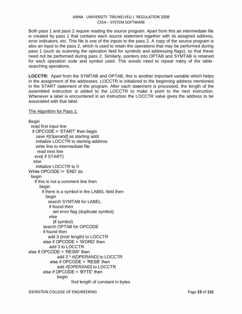
Both pass 1 and pass 2 require reading the source program. Apart from this an intermediate file is created by pass 1 that contains each source statement together with its assigned address, error indicators, etc. This file is one of the inputs to the pass 2. A copy of the source program is also an input to the pass 2, which is used to retain the operations that may be performed during pass 1 (such as scanning the operation field for symbols and addressing flags), so that these need not be performed during pass 2. Similarly, pointers into OPTAB and SYMTAB is retained for each operation code and symbol used. This avoids need to repeat many of the table-searching operations. LOCCTR: Apart from the SYMTAB and OPTAB, this is another important variable which helps
in the assignment of the addresses. LOCCTR is initialized to the beginning address mentioned in the START statement of the program. After each statement is processed, the length of the assembled instruction is added to the LOCCTR to make it point to the next instruction. Whenever a label is encountered in an instruction the LOCCTR value gives the address to be associated with that label. The Algorithm for Pass 1: Begin read first input line if OPCODE = „START‟ then begin save #[Operand] as starting addr initialize LOCCTR to starting address write line to intermediate file read next line end( if START) else initialize LOCCTR to 0 While OPCODE != „END‟ do begin if this is not a comment line then begin if there is a symbol in the LABEL field then begin search SYMTAB for LABEL if found then set error flag (duplicate symbol) else (if symbol) search OPTAB for OPCODE if found then add 3 (instr length) to LOCCTR else if OPCODE = „WORD‟ then add 3 to LOCCTR else if OPCODE = „RESW‟ then add 3 * #[OPERAND] to LOCCTR else if OPCODE = „RESB‟ then add #[OPERAND] to LOCCTR else if OPCODE = „BYTE‟ then begin find length of constant in bytes

ANNA UNIVERSITY TIRUNELVELI / REGULATION 2008 CS54 – SYSTEM SOFTWARE
©EINSTEIN COLLEGE OF ENGINEERING Page 24 of 131
add length to LOCCTR end else set error flag (invalid operation code) end (if not a comment) write line to intermediate file read next input line end { while not END} write last line to intermediate file Save (LOCCTR – starting address) as program length End {pass 1} The algorithm scans the first statement START and saves the operand field (the address) as the starting address of the program. Initializes the LOCCTR value to this address. This line is written to the intermediate line. If no operand is mentioned the LOCCTR is initialized to zero. If a label is encountered, the symbol has to be entered in the symbol table along with its associated address value. If the symbol already exists that indicates an entry of the same symbol already exists. So an error flag is set indicating a duplication of the symbol. It next checks for the mnemonic code, it searches for this code in the OPTAB. If found then the length of the instruction is added to the LOCCTR to make it point to the next instruction. If the opcode is the directive WORD it adds a value 3 to the LOCCTR. If it is RESW, it needs to add the number of data word to the LOCCTR. If it is BYTE it adds a value one to the LOCCTR, if RESB it adds number of bytes. If it is END directive then it is the end of the program it finds the length of the program by evaluating current LOCCTR – the starting address mentioned in the operand field of the END directive. Each processed line is written to the intermediate file. The Algorithm for Pass 2: Begin read 1st input line if OPCODE = „START‟ then begin write listing line read next input line end write Header record to object program initialize 1st Text record while OPCODE != „END‟ do begin if this is not comment line then begin search OPTAB for OPCODE if found then begin if there is a symbol in OPERAND field then begin search SYMTAB for OPERAND field then if found then begin

ANNA UNIVERSITY TIRUNELVELI / REGULATION 2008 CS54 – SYSTEM SOFTWARE
©EINSTEIN COLLEGE OF ENGINEERING Page 25 of 131
store symbol value as operand address else begin store 0 as operand address set error flag (undefined symbol) end end (if symbol) else store 0 as operand address assemble the object code instruction else if OPCODE = „BYTE‟ or „WORD” then convert constant to object code if object code doesn‟t fit into current Text record then begin Write text record to object code initialize new Text record end add object code to Text record end {if not comment} write listing line read next input line end write listing line read next input line write last listing line End {Pass 2} Here the first input line is read from the intermediate file. If the opcode is START, then this line is directly written to the list file. A header record is written in the object program which gives the starting address and the length of the program (which is calculated during pass 1). Then the first text record is initialized. Comment lines are ignored. In the instruction, for the opcode the OPTAB is searched to find the object code. If a symbol is there in the operand field, the symbol table is searched to get the address value for this which gets added to the object code of the opcode. If the address not found then zero value is stored as operands address. An error flag is set indicating it as undefined. If symbol itself is not found then store 0 as operand address and the object code instruction is assembled. If the opcode is BYTE or WORD, then the constant value is converted to its equivalent object code( for example, for character EOF, its equivalent hexadecimal value „454f46‟ is stored). If the object code cannot fit into the current text record, a new text record is created and the rest of the instructions object code is listed. The text records are written to the object program. Once the whole program is assemble and when the END directive is encountered, the End record is written.
DESIGN AND IMPLEMENTATION ISSUES Some of the features in the program depend on the architecture of the machine. If the program is for SIC machine, then we have only limited instruction formats and hence limited addressing modes. We have only single operand instructions. The operand is always a memory reference. Anything to be fetched from memory requires more time. Hence the improved version of SIC/XE

ANNA UNIVERSITY TIRUNELVELI / REGULATION 2008 CS54 – SYSTEM SOFTWARE
©EINSTEIN COLLEGE OF ENGINEERING Page 26 of 131
machine provides more instruction formats and hence more addressing modes. The moment we change the machine architecture, the availability of number of instruction formats and the addressing modes change. Therefore the design usually requires considering two things: Machine-dependent features and Machine-independent features. MACHINE-DEPENDENT FEATURES:
Instruction formats and addressing modes
Program relocation Instruction formats and Addressing Modes
The instruction formats depend on the memory organization and the size of the memory. In SIC machine the memory is byte addressable. Word size is 3 bytes. So the size of the memory is 212 bytes. Accordingly it supports only one instruction format. It has only two registers: register A and Index register. Therefore the addressing modes supported by this architecture are direct, indirect, and indexed. Whereas the memory of a SIC/XE machine is 220
bytes (1 MB). This supports four different types of instruction types, they are: 1 byte instruction 2 byte instruction 3 byte instruction 4 byte instruction
Instructions can be:
Instructions involving register to register
Instructions with one operand in memory, the other in Accumulator (Single operand instruction)
Extended instruction format Addressing Modes are:
Index Addressing(SIC): Opcode m, x Indirect Addressing: Opcode @m PC-relative: Opcode m Base relative: Opcode m Immediate addressing: Opcode #c
Translations for the Instruction involving Register-Register addressing mode:
During pass 1 the registers can be entered as part of the symbol table itself. The value for these registers is their equivalent numeric codes. During pass 2, these values are assembled along with the mnemonics object code. If required a separate table can be created with the register names and their equivalent numeric values. Translation involving Register-Memory instructions:
In SIC/XE machine there are four instruction formats and five addressing modes. For formats and addressing modes refer chapter 1. Among the instruction formats, format -3 and format-4 instructions are Register-Memory type of instruction. One of the operand is always in a register and the other operand is in the memory. The addressing mode tells us the way in which the operand from the memory is to be fetched. There are two ways: Program-counter relative and Base-relative. This addressing mode can be represented by either using format-3 type or format-4 type of instruction format. In format-3, the instruction has the opcode followed by a 12-bit displacement value in the address

ANNA UNIVERSITY TIRUNELVELI / REGULATION 2008 CS54 – SYSTEM SOFTWARE
©EINSTEIN COLLEGE OF ENGINEERING Page 27 of 131
field. Where as in format-4 the instruction contains the mnemonic code followed by a 20-bit displacement value in the address field. Program-Counter Relative:
In this usually format-3 instruction format is used. The instruction contains the opcode followed by a 12-bit displacement value. The range of displacement values are from 0 -2048. This displacement (should be small enough to fit in a 12-bit field) value is added to the current contents of the program counter to get the target address of the operand required by the instruction. This is relative way of calculating the address of the operand relative to the program counter. Hence the displacement of the operand is relative to the current program counter value. The following example shows how the address is calculated:
Base-Relative Addressing Mode: In this mode the base register is used to mention the displacement value. Therefore the target address is TA = (base) + displacement value This addressing mode is used when the range of displacement value is not sufficient. Hence the operand is not relative to the instruction as in PC-relative addressing mode. Whenever this mode is used it is indicated by using a directive BASE. The moment the assembler encounters this directive the next instruction uses base-relative addressing mode to calculate the target address of the operand. When NOBASE directive is used then it indicates the base register is no more used to calculate the target address of the operand. Assembler first chooses PC-relative, when the displacement field is not enough it uses Base-relative. LDB #LENGTH (instruction)
ANNA UNIVERSITY TIRUNELVELI / REGULATION 2008 CS54 – SYSTEM SOFTWARE
©EINSTEIN COLLEGE OF ENGINEERING Page 28 of 131
BASE LENGTH (directive)
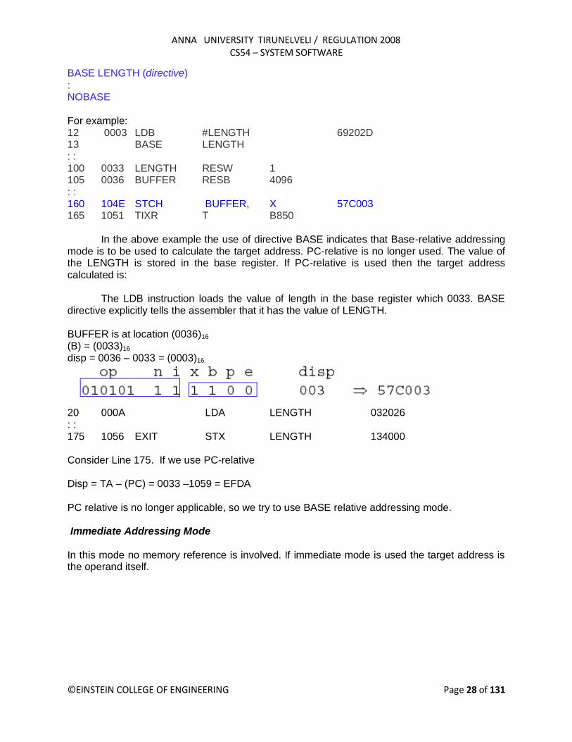
: NOBASE For example: 12 0003 LDB #LENGTH 69202D 13 BASE LENGTH : : 100 0033 LENGTH RESW 1 105 0036 BUFFER RESB 4096 : : 160 104E STCH BUFFER, X 57C003 165 1051 TIXR T B850 In the above example the use of directive BASE indicates that Base-relative addressing mode is to be used to calculate the target address. PC-relative is no longer used. The value of the LENGTH is stored in the base register. If PC-relative is used then the target address calculated is: The LDB instruction loads the value of length in the base register which 0033. BASE directive explicitly tells the assembler that it has the value of LENGTH. BUFFER is at location (0036)16 (B) = (0033)16 disp = 0036 – 0033 = (0003)16
20 000A LDA LENGTH 032026 : : 175 1056 EXIT STX LENGTH 134000 Consider Line 175. If we use PC-relative Disp = TA – (PC) = 0033 –1059 = EFDA PC relative is no longer applicable, so we try to use BASE relative addressing mode. Immediate Addressing Mode In this mode no memory reference is involved. If immediate mode is used the target address is the operand itself.

ANNA UNIVERSITY TIRUNELVELI / REGULATION 2008 CS54 – SYSTEM SOFTWARE
©EINSTEIN COLLEGE OF ENGINEERING Page 29 of 131
If the symbol is referred in the instruction as the immediate operand then it is immediate with PC-relative mode as shown in the example below:
5. Indirect and PC-relative mode:
In this type of instruction the symbol used in the instruction is the address of the location which contains the address of the operand. The address of this is found using PC-relative addressing mode. For example:
The instruction jumps the control to the address location RETADR which in turn has the address of the operand. If address of RETADR is 0030, the target address is then 0003 as calculated above. Program Relocation

ANNA UNIVERSITY TIRUNELVELI / REGULATION 2008 CS54 – SYSTEM SOFTWARE
©EINSTEIN COLLEGE OF ENGINEERING Page 30 of 131
Sometimes it is required to load and run several programs at the same time. The system must be able to load these programs wherever there is place in the memory. Therefore the exact starting is not known until the load time. Absolute Program In this the address is mentioned during assembling itself. This is called Absolute Assembly.
Consider the instruction: 55 101B LDA THREE 00102D This statement says that the register A is loaded with the value stored at location 102D. Suppose it is decided to load and execute the program at location 2000 instead of location 1000. Then at address 102D the required value which needs to be loaded in the register A is no more available. The address also gets changed relative to the displacement of the program. Hence we need to make some changes in the address portion of the instruction so that we can load and execute the program at location 2000. Apart from the instruction which will undergo a change in their operand address value as the program load address changes. There exist some parts in the program which will remain same regardless of where the program is being loaded. Since assembler will not know actual location where the program will get loaded, it cannot make the necessary changes in the addresses used in the program. However, the assembler identifies for the loader those parts of the program which need modification. An object program that has the information necessary to perform this kind of modification is called the relocatable program.
The above diagram shows the concept of relocation. Initially the program is loaded at location 0000. The instruction JSUB is loaded at location 0006. The address field of this instruction contains 01036, which is the address of the instruction labeled RDREC. The second figure shows that if the program is to be loaded at new location 5000. The address of the instruction JSUB gets modified to new location 6036. Likewise the third figure shows that if the program is relocated at location 7420, the JSUB instruction would need to be changed to 4B108456 that correspond to the new address of RDREC.

ANNA UNIVERSITY TIRUNELVELI / REGULATION 2008 CS54 – SYSTEM SOFTWARE
©EINSTEIN COLLEGE OF ENGINEERING Page 31 of 131
The only part of the program that require modification at load time are those that specify direct addresses. The rest of the instructions need not be modified. The instructions which doesn‟t require modification are the ones that is not a memory address (immediate addressing) and PC-relative, Base-relative instructions. From the object program, it is not possible to distinguish the address and constant The assembler must keep some information to tell the loader. The object program that contains the modification record is called a relocatable program. For an address label, its address is assigned relative to the start of the program (START 0). The assembler produces a Modification record to store the starting location and the length of the
address field to be modified. The command for the loader must also be a part of the object program. The Modification has the following format: Modification record Col. 1 M Col. 2-7 Starting location of the address field to be modified, relative to the beginning of the program (Hex) Col. 8-9 Length of the address field to be modified, in half-bytes (Hex) One modification record is created for each address to be modified The length is stored in half-bytes (4 bits) The starting location is the location of the byte containing the leftmost bits of the address field to be modified. If the field contains an odd number of half-bytes, the starting location begins in the middle of the first byte.
In the above object code the red boxes indicate the addresses that need modifications. The object code lines at the end are the descriptions of the modification records for those instructions which need change if relocation occurs. M00000705 is the modification suggested for the statement at location 0007 and requires modification 5-half bytes. Similarly the remaining instructions indicate. Machine-Independent features: These are the features which do not depend on the architecture of the machine. These are:
Literals
Expressions
Program blocks
Control sections

ANNA UNIVERSITY TIRUNELVELI / REGULATION 2008 CS54 – SYSTEM SOFTWARE
©EINSTEIN COLLEGE OF ENGINEERING Page 32 of 131
Literals: A literal is defined with a prefix = followed by a specification of the literal value. Example: 45 001A ENDFIL LDA =C‟EOF‟ 032010 - - 93 LTORG 002D * =C‟EOF‟ 454F46 The example above shows a 3-byte operand whose value is a character string EOF. The object code for the instruction is also mentioned. It shows the relative displacement value of the location where this value is stored. In the example the value is at location (002D) and hence the displacement value is (010). As another example the given statement below shows a 1-byte literal with the hexadecimal value „05‟. 215 1062 WLOOP TD =X‟05‟ E32011 It is important to understand the difference between a constant defined as a literal and a constant defined as an immediate operand. In case of literals the assembler generates the specified value as a constant at some other memory location In immediate mode the operand value is assembled as part of the instruction itself. Example 55 0020 LDA #03 010003 All the literal operands used in a program are gathered together into one or more literal pools. This is usually placed at the end of the program. The assembly listing of a program
containing literals usually includes a listing of this literal pool, which shows the assigned addresses and the generated data values. In some cases it is placed at some other location in the object program. An assembler directive LTORG is used. Whenever the LTORG is encountered, it creates a literal pool that contains all the literal operands used since the beginning of the program. The literal pool definition is done after LTORG is encountered. It is better to place the literals close to the instructions. A literal table is created for the literals which are used in the program. The literal table contains the literal name, operand value and length. The literal table is usually created as a hash table on the literal name. Implementation of Literals: During Pass-1:
The literal encountered is searched in the literal table. If the literal already exists, no action is taken; if it is not present, the literal is added to the LITTAB and for the address value it waits till it encounters LTORG for literal definition. When Pass 1 encounters a LTORG statement or the end of the program, the assembler makes a scan of the literal table. At this time each literal currently in the table is assigned an address. As addresses are assigned, the location counter is updated to reflect the number of bytes occupied by each literal. During Pass-2:

ANNA UNIVERSITY TIRUNELVELI / REGULATION 2008 CS54 – SYSTEM SOFTWARE
©EINSTEIN COLLEGE OF ENGINEERING Page 33 of 131
The assembler searches the LITTAB for each literal encountered in the instruction and replaces it with its equivalent value as if these values are generated by BYTE or WORD. If a literal represents an address in the program, the assembler must generate a modification relocation for, if it all it gets affected due to relocation. The following figure shows the difference between the SYMTAB and LITTAB
Symbol-Defining Statements:
EQU Statement: Most assemblers provide an assembler directive that allows the programmer to define symbols and specify their values. The directive used for this EQU (Equate). The general form of the statement is Symbol EQU value This statement defines the given symbol (i.e., entering in the SYMTAB) and assigning to it the value specified. The value can be a constant or an expression involving constants and any other symbol which is already defined. One common usage is to define symbolic names that can be used to improve readability in place of numeric values. For example +LDT #4096 This loads the register T with immediate value 4096, this does not clearly what exactly this value indicates. If a statement is included as: MAXLEN EQU 4096 and then +LDT #MAXLEN Then it clearly indicates that the value of MAXLEN is some maximum length value. When the assembler encounters EQU statement, it enters the symbol MAXLEN along with its value in the symbol table. During LDT the assembler searches the SYMTAB for its entry and its equivalent value as the operand in the instruction. The object code generated is the same for both the options discussed, but is easier to understand. If the maximum length is changed from 4096 to 1024, it is difficult to change if it is mentioned as an immediate value wherever required in the instructions. We have to scan the whole program and make changes wherever 4096 is used. If we mention this value in the instruction through the symbol defined by EQU, we may not have to search the whole program but change only the value of MAXLENGTH in the EQU statement (only once).

ANNA UNIVERSITY TIRUNELVELI / REGULATION 2008 CS54 – SYSTEM SOFTWARE
©EINSTEIN COLLEGE OF ENGINEERING Page 34 of 131
Another common usage of EQU statement is for defining values for the general-purpose registers. The assembler can use the mnemonics for register usage like a-register A , X – index register and so on. But there are some instructions which requires numbers in place of names in the instructions. For example in the instruction RMO 0,1 instead of RMO A,X. The programmer can assign the numerical values to these registers using EQU directive. A EQU 0 X EQU 1 and so on These statements will cause the symbols A, X, L… to be entered into the symbol table with their respective values. An instruction RMO A, X would then be allowed. As another usage if in a machine that has many general purpose registers named as R1, R2,…, some may be used as base register, some may be used as accumulator. Their usage may change from one program to another. In this case we can define these requirement using EQU statements. BASE EQU R1 INDEX EQU R2 COUNT EQU R3 One restriction with the usage of EQU is whatever symbol occurs in the right hand side of the EQU should be predefined. For example, the following statement is not valid: BETA EQU ALPHA ALPHA RESW 1 As the symbol ALPHA is assigned to BETA before it is defined. The value of ALPHA is not known. ORG Statement:
This directive can be used to indirectly assign values to the symbols. The directive is usually called ORG (for origin). Its general format is: ORG value where value is a constant or an expression involving constants and previously defined symbols. When this statement is encountered during assembly of a program, the assembler resets its location counter (LOCCTR) to the specified value. Since the values of symbols used as labels are taken from LOCCTR, the ORG statement will affect the values of all labels defined until the next ORG is encountered. ORG is used to control assignment storage in the object program. Sometimes altering the values may result in incorrect assembly. ORG can be useful in label definition. Suppose we need to define a symbol table with the following structure: SYMBOL 6 Bytes VALUE 3 Bytes FLAG 2 Bytes The table looks like the one given below.

ANNA UNIVERSITY TIRUNELVELI / REGULATION 2008 CS54 – SYSTEM SOFTWARE
©EINSTEIN COLLEGE OF ENGINEERING Page 35 of 131
The symbol field contains a 6-byte user-defined symbol; VALUE is a one-word representation of the value assigned to the symbol; FLAG is a 2-byte field specifies symbol type and other information. The space for the ttable can be reserved by the statement: STAB RESB 1100 If we want to refer to the entries of the table using indexed addressing, place the offset value of the desired entry from the beginning of the table in the index register. To refer to the fields SYMBOL, VALUE, and FLAGS individually, we need to assign the values first as shown below: SYMBOL EQU STAB VALUE EQU STAB+6 FLAGS EQU STAB+9 To retrieve the VALUE field from the table indicated by register X, we can write a statement: LDA VALUE, X The same thing can also be done using ORG statement in the following way: STAB RESB 1100 ORG STAB SYMBOL RESB 6 VALUE RESW 1 FLAG RESB 2 ORG STAB+1100 The first statement allocates 1100 bytes of memory assigned to label STAB. In the second statement the ORG statement initializes the location counter to the value of STAB. Now the LOCCTR points to STAB. The next three lines assign appropriate memory storage to each of SYMBOL, VALUE and FLAG symbols. The last ORG statement reinitializes the LOCCTR to a new value after skipping the required number of memory for the table STAB (i.e., STAB+1100).

ANNA UNIVERSITY TIRUNELVELI / REGULATION 2008 CS54 – SYSTEM SOFTWARE
©EINSTEIN COLLEGE OF ENGINEERING Page 36 of 131
While using ORG, the symbol occurring in the statement should be predefined as is required in EQU statement. For example for the sequence of statements below: ORG ALPHA BYTE1 RESB 1 BYTE2 RESB 1 BYTE3 RESB 1 ORG ALPHA RESB 1 The sequence could not be processed as the symbol used to assign the new location counter value is not defined. In first pass, as the assembler would not know what value to assign to ALPHA, the other symbol in the next lines also could not be defined in the symbol table. This is a kind of problem of the forward reference. EXPRESSIONS: Assemblers also allow use of expressions in place of operands in the instruction. Each such expression must be evaluated to generate a single operand value or address. Assemblers generally arithmetic expressions formed according to the normal rules using arithmetic operators +, - *, /. Division is usually defined to produce an integer result. Individual terms may be constants, user-defined symbols, or special terms. The only special term used is * ( the current value of location counter) which indicates the value of the next unassigned memory location. Thus the statement BUFFEND EQU * Assigns a value to BUFFEND, which is the address of the next byte following the buffer area. Some values in the object program are relative to the beginning of the program and some are absolute (independent of the program location, like constants). Hence, expressions are classified as either absolute expression or relative expressions depending on the type of value they produce. Absolute Expressions: The expression that uses only absolute terms is absolute expression.
Absolute expression may contain relative term provided the relative terms occur in pairs with opposite signs for each pair. Example: MAXLEN EQU BUFEND-BUFFER In the above instruction the difference in the expression gives a value that does not depend on the location of the program and hence gives an absolute immaterial o the relocation of the program. The expression can have only absolute terms. Example: MAXLEN EQU 1000 Relative Expressions: All the relative terms except one can be paired as described in “absolute”. The remaining unpaired relative term must have a positive sign. Example: STAB EQU OPTAB + (BUFEND – BUFFER)

ANNA UNIVERSITY TIRUNELVELI / REGULATION 2008 CS54 – SYSTEM SOFTWARE
©EINSTEIN COLLEGE OF ENGINEERING Page 37 of 131
Handling the type of expressions: to find the type of expression, we must keep track the type of symbols used. This can be achieved by defining the type in the symbol table against each of the symbol as shown in the table below:
Program Blocks:
Program blocks allow the generated machine instructions and data to appear in the object program in a different order by Separating blocks for storing code, data, stack, and larger data block. Assembler Directive USE:
USE [blockname] At the beginning, statements are assumed to be part of the unnamed (default) block. If no USE
statements are included, the entire program belongs to this single block. Each program block may actually contain several separate segments of the source program. Assemblers rearrange these segments to gather together the pieces of each block and assign address. Separate the program into blocks in a particular order. Large buffer area is moved to the end of the object program. Program readability is better if data areas are placed in the source program close to the statements that reference them. In the example below three blocks are used :
Default: executable instructions CDATA: all data areas that are less in length CBLKS: all data areas that consists of larger blocks of memory
Example Code

ANNA UNIVERSITY TIRUNELVELI / REGULATION 2008 CS54 – SYSTEM SOFTWARE
©EINSTEIN COLLEGE OF ENGINEERING Page 38 of 131

ANNA UNIVERSITY TIRUNELVELI / REGULATION 2008 CS54 – SYSTEM SOFTWARE
©EINSTEIN COLLEGE OF ENGINEERING Page 39 of 131
Arranging code into program blocks: Pass 1
A separate location counter for each program block is maintained. Save and restore LOCCTR when switching between blocks. At the beginning of a block, LOCCTR is set to 0. Assign each label an address relative to the start of the block. Store the block name or number in the SYMTAB along with the assigned relative address of the label Indicate the block length as the latest value of LOCCTR for each block at the end of Pass1 Assign to each block a starting address in the object program by concatenating the program blocks in a particular order
Pass 2 Calculate the address for each symbol relative to the start of the object program by adding The location of the symbol relative to the start of its block The starting address of this block
Control Sections:
A control section is a part of the program that maintains its identity after assembly; each control section can be loaded and relocated independently of the others. Different control sections are most often used for subroutines or other logical subdivisions. The programmer can assemble, load, and manipulate each of these control sections separately. Because of this, there should be some means for linking control sections together. For example, instructions in one control section may refer to the data or instructions of other control sections. Since control sections are independently loaded and relocated, the assembler is unable to process these references in the usual way. Such references between different control sections are called external references.

ANNA UNIVERSITY TIRUNELVELI / REGULATION 2008 CS54 – SYSTEM SOFTWARE
©EINSTEIN COLLEGE OF ENGINEERING Page 40 of 131
The assembler generates the information about each of the external references that will allow the loader to perform the required linking. When a program is written using multiple control sections, the beginning of each of the control section is indicated by an assembler directive assembler directive: CSECT The syntax
secname CSECT separate location counter for each control section Control sections differ from program blocks in that they are handled separately by the assembler. Symbols that are defined in one control section may not be used directly another control section; they must be identified as external reference for the loader to handle. The external references are indicated by two assembler directives: EXTDEF (external Definition): It is the statement in a control section, names symbols that are defined in this section but may be used by other control sections. Control section names do not need to be named in the EXTREF as they are automatically considered as external symbols. EXTREF (external Reference): It names symbols that are used in this section but are defined in some other control section. The order in which these symbols are listed is not significant. The assembler must include proper information about the external references in the object program that will cause the loader to insert the proper value where they are required.

ANNA UNIVERSITY TIRUNELVELI / REGULATION 2008 CS54 – SYSTEM SOFTWARE
©EINSTEIN COLLEGE OF ENGINEERING Page 41 of 131
Handling External Reference
Case 1 15 0003 CLOOP +JSUB RDREC 4B100000 The operand RDREC is an external reference. The assembler has no idea where RDREC is

ANNA UNIVERSITY TIRUNELVELI / REGULATION 2008 CS54 – SYSTEM SOFTWARE
©EINSTEIN COLLEGE OF ENGINEERING Page 42 of 131
inserts an address of zero can only use extended format to provide enough room (that is, relative addressing for external reference is invalid) The assembler generates information for each external reference that will allow the loader to perform the required linking. Case 2 190 0028 MAXLEN WORD BUFEND-BUFFER 000000 There are two external references in the expression, BUFEND and BUFFER. The assembler inserts a value of zero passes information to the loader Add to this data area the address of BUFEND Subtract from this data area the address of BUFFER Case 3 On line 107, BUFEND and BUFFER are defined in the same control section and the expression can be calculated immediately. 107 1000 MAXLEN EQU BUFEND-BUFFER Object Code for the example program:

ANNA UNIVERSITY TIRUNELVELI / REGULATION 2008 CS54 – SYSTEM SOFTWARE
©EINSTEIN COLLEGE OF ENGINEERING Page 43 of 131
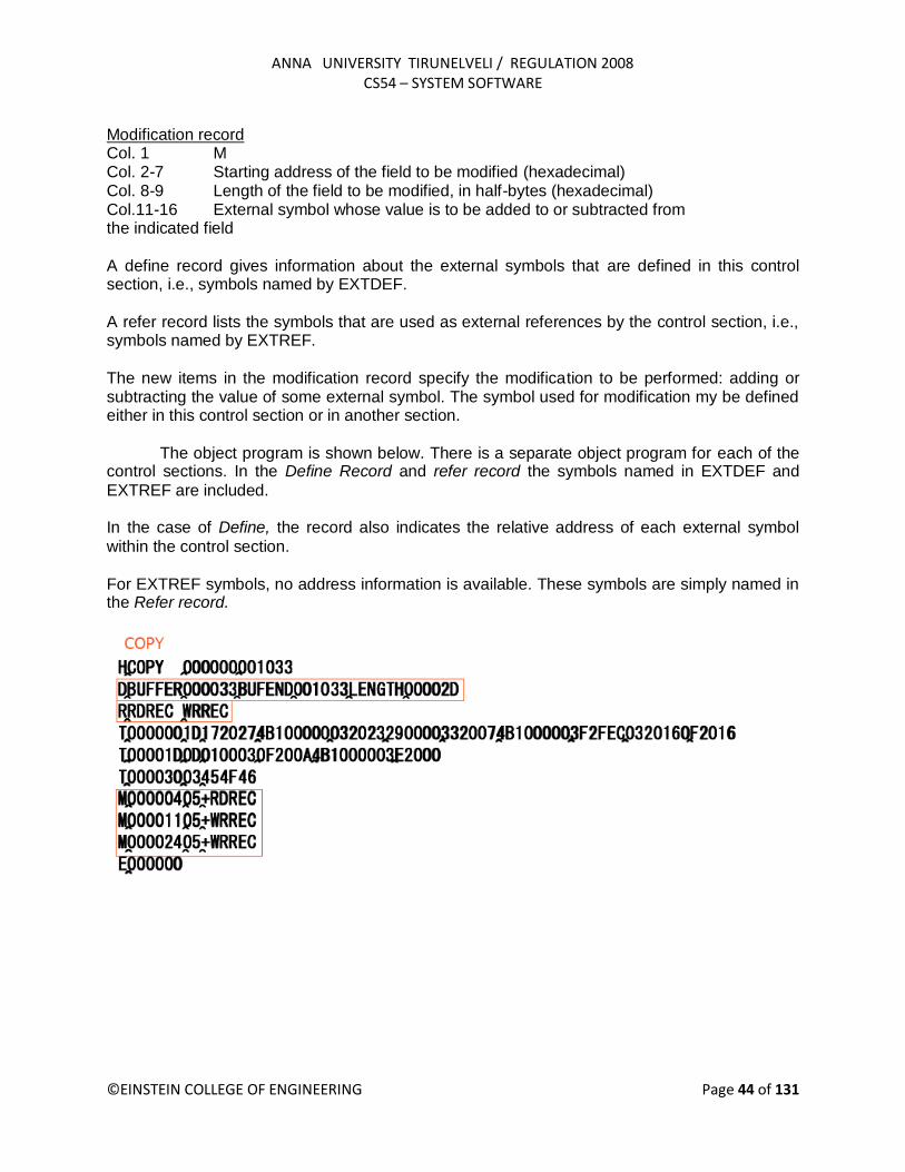
The assembler must also include information in the object program that will cause the loader to insert the proper value where they are required. The assembler maintains two new record in the object code and a changed version of modification record. Define record (EXTDEF) Col. 1 D Col. 2-7 Name of external symbol defined in this control section Col. 8-13 Relative address within this control section (hexadecimal) Col.14-73 Repeat information in Col. 2-13 for other external symbols Refer record (EXTREF) Col. 1 R Col. 2-7 Name of external symbol referred to in this control section Col. 8-73 Name of other external reference symbols
ANNA UNIVERSITY TIRUNELVELI / REGULATION 2008 CS54 – SYSTEM SOFTWARE
©EINSTEIN COLLEGE OF ENGINEERING Page 44 of 131
Modification record Col. 1 M Col. 2-7 Starting address of the field to be modified (hexadecimal) Col. 8-9 Length of the field to be modified, in half-bytes (hexadecimal) Col.11-16 External symbol whose value is to be added to or subtracted from the indicated field A define record gives information about the external symbols that are defined in this control section, i.e., symbols named by EXTDEF. A refer record lists the symbols that are used as external references by the control section, i.e., symbols named by EXTREF. The new items in the modification record specify the modification to be performed: adding or subtracting the value of some external symbol. The symbol used for modification my be defined either in this control section or in another section. The object program is shown below. There is a separate object program for each of the control sections. In the Define Record and refer record the symbols named in EXTDEF and
EXTREF are included. In the case of Define, the record also indicates the relative address of each external symbol
within the control section. For EXTREF symbols, no address information is available. These symbols are simply named in the Refer record.

ANNA UNIVERSITY TIRUNELVELI / REGULATION 2008 CS54 – SYSTEM SOFTWARE
©EINSTEIN COLLEGE OF ENGINEERING Page 45 of 131
Handling Expressions in Multiple Control Sections:
The existence of multiple control sections that can be relocated independently of one another makes the handling of expressions complicated. It is required that in an expression that all the relative terms be paired (for absolute expression), or that all except one be paired (for relative expressions). When it comes in a program having multiple control sections then we have an extended restriction that: Both terms in each pair of an expression must be within the same control section If two terms represent relative locations within the same control section , their difference is an absolute value (regardless of where the control section is located. Legal: BUFEND-BUFFER (both are in the same control section) If the terms are located in different control sections, their difference has a value that is unpredictable. Illegal: RDREC-COPY (both are of different control section) it is the difference in the load addresses of the two control sections. This value depends on the way run-time storage is allocated; it is unlikely to be of any use. How to enforce this restriction When an expression involves external references, the assembler cannot determine whether or not the expression is legal. The assembler evaluates all of the terms it can, combines these to form an initial expression value, and generates Modification records. The loader checks the expression for errors and finishes the evaluation. One-Pass Assembler

ANNA UNIVERSITY TIRUNELVELI / REGULATION 2008 CS54 – SYSTEM SOFTWARE
©EINSTEIN COLLEGE OF ENGINEERING Page 46 of 131
The main problem in designing the assembler using single pass was to resolve forward references. We can avoid to some extent the forward references by: Eliminating forward reference to data items, by defining all the storage reservation statements at the beginning of the program rather at the end. Unfortunately, forward reference to labels on the instructions cannot be avoided. (forward jumping) To provide some provision for handling forward references by prohibiting forward references to data items. There are two types of one-pass assemblers: One that produces object code directly in memory for immediate execution (Load-and-go assemblers). The other type produces the usual kind of object code for later execution. Load-and-Go Assembler
Load-and-go assembler generates their object code in memory for immediate execution. No object program is written out, no loader is needed. It is useful in a system with frequent program development and testing The efficiency of the assembly process is an important consideration. Programs are re-assembled nearly every time they are run; efficiency of the assembly process is an important consideration.
Forward Reference in One-Pass Assemblers: In load-and-Go assemblers when a forward reference is encountered :
ANNA UNIVERSITY TIRUNELVELI / REGULATION 2008 CS54 – SYSTEM SOFTWARE
©EINSTEIN COLLEGE OF ENGINEERING Page 47 of 131
Omits the operand address if the symbol has not yet been defined
Enters this undefined symbol into SYMTAB and indicates that it is undefined
Adds the address of this operand address to a list of forward references associated with the SYMTAB entry
When the definition for the symbol is encountered, scans the reference list and inserts the address.
At the end of the program, reports the error if there are still SYMTAB entries indicated undefined symbols.
For Load-and-Go assembler
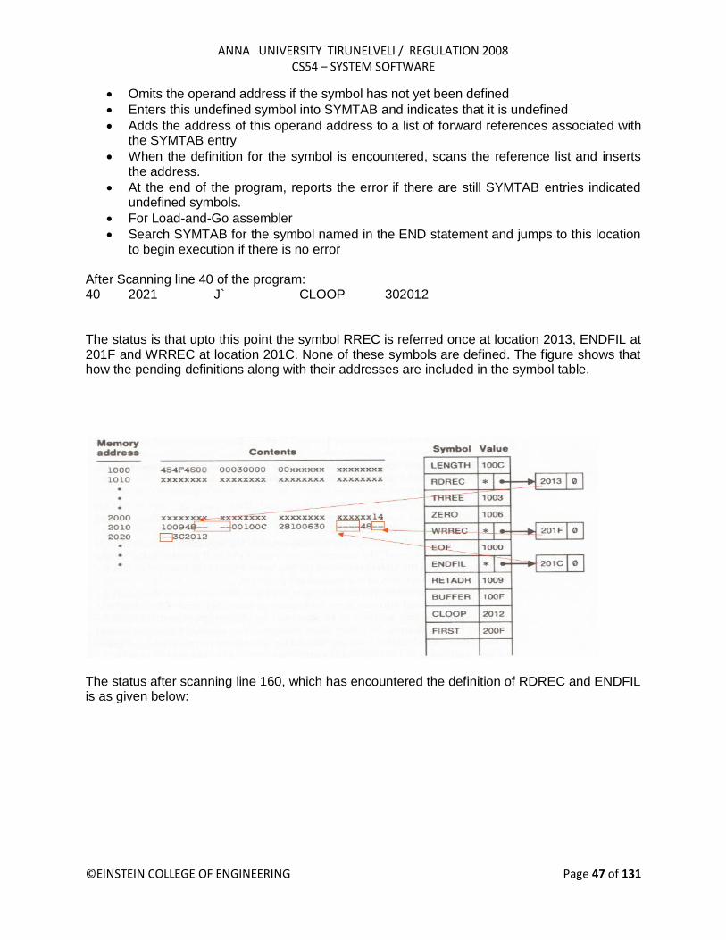
Search SYMTAB for the symbol named in the END statement and jumps to this location to begin execution if there is no error
After Scanning line 40 of the program: 40 2021 J` CLOOP 302012 The status is that upto this point the symbol RREC is referred once at location 2013, ENDFIL at 201F and WRREC at location 201C. None of these symbols are defined. The figure shows that how the pending definitions along with their addresses are included in the symbol table.
The status after scanning line 160, which has encountered the definition of RDREC and ENDFIL is as given below:

ANNA UNIVERSITY TIRUNELVELI / REGULATION 2008 CS54 – SYSTEM SOFTWARE
©EINSTEIN COLLEGE OF ENGINEERING Page 48 of 131
If One-Pass needs to generate object code:
If the operand contains an undefined symbol, use 0 as the address and write the Text record to the object program.
Forward references are entered into lists as in the load-and-go assembler.
When the definition of a symbol is encountered, the assembler generates another Text record with the correct operand address of each entry in the reference list.
When loaded, the incorrect address 0 will be updated by the latter Text record containing the symbol definition.
Object Code Generated by One-Pass Assembler:
Multi Pass Assembler:
For a two pass assembler, forward references in symbol definition are not allowed: ALPHA EQU BETA BETA EQU DELTA DELTA RESW 1 Symbol definition must be completed in pass 1. Prohibiting forward references in symbol definition is not a serious inconvenience. Forward references tend to create difficulty for a person reading the program. Implementation Issues for Modified Two-Pass Assembler: Implementation Issues when forward referencing is encountered in Symbol Defining statements
: For a forward reference in symbol definition, we store in the SYMTAB:

ANNA UNIVERSITY TIRUNELVELI / REGULATION 2008 CS54 – SYSTEM SOFTWARE
©EINSTEIN COLLEGE OF ENGINEERING Page 49 of 131
The symbol name, The defining expression, The number of undefined symbols in the defining expression, The undefined symbol (marked with a flag *) associated with a list of symbols depend on this undefined symbol. When a symbol is defined, we can recursively evaluate the symbol expressions depending on the newly defined symbol. Multi-Pass Assembler Example Program
Multi-Pass Assembler (Figure 2.21 of Beck): Example for forward reference in Symbol Defining Statements:

ANNA UNIVERSITY TIRUNELVELI / REGULATION 2008 CS54 – SYSTEM SOFTWARE
©EINSTEIN COLLEGE OF ENGINEERING Page 50 of 131
UNIT III - LOADERS AND LINKERS
Introduction
The Source Program written in assembly language or high level language will be converted to object program, which is in the machine language form for execution. This conversion either from assembler or from compiler, contains translated instructions and data values from the source program, or specifies addresses in primary memory where these items are to be loaded for execution. This contains the following three processes, and they are,
Loading - which allocates memory location and brings the object program into memory
for execution - (Loader) Linking- which combines two or more separate object programs and supplies the
information needed to allow references between them - (Linker) Relocation - which modifies the object program so that it can be loaded at an address
different from the location originally specified - (Linking Loader) Basic Loader Functions
A loader is a system program that performs the loading function. It brings object program
into memory and starts its execution. The role of loader is as shown in the figure 3.1. In figure
3.1 translator may be assembler/complier, which generates the object program and later loaded
to the memory by the loader for execution. In figure 3.2 the translator is specifically an
assembler, which generates the object loaded, which becomes input to the loader. The figure
3.3 shows the role of both loader and linker.
Figure 3.1 : The Role of Loader
Translator
Object
Program
Loader
Object program ready for execution
Memory
Source Program
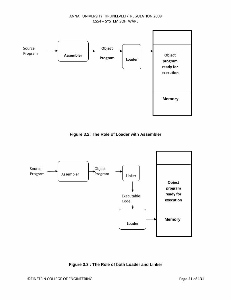
ANNA UNIVERSITY TIRUNELVELI / REGULATION 2008 CS54 – SYSTEM SOFTWARE
©EINSTEIN COLLEGE OF ENGINEERING Page 51 of 131
Figure 3.2: The Role of Loader with Assembler
Figure 3.3 : The Role of both Loader and Linker
Assembler
Object Program
Linker
Object
program
ready for
execution
Memory
Executable Code
Loader
Source Program
Assembler
Object
Program
Loader Object
program
ready for
execution
Memory
Source Program

ANNA UNIVERSITY TIRUNELVELI / REGULATION 2008 CS54 – SYSTEM SOFTWARE
©EINSTEIN COLLEGE OF ENGINEERING Page 52 of 131
Type of Loaders
The different types of loaders are, absolute loader, bootstrap loader, relocating loader
(relative loader), and, direct linking loader. The following sections discuss the functions and
design of all these types of loaders.
Absolute Loader
The operation of absolute loader is very simple. The object code is loaded to specified
locations in the memory. At the end the loader jumps to the specified address to begin
execution of the loaded program. The role of absolute loader is as shown in the figure 3.3.1.
The advantage of absolute loader is simple and efficient. But the disadvantages are, the need
for programmer to specify the actual address, and, difficult to use subroutine libraries.
Figure 3.3.1: The Role of Absolute Loader
The algorithm for this type of loader is given here. The object program and, the object
program loaded into memory by the absolute loader are also shown. Each byte of assembled
code is given using its hexadecimal representation in character form. Easy to read by human
beings. Each byte of object code is stored as a single byte. Most machine store object programs
in a binary form, and we must be sure that our file and device conventions do not cause some of
the program bytes to be interpreted as control characters.
Object Program
Absolute Loader
Object
program
ready for
execution
Memory
1000
2000

ANNA UNIVERSITY TIRUNELVELI / REGULATION 2008 CS54 – SYSTEM SOFTWARE
©EINSTEIN COLLEGE OF ENGINEERING Page 53 of 131
Begin read Header record verify program name and length read first Text record while record type is <> ‘E’ do begin {if object code is in character form, convert into internal representation} move object code to specified location in memory read next object program record end jump to address specified in End record end

ANNA UNIVERSITY TIRUNELVELI / REGULATION 2008 CS54 – SYSTEM SOFTWARE
©EINSTEIN COLLEGE OF ENGINEERING Page 54 of 131
A Simple Bootstrap Loader
When a computer is first turned on or restarted, a special type of absolute loader, called
bootstrap loader is executed. This bootstrap loads the first program to be run by the computer --
usually an operating system. The bootstrap itself begins at address 0. It loads the OS starting
address 0x80. No header record or control information, the object code is consecutive bytes of
memory.
The algorithm for the bootstrap loader is as follows
Begin X=0x80 (the address of the next memory location to be loaded Loop
AGETC (and convert it from the ASCII character code to the value of the hexadecimal digit) save the value in the high-order 4 bits of S
AGETC
combine the value to form one byte A (A+S) store the value (in A) to the address in register X
XX+1 End
It uses a subroutine GETC, which is
GETC Aread one character if A=0x04 then jump to 0x80 if A<48 then GETC
A A-48 (0x30) if A<10 then return
A A-7 return Machine-Dependent Loader Features
Absolute loader is simple and efficient, but the scheme has potential disadvantages One
of the most disadvantage is the programmer has to specify the actual starting address, from
where the program to be loaded. This does not create difficulty, if one program to run, but not
for several programs. Further it is difficult to use subroutine libraries efficiently.
This needs the design and implementation of a more complex loader. The loader must
provide program relocation and linking, as well as simple loading functions.
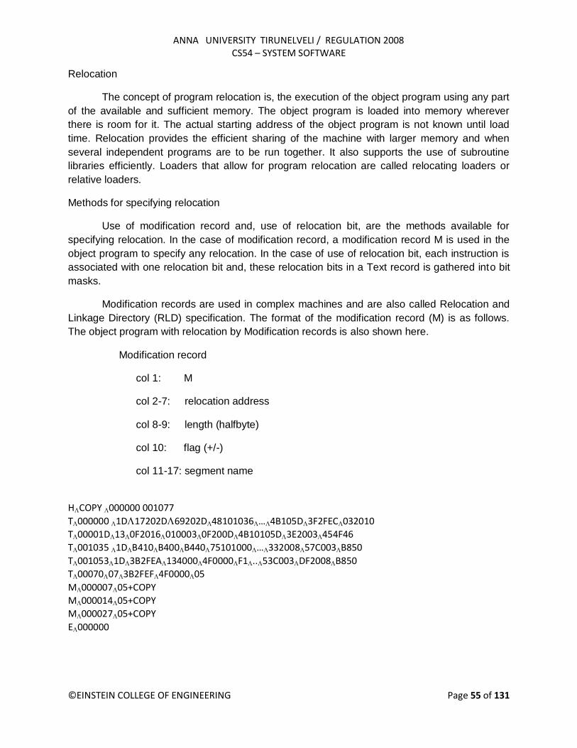
ANNA UNIVERSITY TIRUNELVELI / REGULATION 2008 CS54 – SYSTEM SOFTWARE
©EINSTEIN COLLEGE OF ENGINEERING Page 55 of 131
Relocation
The concept of program relocation is, the execution of the object program using any part
of the available and sufficient memory. The object program is loaded into memory wherever
there is room for it. The actual starting address of the object program is not known until load
time. Relocation provides the efficient sharing of the machine with larger memory and when
several independent programs are to be run together. It also supports the use of subroutine
libraries efficiently. Loaders that allow for program relocation are called relocating loaders or
relative loaders.
Methods for specifying relocation
Use of modification record and, use of relocation bit, are the methods available for
specifying relocation. In the case of modification record, a modification record M is used in the
object program to specify any relocation. In the case of use of relocation bit, each instruction is
associated with one relocation bit and, these relocation bits in a Text record is gathered into bit
masks.
Modification records are used in complex machines and are also called Relocation and
Linkage Directory (RLD) specification. The format of the modification record (M) is as follows.
The object program with relocation by Modification records is also shown here.
Modification record
col 1: M
col 2-7: relocation address
col 8-9: length (halfbyte)
col 10: flag (+/-)
col 11-17: segment name
HCOPY 000000 001077
T000000 1D17202D69202D48101036…4B105D3F2FEC032010
T00001D130F20160100030F200D4B10105D3E2003454F46
T001035 1DB410B400B44075101000…33200857C003B850
T0010531D3B2FEA1340004F0000F1..53C003DF2008B850
T00070073B2FEF4F000005
M00000705+COPY
M00001405+COPY
M00002705+COPY
E000000

ANNA UNIVERSITY TIRUNELVELI / REGULATION 2008 CS54 – SYSTEM SOFTWARE
©EINSTEIN COLLEGE OF ENGINEERING Page 56 of 131
The relocation bit method is used for simple machines. Relocation bit is 0: no
modification is necessary, and is 1: modification is needed. This is specified in the columns 10-
12 of text record (T), the format of text record, along with relocation bits is as follows.
Text record col 1: T col 2-7: starting address col 8-9: length (byte) col 10-12: relocation bits col 13-72: object code
Twelve-bit mask is used in each Text record (col:10-12 – relocation bits), since each text
record contains less than 12 words, unused words are set to 0, and, any value that is to be
modified during relocation must coincide with one of these 3-byte segments. For absolute
loader, there are no relocation bits column 10-69 contains object code. The object program with
relocation by bit mask is as shown below. Observe FFC - means all ten words are to be
modified and, E00 - means first three records are to be modified.
HCOPY 000000 00107A
T0000001EFFC140033481039000036280030300015…3C0003 …
T00001E15E000C00364810610800334C0000…000003000000
T0010391EFFC040030000030…30103FD8105D280030...
T0010570A 8001000364C0000F1001000
T00106119FE0040030E01079…508039DC10792C0036...
E000000
Program Linking
The Goal of program linking is to resolve the problems with external references
(EXTREF) and external definitions (EXTDEF) from different control sections.
EXTDEF (external definition) - The EXTDEF statement in a control section names
symbols, called external symbols, that are defined in this (present) control section and may be used by other sections. ex: EXTDEF BUFFER, BUFFEND, LENGTH EXTDEF LISTA, ENDA
EXTREF (external reference) - The EXTREF statement names symbols used in this
(present) control section and are defined elsewhere.
ex: EXTREF RDREC, WRREC EXTREF LISTB, ENDB, LISTC, ENDC

ANNA UNIVERSITY TIRUNELVELI / REGULATION 2008 CS54 – SYSTEM SOFTWARE
©EINSTEIN COLLEGE OF ENGINEERING Page 57 of 131
How to implement EXTDEF and EXTREF
The assembler must include information in the object program that will cause the loader to insert proper values where they are required – in the form of Define record (D) and, Refer record(R). Define record The format of the Define record (D) along with examples is as shown here.
Col. 1 D Col. 2-7 Name of external symbol defined in this control section Col. 8-13 Relative address within this control section (hexadecimal) Col.14-73 Repeat information in Col. 2-13 for other external symbols
Example records
D LISTA 000040 ENDA 000054
D LISTB 000060 ENDB 000070
Refer record The format of the Refer record (R) along with examples is as shown here.
Col. 1 R Col. 2-7 Name of external symbol referred to in this control section
Col. 8-73 Name of other external reference symbols
Example records
R LISTB ENDB LISTC ENDC
R LISTA ENDA LISTC ENDC
R LISTA ENDA LISTB ENDB
Here are the three programs named as PROGA, PROGB and PROGC, which are
separately assembled and each of which consists of a single control section. LISTA, ENDA in
PROGA, LISTB, ENDB in PROGB and LISTC, ENDC in PROGC are external definitions in each
of the control sections. Similarly LISTB, ENDB, LISTC, ENDC in PROGA, LISTA, ENDA, LISTC,
ENDC in PROGB, and LISTA, ENDA, LISTB, ENDB in PROGC, are external references. These
sample programs given here are used to illustrate linking and relocation. The following figures
give the sample programs and their corresponding object programs. Observe the object
programs, which contain D and R records along with other records.

ANNA UNIVERSITY TIRUNELVELI / REGULATION 2008 CS54 – SYSTEM SOFTWARE
©EINSTEIN COLLEGE OF ENGINEERING Page 58 of 131
0000 PROGA START 0
EXTDEF LISTA, ENDA EXTREF LISTB, ENDB, LISTC, ENDC ……….. ………. 0020 REF1 LDA LISTA 03201D 0023 REF2 +LDT LISTB+4 77100004 0027 REF3 LDX #ENDA-LISTA 050014 . . 0040 LISTA EQU * 0054 ENDA EQU * 0054 REF4 WORD ENDA-LISTA+LISTC 000014 0057 REF5 WORD ENDC-LISTC-10 FFFFF6 005A REF6 WORD ENDC-LISTC+LISTA-1 00003F 005D REF7 WORD ENDA-LISTA-(ENDB-LISTB) 000014 0060 REF8 WORD LISTB-LISTA FFFFC0 END REF1
0000 PROGB START 0
EXTDEF LISTB, ENDB EXTREF LISTA, ENDA, LISTC, ENDC ……….. ………. 0036 REF1 +LDA LISTA 03100000 003A REF2 LDT LISTB+4 772027 003D REF3 +LDX #ENDA-LISTA 05100000 . . 0060 LISTB EQU * 0070 ENDB EQU * 0070 REF4 WORD ENDA-LISTA+LISTC 000000 0073 REF5 WORD ENDC-LISTC-10 FFFFF6 0076 REF6 WORD ENDC-LISTC+LISTA-1 FFFFFF 0079 REF7 WORD ENDA-LISTA-(ENDB-LISTB) FFFFF0 007C REF8 WORD LISTB-LISTA 000060 END
0000 PROGC START 0
EXTDEF LISTC, ENDC EXTREF LISTA, ENDA, LISTB, ENDB

ANNA UNIVERSITY TIRUNELVELI / REGULATION 2008 CS54 – SYSTEM SOFTWARE
©EINSTEIN COLLEGE OF ENGINEERING Page 59 of 131
……….. ……….. 0018 REF1 +LDA LISTA 03100000 001C REF2 +LDT LISTB+4 77100004 0020 REF3 +LDX #ENDA-LISTA 05100000 . . 0030 LISTC EQU * 0042 ENDC EQU * 0042 REF4 WORD ENDA-LISTA+LISTC 000030 0045 REF5 WORD ENDC-LISTC-10 000008 0045 REF6 WORD ENDC-LISTC+LISTA-1 000011 004B REF7 WORD ENDA-LISTA-(ENDB-LISTB) 000000 004E REF8 WORD LISTB-LISTA 000000 END H PROGA 000000 000063 D LISTA 000040 ENDA 000054 R LISTB ENDB LISTC ENDC
.
. T 000020 0A 03201D 77100004 050014 . . T 000054 0F 000014 FFFF6 00003F 000014 FFFFC0 M000024 05+LISTB M000054 06+LISTC M000057 06+ENDC M000057 06 -LISTC M00005A06+ENDC M00005A06 -LISTC M00005A06+PROGA M00005D06-ENDB M00005D06+LISTB M00006006+LISTB M00006006-PROGA
E000020
H PROGB 000000 00007F D LISTB 000060 ENDB 000070 R LISTA ENDA LISTC ENDC . T 000036 0B 03100000 772027 05100000 . T 000007 0F 000000 FFFFF6 FFFFFF FFFFF0 000060 M000037 05+LISTA
M00003E 06+ENDA

ANNA UNIVERSITY TIRUNELVELI / REGULATION 2008 CS54 – SYSTEM SOFTWARE
©EINSTEIN COLLEGE OF ENGINEERING Page 60 of 131
M00003E 06 -LISTA M000070 06 +ENDA M000070 06 -LISTA M000070 06 +LISTC M000073 06 +ENDC M000073 06 -LISTC M000073 06 +ENDC M000076 06 -LISTC M000076 06+LISTA M000079 06+ENDA M000079 06 -LISTA M00007C 06+PROGB M00007C 06-LISTA E H PROGC 000000 000051 D LISTC 000030 ENDC 000042 R LISTA ENDA LISTB ENDB
. T 000018 0C 03100000 77100004 05100000 . T 000042 0F 000030 000008 000011 000000 000000 M000019 05+LISTA M00001D 06+LISTB M000021 06+ENDA M000021 06 -LISTA M000042 06+ENDA M000042 06 -LISTA M000042 06+PROGC M000048 06+LISTA M00004B 06+ENDA M00004B 006-LISTA M00004B 06-ENDB M00004B 06+LISTB M00004E 06+LISTB M00004E 06-LISTA E The following figure shows these three programs as they might appear in memory after
loading and linking. PROGA has been loaded starting at address 4000, with PROGB and
PROGC immediately following.

ANNA UNIVERSITY TIRUNELVELI / REGULATION 2008 CS54 – SYSTEM SOFTWARE
©EINSTEIN COLLEGE OF ENGINEERING Page 61 of 131
For example, the value for REF4 in PROGA is located at address 4054 (the beginning
address of PROGA plus 0054, the relative address of REF4 within PROGA). The following
figure shows the details of how this value is computed.

ANNA UNIVERSITY TIRUNELVELI / REGULATION 2008 CS54 – SYSTEM SOFTWARE
©EINSTEIN COLLEGE OF ENGINEERING Page 62 of 131
The initial value from the Text record
T0000540F000014FFFFF600003F000014FFFFC0 is 000014. To this is added the
address assigned to LISTC, which is 4112 (the beginning address of PROGC plus 30). The
result is 004126.
That is REF4 in PROGA is ENDA-LISTA+LISTC=4054-4040+4112=4126.
Similarly the load address for symbols LISTA: PROGA+0040=4040, LISTB:
PROGB+0060=40C3 and LISTC: PROGC+0030=4112
Keeping these details work through the details of other references and values of these
references are the same in each of the three programs.

ANNA UNIVERSITY TIRUNELVELI / REGULATION 2008 CS54 – SYSTEM SOFTWARE
©EINSTEIN COLLEGE OF ENGINEERING Page 63 of 131
Algorithm and Data structures for a Linking Loader
The algorithm for a linking loader is considerably more complicated than the absolute
loader program, which is already given. The concept given in the program linking section is
used for developing the algorithm for linking loader. The modification records are used for
relocation so that the linking and relocation functions are performed using the same mechanism.
Linking Loader uses two-passes logic. ESTAB (external symbol table) is the main data
structure for a linking loader.
Pass 1: Assign addresses to all external symbols Pass 2: Perform the actual loading, relocation, and linking
ESTAB - ESTAB for the example (refer three programs PROGA PROGB and PROGC)
given is as shown below. The ESTAB has four entries in it; they are name of the control
section, the symbol appearing in the control section, its address and length of the control
section.
Control section Symbol Address Length
PROGA 4000 63
LISTA 4040
ENDA 4054
PROGB 4063 7F
LISTB 40C3
ENDB 40D3
PROGC 40E2 51
LISTC 4112
ENDC 4124

ANNA UNIVERSITY TIRUNELVELI / REGULATION 2008 CS54 – SYSTEM SOFTWARE
©EINSTEIN COLLEGE OF ENGINEERING Page 64 of 131
Program Logic for Pass 1
Pass 1 assign addresses to all external symbols. The variables & Data structures used
during pass 1 are, PROGADDR (program load address) from OS, CSADDR (control section
address), CSLTH (control section length) and ESTAB. The pass 1 processes the Define
Record. The algorithm for Pass 1 of Linking Loader is given below.
Program Logic for Pass 2
Pass 2 of linking loader perform the actual loading, relocation, and linking. It uses
modification record and lookup the symbol in ESTAB to obtain its addres. Finally it uses end
record of a main program to obtain transfer address, which is a starting address needed for the
execution of the program. The pass 2 process Text record and Modification record of the object
programs. The algorithm for Pass 2 of Linking Loader is given below.

ANNA UNIVERSITY TIRUNELVELI / REGULATION 2008 CS54 – SYSTEM SOFTWARE
©EINSTEIN COLLEGE OF ENGINEERING Page 65 of 131
Improve Efficiency, How?
The question here is can we improve the efficiency of the linking loader. Also observe
that, even though we have defined Refer record (R), we haven‟t made use of it. The efficiency
can be improved by the use of local searching instead of multiple searches of ESTAB for the
same symbol. For implementing this we assign a reference number to each external symbol in
the Refer record. Then this reference number is used in Modification records instead of external
symbols. 01 is assigned to control section name, and other numbers for external reference
symbols.
The object programs for PROGA, PROGB and PROGC are shown below, with above
modification to Refer record ( Observe R records).

ANNA UNIVERSITY TIRUNELVELI / REGULATION 2008 CS54 – SYSTEM SOFTWARE
©EINSTEIN COLLEGE OF ENGINEERING Page 66 of 131

ANNA UNIVERSITY TIRUNELVELI / REGULATION 2008 CS54 – SYSTEM SOFTWARE
©EINSTEIN COLLEGE OF ENGINEERING Page 67 of 131
Symbol and Addresses in PROGA, PROGB and PROGC are as shown below. These
are the entries of ESTAB. The main advantage of reference number mechanism is that it avoids
multiple searches of ESTAB for the same symbol during the loading of a control section
Ref No. Symbol Address
1 PROGA 4000
2 LISTB 40C3
3 ENDB 40D3
4 LISTC 4112
5 ENDC 4124

ANNA UNIVERSITY TIRUNELVELI / REGULATION 2008 CS54 – SYSTEM SOFTWARE
©EINSTEIN COLLEGE OF ENGINEERING Page 68 of 131
Machine-independent Loader Features
Here we discuss some loader features that are not directly related to machine
architecture and design. Automatic Library Search and Loader Options are such Machine-
independent Loader Features.
Automatic Library Search
This feature allows a programmer to use standard subroutines without explicitly including
them in the program to be loaded. The routines are automatically retrieved from a library as they
are needed during linking. This allows programmer to use subroutines from one or more
libraries. The subroutines called by the program being loaded are automatically fetched from the
library, linked with the main program and loaded. The loader searches the library or libraries
specified for routines that contain the definitions of these symbols in the main program.
Ref No. Symbol Address
1 PROGB 4063
2 LISTA 4040
3 ENDA 4054
4 LISTC 4112
5 ENDC 4124
Ref No. Symbol Address
1 PROGC 4063
2 LISTA 4040
3 ENDA 4054
4 LISTB 40C3
5 ENDB 40D3

ANNA UNIVERSITY TIRUNELVELI / REGULATION 2008 CS54 – SYSTEM SOFTWARE
©EINSTEIN COLLEGE OF ENGINEERING Page 69 of 131
Loader Options
Loader options allow the user to specify options that modify the standard processing.
The options may be specified in three different ways. They are, specified using a command
language, specified as a part of job control language that is processed by the operating system,
and an be specified using loader control statements in the source program.
Here are the some examples of how option can be specified.
INCLUDE program-name (library-name) - read the designated object program from a
library
DELETE csect-name – delete the named control section from the set pf programs being
loaded
CHANGE name1, name2 - external symbol name1 to be changed to name2 wherever
it appears in the object programs
LIBRARY MYLIB – search MYLIB library before standard libraries
NOCALL STDDEV, PLOT, CORREL – no loading and linking of unneeded routines
Here is one more example giving, how commands can be specified as a part of object
file, and the respective changes are carried out by the loader.
LIBRARY UTLIB
INCLUDE READ (UTLIB)
INCLUDE WRITE (UTLIB)
DELETE RDREC, WRREC
CHANGE RDREC, READ
CHANGE WRREC, WRITE
NOCALL SQRT, PLOT
The commands are, use UTLIB ( say utility library), include READ and WRITE control
sections from the library, delete the control sections RDREC and WRREC from the load, the
change command causes all external references to the symbol RDREC to be changed to the
symbol READ, similarly references to WRREC is changed to WRITE, finally, no call to the
functions SQRT, PLOT, if they are used in the program.

ANNA UNIVERSITY TIRUNELVELI / REGULATION 2008 CS54 – SYSTEM SOFTWARE
©EINSTEIN COLLEGE OF ENGINEERING Page 70 of 131
Loader Design Options
There are some common alternatives for organizing the loading functions, including
relocation and linking. Linking Loaders – Perform all linking and relocation at load time. The
Other Alternatives are Linkage editors, which perform linking prior to load time and, Dynamic
linking, in which linking function is performed at execution time
Linking Loaders
The above diagram shows the processing of an object program using Linking Loader.
The source program is first assembled or compiled, producing an object program. A linking
loader performs all linking and loading operations, and loads the program into memory for
execution.
Library
Object
Program(s)
Linking loader
Memory
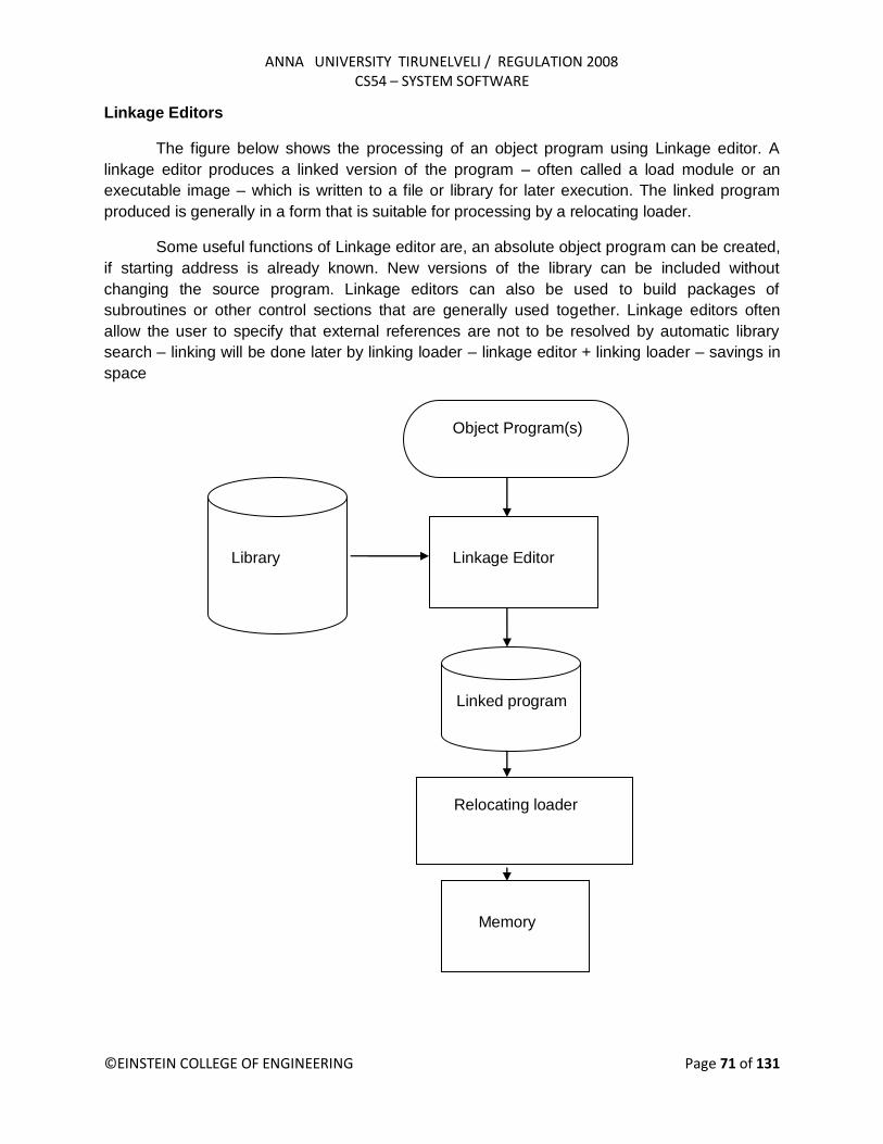
ANNA UNIVERSITY TIRUNELVELI / REGULATION 2008 CS54 – SYSTEM SOFTWARE
©EINSTEIN COLLEGE OF ENGINEERING Page 71 of 131
Linkage Editors
The figure below shows the processing of an object program using Linkage editor. A
linkage editor produces a linked version of the program – often called a load module or an
executable image – which is written to a file or library for later execution. The linked program
produced is generally in a form that is suitable for processing by a relocating loader.
Some useful functions of Linkage editor are, an absolute object program can be created,
if starting address is already known. New versions of the library can be included without
changing the source program. Linkage editors can also be used to build packages of
subroutines or other control sections that are generally used together. Linkage editors often
allow the user to specify that external references are not to be resolved by automatic library
search – linking will be done later by linking loader – linkage editor + linking loader – savings in
space
Library
Object Program(s)
Linkage Editor
Linked program
Memory
Relocating loader

ANNA UNIVERSITY TIRUNELVELI / REGULATION 2008 CS54 – SYSTEM SOFTWARE
©EINSTEIN COLLEGE OF ENGINEERING Page 72 of 131
Dynamic Linking
The scheme that postpones the linking functions until execution. A subroutine is loaded
and linked to the rest of the program when it is first called – usually called dynamic linking,
dynamic loading or load on call. The advantages of dynamic linking are, it allow several
executing programs to share one copy of a subroutine or library. In an object oriented system,
dynamic linking makes it possible for one object to be shared by several programs. Dynamic
linking provides the ability to load the routines only when (and if) they are needed. The actual
loading and linking can be accomplished using operating system service request.
Bootstrap Loaders
If the question, how is the loader itself loaded into the memory ? is asked, then the
answer is, when computer is started – with no program in memory, a program present in ROM (
absolute address) can be made executed – may be OS itself or A Bootstrap loader, which in
turn loads OS and prepares it for execution. The first record ( or records) is generally referred to
as a bootstrap loader – makes the OS to be loaded. Such a loader is added to the beginning of
all object programs that are to be loaded into an empty and idle system.
Implementation Examples
This section contains brief description of loaders and linkers for actual computers. They
are, MS-DOS Linker - Pentium architecture, SunOS Linkers - SPARC architecture, and, Cray
MPP Linkers – T3E architecture.
MS-DOS Linker
This explains some of the features of Microsoft MS-DOS linker, which is a linker for
Pentium and other x86 systems. Most MS-DOS compilers and assemblers (MASM) produce
object modules, and they are stored in .OBJ files. MS-DOS LINK is a linkage editor that
combines one or more object modules to produce a complete executable program - .EXE file;
this file is later executed for results.
The following table illustrates the typical MS-DOS object module
Record Types Description
THEADR Translator Header
TYPDEF,PUBDEF, EXTDEF External symbols and references
LNAMES, SEGDEF, GRPDEF Segment definition and grouping
LEDATA, LIDATA Translated instructions and data
FIXUPP Relocation and linking information
MODEND End of object module

ANNA UNIVERSITY TIRUNELVELI / REGULATION 2008 CS54 – SYSTEM SOFTWARE
©EINSTEIN COLLEGE OF ENGINEERING Page 73 of 131
THEADR specifies the name of the object module. MODEND specifies the end of the
module. PUBDEF contains list of the external symbols (called public names). EXTDEF contains
list of external symbols referred in this module, but defined elsewhere. TYPDEF the data types
are defined here. SEGDEF describes segments in the object module ( includes name, length,
and alignment). GRPDEF includes how segments are combined into groups. LNAMES contains
all segment and class names. LEDATA contains translated instructions and data. LIDATA has
above in repeating pattern. Finally, FIXUPP is used to resolve external references.
SunOS Linkers
SunOS Linkers are developed for SPARC systems. SunOS provides two different linkers
– link-editor and run-time linker.
Link-editor is invoked in the process of assembling or compiling a program – produces a
single output module – one of the following types
A relocatable object module – suitable for further link-editing
A static executable – with all symbolic references bound and ready to run
A dynamic executable – in which some symbolic references may need to be bound at run time
A shared object – which provides services that can be, bound at run time to one ore more
dynamic executables
An object module contains one or more sections – representing instructions and data
area from the source program, relocation and linking information, external symbol table.
Run-time linker uses dynamic linking approach. Run-time linker binds dynamic
executables and shared objects at execution time. Performs relocation and linking operations to
prepare the program for execution.
Cray MPP Linker
Cray MPP (massively parallel processing) Linker is developed for Cray T3E systems. A
T3E system contains large number of parallel processing elements (PEs) – Each PE has local
memory and has access to remote memory (memory of other PEs). The processing is divided
among PEs - contains shared data and private data. The loaded program gets copy of the
executable code, its private data and its portion of the shared data. The MPP linker organizes
blocks containing executable code, private data and shared data. The linker then writes an
executable file that contains the relocated and linked blocks. The executable file also specifies
the number of PEs required and other control information. The linker can create an executable
file that is targeted for a fixed number of PEs, or one that allows the partition size to be chosen
at run time. Latter type is called plastic executable.

ANNA UNIVERSITY TIRUNELVELI / REGULATION 2008 CS54 – SYSTEM SOFTWARE
©EINSTEIN COLLEGE OF ENGINEERING Page 74 of 131
UNIT IV - MACRO PROCESSORS
A Macro represents a commonly used group of statements in the source programming
language.
A macro instruction (macro) is a notational convenience for the programmer o It allows the programmer to write shorthand version of a program (module
programming)
The macro processor replaces each macro instruction with the corresponding group of source language statements (expanding)
o Normally, it performs no analysis of the text it handles. o It does not concern the meaning of the involved statements during macro
expansion.
The design of a macro processor generally is machine independent!
Two new assembler directives are used in macro definition o MACRO: identify the beginning of a macro definition o MEND: identify the end of a macro definition
Prototype for the macro o Each parameter begins with „&‟
name MACRO parameters :
body
:
MEND
o Body: the statements that will be generated as the expansion of the macro.
Basic Macro Processor Functions:
Macro Definition and Expansion
Macro Processor Algorithms and Data structures Macro Definition and Expansion:
The figure shows the MACRO expansion. The left block shows the MACRO definition
and the right block shows the expanded macro replacing the MACRO call with its block of
executable instruction.
M1 is a macro with two parameters D1 and D2. The MACRO stores the contents of
register A in D1 and the contents of register B in D2. Later M1 is invoked with the parameters
DATA1 and DATA2, Second time with DATA4 and DATA3. Every call of MACRO is expended
with the executable statements.

ANNA UNIVERSITY TIRUNELVELI / REGULATION 2008 CS54 – SYSTEM SOFTWARE
©EINSTEIN COLLEGE OF ENGINEERING Page 75 of 131
Fig 4.1
The statement M1 DATA1, DATA2 is a macro invocation statements that gives the name of the
macro instruction being invoked and the arguments (M1 and M2) to be used in expanding. A
macro invocation is referred as a Macro Call or Invocation.
Macro Expansion:
The program with macros is supplied to the macro processor. Each macro invocation
statement will be expanded into the statement s that form the body of the macro, with the
arguments from the macro invocation substituted for the parameters in the macro prototype.
During the expansion, the macro definition statements are deleted since they are no longer
needed.
The arguments and the parameters are associated with one another according to their
positions. The first argument in the macro matches with the first parameter in the macro
prototype and so on.
After macro processing the expanded file can become the input for the Assembler. The
Macro Invocation statement is considered as comments and the statement generated from
expansion is treated exactly as though they had been written directly by the programmer.
The difference between Macros and Subroutines is that the statement s from the body of
the Macro is expanded the number of times the macro invocation is encountered, whereas the
statement of the subroutine appears only once no matter how many times the subroutine is
called. Macro instructions will be written so that the body of the macro contains no labels.
Problem of the label in the body of macro: o If the same macro is expanded multiple times at different places in the program
… o There will be duplicate labels, which will be treated as errors by the assembler.
Solutions: o Do not use labels in the body of macro. o Explicitly use PC-relative addressing instead.
Ex, in RDBUFF and WRBUFF macros,

ANNA UNIVERSITY TIRUNELVELI / REGULATION 2008 CS54 – SYSTEM SOFTWARE
©EINSTEIN COLLEGE OF ENGINEERING Page 76 of 131
o JEQ *+11 o JLT *-14
It is inconvenient and error-prone.
The following program shows the concept of Macro Invocation and Macro Expansion.

ANNA UNIVERSITY TIRUNELVELI / REGULATION 2008 CS54 – SYSTEM SOFTWARE
©EINSTEIN COLLEGE OF ENGINEERING Page 77 of 131
Fig 4.2
Macro Processor Algorithm and Data Structure:
Design can be done as two-pass or a one-pass macro. In case of two-pass assembler.
Two-pass macro processor
You may design a two-pass macro processor o Pass 1:
Process all macro definitions o Pass 2:
Expand all macro invocation statements
However, one-pass may be enough o Because all macros would have to be defined during the first pass before any
macro invocations were expanded. The definition of a macro must appear before any statements that invoke
that macro.
Moreover, the body of one macro can contain definitions of the other macro
Consider the example of a Macro defining another Macro.
In the example below, the body of the first Macro (MACROS) contains statement that define RDBUFF, WRBUFF and other macro instructions for SIC machine.
The body of the second Macro (MACROX) defines the se same macros for SIC/XE machine.
A proper invocation would make the same program to perform macro invocation to run on either SIC or SIC/XEmachine.

ANNA UNIVERSITY TIRUNELVELI / REGULATION 2008 CS54 – SYSTEM SOFTWARE
©EINSTEIN COLLEGE OF ENGINEERING Page 78 of 131
MACROS for SIC machine
Fig 4.3(a)
MACROX for SIC/XE Machine
Fig 4.3(b)
A program that is to be run on SIC system could invoke MACROS whereas a program to be run on SIC/XE can invoke MACROX.
However, defining MACROS or MACROX does not define RDBUFF and WRBUFF.
These definitions are processed only when an invocation of MACROS or MACROX is expanded.

ANNA UNIVERSITY TIRUNELVELI / REGULATION 2008 CS54 – SYSTEM SOFTWARE
©EINSTEIN COLLEGE OF ENGINEERING Page 79 of 131
One-Pass Macro Processor:
A one-pass macro processor that alternate between macro definition and macro expansion in a recursive way is able to handle recursive macro definition.
Restriction o The definition of a macro must appear in the source program before any
statements that invoke that macro. o This restriction does not create any real inconvenience.
The design considered is for one-pass assembler. The data structures required are:
DEFTAB (Definition Table) o Stores the macro definition including macro prototype and
macro body
o Comment lines are omitted. o References to the macro instruction parameters are converted to a positional
notation for efficiency in substituting arguments.
NAMTAB (Name Table) o Stores macro names o Serves as an index to DEFTAB
Pointers to the beginning and the end of the macro definition (DEFTAB)
ARGTAB (Argument Table) o Stores the arguments according to their positions in the argument list. o As the macro is expanded the arguments from the Argument table are
substituted for the corresponding parameters in the macro body. o The figure below shows the different data structures described and their
relationship.
Fig 4.4

ANNA UNIVERSITY TIRUNELVELI / REGULATION 2008 CS54 – SYSTEM SOFTWARE
©EINSTEIN COLLEGE OF ENGINEERING Page 80 of 131
The above figure shows the portion of the contents of the table during the processing of the
program in page no. 3. In fig 4.4(a) definition of RDBUFF is stored in DEFTAB, with an entry in
NAMTAB having the pointers to the beginning and the end of the definition. The arguments
referred by the instructions are denoted by the their positional notations. For example,
TD =X‟?1‟
The above instruction is to test the availability of the device whose number is given by the
parameter &INDEV. In the instruction this is replaced by its positional value? 1.
Figure 4.4(b) shows the ARTAB as it would appear during expansion of the RDBUFF statement
as given below:
CLOOP RDBUFF F1, BUFFER, LENGTH
For the invocation of the macro RDBUFF, the first parameter is F1 (input device code),
second is BUFFER (indicating the address where the characters read are stored), and the third
is LENGTH (which indicates total length of the record to be read). When the ?n notation is
encountered in a line fro DEFTAB, a simple indexing operation supplies the proper argument
from ARGTAB.
The algorithm of the Macro processor is given below. This has the procedure DEFINE
to make the entry of macro name in the NAMTAB, Macro Prototype in DEFTAB. EXPAND is
called to set up the argument values in ARGTAB and expand a Macro Invocation statement.
Procedure GETLINE is called to get the next line to be processed either from the DEFTAB or
from the file itself.
When a macro definition is encountered it is entered in the DEFTAB. The normal
approach is to continue entering till MEND is encountered. If there is a program having a Macro
defined within another Macro. While defining in the DEFTAB the very first MEND is taken as the
end of the Macro definition. This does not complete the definition as there is another outer
Macro which completes the difintion of Macro as a whole. Therefore the DEFINE procedure
keeps a counter variable LEVEL. Every time a Macro directive is encountered this counter is
incremented by 1. The moment the innermost Macro ends indicated by the directive MEND it
starts decreasing the value of the counter variable by one. The last MEND should make the
counter value set to zero. So when LEVEL becomes zero, the MEND corresponds to the
original MACRO directive.
Most macro processors allow thr definitions of the commonly used instructions to appear
in a standard system library, rather than in the source program. This makes the use of macros
convenient; definitions are retrieved from the library as they are needed during macro
processing.

ANNA UNIVERSITY TIRUNELVELI / REGULATION 2008 CS54 – SYSTEM SOFTWARE
©EINSTEIN COLLEGE OF ENGINEERING Page 81 of 131
Fig 4.5
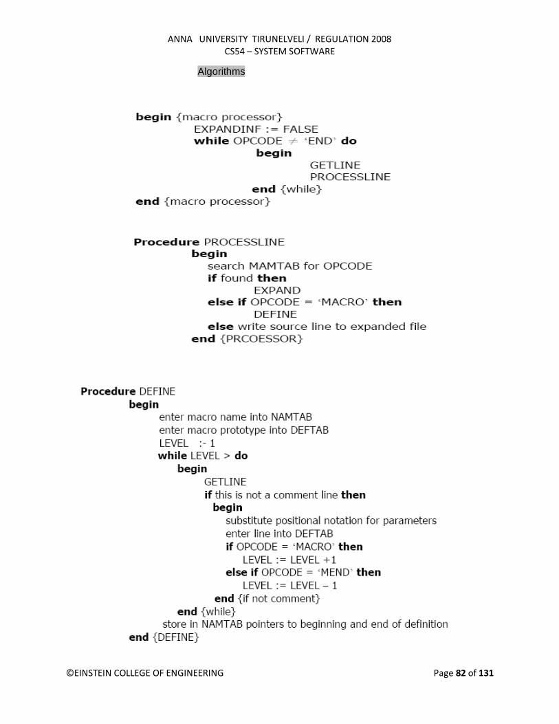
ANNA UNIVERSITY TIRUNELVELI / REGULATION 2008 CS54 – SYSTEM SOFTWARE
©EINSTEIN COLLEGE OF ENGINEERING Page 82 of 131
Algorithms

ANNA UNIVERSITY TIRUNELVELI / REGULATION 2008 CS54 – SYSTEM SOFTWARE
©EINSTEIN COLLEGE OF ENGINEERING Page 83 of 131
Fig 4.6
Comparison of Macro Processor Design
One-pass algorithm
o Every macro must be defined before it is called o One-pass processor can alternate between macro definition and macro
expansion o Nested macro definitions are allowed but nested calls are not allowed.
Two-pass algorithm
o Pass1: Recognize macro definitions o Pass2: Recognize macro calls o Nested macro definitions are not allowed

ANNA UNIVERSITY TIRUNELVELI / REGULATION 2008 CS54 – SYSTEM SOFTWARE
©EINSTEIN COLLEGE OF ENGINEERING Page 84 of 131
Machine-independent Macro-Processor Features.
The design of macro processor doesn‟t depend on the architecture of the machine. We
will be studying some extended feature for this macro processor. These features are:
Concatenation of Macro Parameters
Generation of unique labels
Conditional Macro Expansion
Keyword Macro Parameters
Concatenation of unique labels:
Most macro processor allows parameters to be concatenated with other character
strings. Suppose that a program contains a series of variables named by the symbols XA1,
XA2, XA3,…, another series of variables named XB1, XB2, XB3,…, etc. If similar processing is
to be performed on each series of labels, the programmer might put this as a macro instruction.
The parameter to such a macro instruction could specify the series of variables to be operated
on (A, B, etc.). The macro processor would use this parameter to construct the symbols
required in the macro expansion (XA1, Xb1, etc.).
Suppose that the parameter to such a macro instruction is named &ID. The body of the
macro definition might contain a statement like
LDA X&ID1
Fig 4.7
& is the starting character of the macro instruction; but the end of the parameter is not marked.
So in the case of &ID1, the macro processor could deduce the meaning that was intended. If the
macro definition contains contain &ID and &ID1 as parameters, the situation would be
unavoidably ambiguous.
Most of the macro processors deal with this problem by providing a special
concatenation operator. In the SIC macro language, this operator is the character . Thus the
statement LDA X&ID1 can be written as
LDA X&ID

ANNA UNIVERSITY TIRUNELVELI / REGULATION 2008 CS54 – SYSTEM SOFTWARE
©EINSTEIN COLLEGE OF ENGINEERING Page 85 of 131
Fig 4.8
The above figure shows a macro definition that uses the concatenation operator as
previously described. The statement SUM A and SUM BETA shows the invocation statements
and the corresponding macro expansion.
Generation of Unique Labels
As discussed it is not possible to use labels for the instructions in the macro definition,
since every expansion of macro would include the label repeatedly which is not allowed by the
assembler. This in turn forces us to use relative addressing in the jump instructions. Instead we
can use the technique of generating unique labels for every macro invocation and expansion.
During macro expansion each $ will be replaced with $XX, where xx is a two-character
alphanumeric counter of the number of macro instructions expansion.

ANNA UNIVERSITY TIRUNELVELI / REGULATION 2008 CS54 – SYSTEM SOFTWARE
©EINSTEIN COLLEGE OF ENGINEERING Page 86 of 131
For example,
XX = AA, AB, AC…
This allows 1296 macro expansions in a single program.
The following program shows the macro definition with labels to the instruction.
The following figure shows the macro invocation and expansion first time.

ANNA UNIVERSITY TIRUNELVELI / REGULATION 2008 CS54 – SYSTEM SOFTWARE
©EINSTEIN COLLEGE OF ENGINEERING Page 87 of 131
If the macro is invoked second time the labels may be expanded as $ABLOOP
$ABEXIT.
Conditional Macro Expansion
There are applications of macro processors that are not related to assemblers or
assembler programming. Conditional assembly depends on parameters provides
MACRO &COND
……..
IF (&COND NE „‟)
part I
ELSE
part II
ENDIF
………
ENDM

ANNA UNIVERSITY TIRUNELVELI / REGULATION 2008 CS54 – SYSTEM SOFTWARE
©EINSTEIN COLLEGE OF ENGINEERING Page 88 of 131
Part I is expanded if condition part is true, otherwise part II is expanded. Compare operators:
NE, EQ, LE, GT.
Macro-Time Variables:
Macro-time variables (often called as SET Symbol) can be used to store working values
during the macro expansion. Any symbol that begins with symbol & and not a macro instruction
parameter is considered as macro-time variable. All such variables are initialized to zero.
Fig 4.9(a)
Figure 4.5(a) gives the definition of the macro RDBUFF with the parameters &INDEV,
&BUFADR, &RECLTH, &EOR, &MAXLTH. According to the above program if &EOR has any
value, then &EORCK is set to 1 by using the directive SET, otherwise it retains its default value
0.

ANNA UNIVERSITY TIRUNELVELI / REGULATION 2008 CS54 – SYSTEM SOFTWARE
©EINSTEIN COLLEGE OF ENGINEERING Page 89 of 131
Fig 4.9(b) Use of Macro-Time Variable with EOF being NOT NULL
Fig 4.9(c) Use of Macro-Time conditional statement with EOF being NULL

ANNA UNIVERSITY TIRUNELVELI / REGULATION 2008 CS54 – SYSTEM SOFTWARE
©EINSTEIN COLLEGE OF ENGINEERING Page 90 of 131
Fig 4.9(d) Use of Time-variable with EOF NOT NULL and MAXLENGTH being NULL
The above programs show the expansion of Macro invocation statements with different values
for the time variables. In figure 4.9(b) the &EOF value is NULL. When the macro invocation is
done, IF statement is executed, if it is true EORCK is set to 1, otherwise normal execution of the
other part of the program is continued.
The macro processor must maintain a symbol table that contains the value of all macro-time
variables used. Entries in this table are modified when SET statements are processed. The
table is used to look up the current value of the macro-time variable whenever it is required.
When an IF statement is encountered during the expansion of a macro, the specified Boolean
expression is evaluated.
If the value of this expression TRUE,
The macro processor continues to process lines from the DEFTAB until it encounters the ELSE or ENDIF statement.
If an ELSE is found, macro processor skips lines in DEFTAB until the next ENDIF.
Once it reaches ENDIF, it resumes expanding the macro in the usual way. If the value of the expression is FALSE,
The macro processor skips ahead in DEFTAB until it encounters next ELSE or ENDIF statement.
The macro processor then resumes normal macro expansion. The macro-time IF-ELSE-ENDIF structure provides a mechanism for either generating(once) or
skipping selected statements in the macro body. There is another construct WHILE statement
which specifies that the following line until the next ENDW statement, are to be generated
repeatedly as long as a particular condition is true. The testing of this condition, and the looping

ANNA UNIVERSITY TIRUNELVELI / REGULATION 2008 CS54 – SYSTEM SOFTWARE
©EINSTEIN COLLEGE OF ENGINEERING Page 91 of 131
are done during the macro is under expansion. The example shown below shows the usage of
Macro-Time Looping statement.
WHILE-ENDW structure
When an WHILE statement is encountered during the expansion of a macro, the specified Boolean expression is evaluated.
TRUE o The macro processor continues to process lines from DEFTAB until it encounters
the next ENDW statement. o When ENDW is encountered, the macro processor returns to the preceding
WHILE, re-evaluates the Boolean expression, and takes action based on the new value.
FALSE o The macro processor skips ahead in DEFTAB until it finds the next ENDW
statement and then resumes normal macro expansion.

ANNA UNIVERSITY TIRUNELVELI / REGULATION 2008 CS54 – SYSTEM SOFTWARE
©EINSTEIN COLLEGE OF ENGINEERING Page 92 of 131
Keyword Macro Parameters
All the macro instruction definitions used positional parameters. Parameters and
arguments are matched according to their positions in the macro prototype and the macro
invocation statement. The programmer needs to be careful while specifying the arguments. If an
argument is to be omitted the macro invocation statement must contain a null argument
mentioned with two commas.
Positional parameters are suitable for the macro invocation. But if the macro invocation
has large number of parameters, and if only few of the values need to be used in a typical
invocation, a different type of parameter specification is required (for example, in many cases
most of the parameters may have default values, and the invocation may mention only the
changes from the default values).
Ex: XXX MACRO &P1, &P2, …., &P20, ….
XXX A1, A2,,,,,,,,,,…,,A20,…..
Null arguments
Keyword parameters
Each argument value is written with a keyword that names the corresponding parameter.
Arguments may appear in any order.
Null arguments no longer need to be used.
Ex: XXX P1=A1, P2=A2, P20=A20.
It is easier to read and much less error-prone than the positional method.

ANNA UNIVERSITY TIRUNELVELI / REGULATION 2008 CS54 – SYSTEM SOFTWARE
©EINSTEIN COLLEGE OF ENGINEERING Page 93 of 131

ANNA UNIVERSITY TIRUNELVELI / REGULATION 2008 CS54 – SYSTEM SOFTWARE
©EINSTEIN COLLEGE OF ENGINEERING Page 94 of 131
Fig 4.10 Example showing the usage of Keyword Parameter
Macro Processor Design Options Recursive Macro Expansion
We have seen an example of the definition of one macro instruction by another. But we have
not dealt with the invocation of one macro by another. The following example shows the
invocation of one macro by another macro.
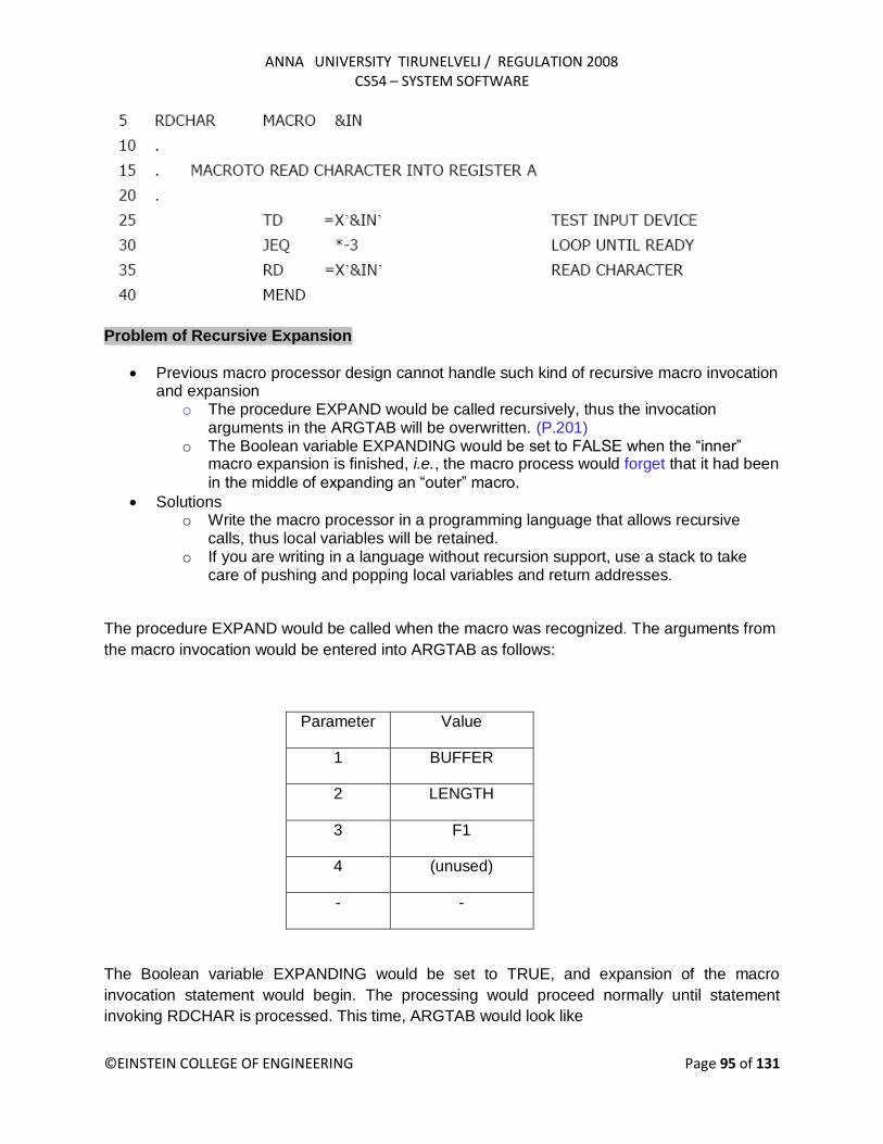
ANNA UNIVERSITY TIRUNELVELI / REGULATION 2008 CS54 – SYSTEM SOFTWARE
©EINSTEIN COLLEGE OF ENGINEERING Page 95 of 131
Problem of Recursive Expansion
Previous macro processor design cannot handle such kind of recursive macro invocation and expansion
o The procedure EXPAND would be called recursively, thus the invocation arguments in the ARGTAB will be overwritten. (P.201)
o The Boolean variable EXPANDING would be set to FALSE when the “inner” macro expansion is finished, i.e., the macro process would forget that it had been
in the middle of expanding an “outer” macro.
Solutions o Write the macro processor in a programming language that allows recursive
calls, thus local variables will be retained. o If you are writing in a language without recursion support, use a stack to take
care of pushing and popping local variables and return addresses.
The procedure EXPAND would be called when the macro was recognized. The arguments from
the macro invocation would be entered into ARGTAB as follows:
Parameter Value
1 BUFFER
2 LENGTH
3 F1
4 (unused)
- -
The Boolean variable EXPANDING would be set to TRUE, and expansion of the macro
invocation statement would begin. The processing would proceed normally until statement
invoking RDCHAR is processed. This time, ARGTAB would look like

ANNA UNIVERSITY TIRUNELVELI / REGULATION 2008 CS54 – SYSTEM SOFTWARE
©EINSTEIN COLLEGE OF ENGINEERING Page 96 of 131
Parameter Value
1 F1
2 (Unused)
-- --
At the expansion, when the end of RDCHAR is recognized, EXPANDING would be set to
FALSE. Thus the macro processor would „forget‟ that it had been in the middle of expanding a
macro when it encountered the RDCHAR statement. In addition, the arguments from the original
macro invocation (RDBUFF) would be lost because the value in ARGTAB was overwritten with
the arguments from the invocation of RDCHAR.
General-Purpose Macro Processors
Macro processors that do not dependent on any particular programming language, but can be used with a variety of different languages
Pros o Programmers do not need to learn many macro languages. o Although its development costs are somewhat greater than those for a language
specific macro processor, this expense does not need to be repeated for each language, thus save substantial overall cost.
Cons
o Large number of details must be dealt with in a real programming language Situations in which normal macro parameter substitution should not
occur, e.g., comments. Facilities for grouping together terms, expressions, or statements Tokens, e.g., identifiers, constants, operators, keywords Syntax had better be consistent with the source programming language
Macro Processing within Language Translators
The macro processors we discussed are called “Preprocessors”. o Process macro definitions o Expand macro invocations o Produce an expanded version of the source program, which is then used as input to
an assembler or compiler
You may also combine the macro processing functions with the language translator: o Line-by-line macro processor o Integrated macro processor

ANNA UNIVERSITY TIRUNELVELI / REGULATION 2008 CS54 – SYSTEM SOFTWARE
©EINSTEIN COLLEGE OF ENGINEERING Page 97 of 131
Line-by-Line Macro Processor
o Used as a sort of input routine for the assembler or compiler o Read source program o Process macro definitions and expand macro invocations o Pass output lines to the assembler or compiler
Benefits o Avoid making an extra pass over the source program. o Data structures required by the macro processor and the language translator can be
combined (e.g., OPTAB and NAMTAB) o Utility subroutines can be used by both macro processor and the language translator.
Scanning input lines Searching tables Data format conversion
o It is easier to give diagnostic messages related to the source statements
Integrated Macro Processor
An integrated macro processor can potentially make use of any information about the source program that is extracted by the language translator.
o Ex (blanks are not significant in FORTRAN) DO 100 I = 1,20
a DO statement DO 100 I = 1
An assignment statement
DO100I: variable (blanks are not significant in FORTRAN)
An integrated macro processor can support macro instructions that depend upon the context in which they occur.

ANNA UNIVERSITY TIRUNELVELI / REGULATION 2008 CS54 – SYSTEM SOFTWARE
©EINSTEIN COLLEGE OF ENGINEERING Page 98 of 131
UNIT V - TEXT- EDITORS
These are the primary interface to the computer for all types of “Knowledge workers” as they
compose, organize, study and manipulate computer-based information.
OVERVIEW OF THE EDITING PROCESS.
An interactive editor is a computer program that allows a user to create and revise a
target document.The term document includes objects such as computer programs, texts,
equations, tables, diagrams, line art and photographs-anything that one might find on a
printed page. Text editor is one in which the primary elements being edited are character
strings of the target text.
The document editing process is an interactive user-computer dialogue designed to accomplish
four tasks:
1) Select the part of the target document to be viewed and manipulated 2) Determine how to format this view on-line and how to display it. 3) Specify and execute operations that modify the target document. 4) Update the view appropriately.
Traveling – Selection of the part of the document to be viewed and edited. It involves first
traveling through the document to locate the area of interest such as “next screenful”,
”bottom”,and “find pattern”. Traveling specifies where the area of interest is;
Filtering - The selection of what is to be viewed and manipulated is controlled by filtering.
Filtering extracts the relevant subset of the target document at the point of interest such as next
screenful of text or next statement.
Formatting: Formatting determines how the result of filtering will be seen as a visible
representation (the view) on a display screen or other device.
Editing: In the actual editing phase, the target document is created or altered with a set of
operations such as insert, delete, replace, move or copy.

ANNA UNIVERSITY TIRUNELVELI / REGULATION 2008 CS54 – SYSTEM SOFTWARE
©EINSTEIN COLLEGE OF ENGINEERING Page 99 of 131
Manuscript oriented editors operate on elements such as single characters, words, lines,
sentences and paragraphs;
Program-oriented editors operates on elements such as identifiers, keywords and statements
THE USER-INTERFACE OF AN EDITOR.
The user of an interactive editor is presented with a conceptual model of the editing
system. The model is an abstract framework on which the editor and the world on which the
operations are based.
The line editors simulated the world of the keypunch they allowed operations on
numbered sequence of 80-character card image lines.
The Screen-editors define a world in which a document is represented as a quarter-
plane of text lines, unbounded both down and to the right. The user sees, through a cutout, only
a rectangular subset of this plane on a multi line display terminal. The cutout can be moved left
or right, and up or down, to display other portions of the document.
The user interface is also concerned with the input devices, the output devices, and
the interaction language of the system.
INPUT DEVICES: The input devices are used to enter elements of text being edited, to enter
commands, and to designate editable elements.
Input devices are categorized as:
1) Text devices
2) Button devices
3) Locator devices
1) Text or string devices are typically typewriter like keyboards on which user presses and
release keys, sending unique code for each key. Virtually all computer key boards are of the
QWERTY type.

ANNA UNIVERSITY TIRUNELVELI / REGULATION 2008 CS54 – SYSTEM SOFTWARE
©EINSTEIN COLLEGE OF ENGINEERING Page 100 of 131
2) Button or Choice devices generate an interrupt or set a system flag, usually causing an
invocation of an associated application program. Also special function keys are also available
on the key board. Alternatively, buttons can be simulated in software by displaying text strings
or symbols on the screen. The user chooses a string or symbol instead of pressing a button.
3) Locator devices: They are two-dimensional analog-to-digital converters that position a
cursor symbol on the screen by observing the user‟s movement of the device. The most
common such devices are the mouse and the tablet.
The Data Tablet is a flat, rectangular, electromagnetically sensitive panel. Either the
ballpoint pen like stylus or a puck, a small device similar to a mouse is moved over the surface.
The tablet returns to a system program the co-ordinates of the position on the data tablet at
which the stylus or puck is currently located. The program can then map these data-tablet
coordinates to screen coordinates and move the cursor to the corresponding screen position.
Text devices with arrow (Cursor) keys can be used to simulate locator devices. Each
of these keys shows an arrow that point up, down, left or right. Pressing an arrow key typically
generates an appropriate character sequence; the program interprets this sequence and moves
the cursor in the direction of the arrow on the key pressed.
VOICE-INPUT DEVICES: which translate spoken words to their textual equivalents, may prove
to be the text input devices of the future. Voice recognizers are currently available for command
input on some systems.
OUTPUT DEVICES
The output devices let the user view the elements being edited and the result of the
editing operations.
The first output devices were teletypewriters and other character-printing terminals that
generated output on paper.
Next “glass teletypes” based on Cathode Ray Tube (CRT) technology which uses CRT screen essentially to simulate the hard-copy teletypewriter.
Today‟s advanced CRT terminals use hardware assistance for such features as
moving the cursor, inserting and deleting characters and lines, and scrolling lines and pages.
The modern professional workstations are based on personal computers with high
resolution displays; support multiple proportionally spaced character fonts to produce realistic facsimiles of hard copy documents.
ANNA UNIVERSITY TIRUNELVELI / REGULATION 2008 CS54 – SYSTEM SOFTWARE
©EINSTEIN COLLEGE OF ENGINEERING Page 101 of 131
INTERACTION LANGUAGE:
The interaction language of the text editor is generally one of several common
types.
The typing oriented or text command-oriented method
It is the oldest of the major editing interfaces. The user communicates with the editor by
typing text strings both for command names and for operands. These strings are sent to the
editor and are usually echoed to the output device.
Typed specification often requires the user to remember the exact form of all commands,
or at least their abbreviations. If the command language is complex, the user must continually
refer to a manual or an on-line Help function. The typing required can be time consuming for in-
experienced users.
Function key interfaces:
Each command is associated with marked key on the key board. This eliminates much
typing. E.g.: Insert key, Shift key, Control key
Disadvantages:
Have too many unique keys
Multiple key stroke commands
Menu oriented interface
A menu is a multiple choice set of text strings or icons which are graphical symbols that
represent objects or operations. The user can perform actions by selecting items for the menus.
The editor prompts the user with a menu. One problem with menu oriented system can arise
when there are many possible actions and several choices are required to complete an action.
The display area of the menu is rather limited

ANNA UNIVERSITY TIRUNELVELI / REGULATION 2008 CS54 – SYSTEM SOFTWARE
©EINSTEIN COLLEGE OF ENGINEERING Page 102 of 131
EDITOR STRUCTURE
Most Text editors have a structure similar to that shown above.
The command Language Processor
It accepts input from the user‟s input devices, and analyzes the tokens and
syntactic structure of the commands. It functions much like the lexical and syntactic phases of a
compiler. The command language processor may invoke the semantic routines directly. In a text
editor, these semantic routines perform functions such as editing and viewing.
The semantic routines involve traveling, editing, viewing and display functions.
Editing operations are always specified by the user and display operations are specified
implicitly by the other three categories of operations. Traveling and viewing operations may be
invoked either explicitly by the user or implicitly by the editing operations.
Editing
component
Traveling
component
Viewing
component
Command
language
processor
Editing
buffer Editing
filter
Viewing
filter Viewing
buffer
Main
memory
File
system
Display
component
Output
devices
input
Paging
Routines
Control
Data

ANNA UNIVERSITY TIRUNELVELI / REGULATION 2008 CS54 – SYSTEM SOFTWARE
©EINSTEIN COLLEGE OF ENGINEERING Page 103 of 131
Editing Component
In editing a document, the start of the area to be edited is determined by the current
editing pointer maintained by the editing component, which is the collection of modules dealing
with editing tasks. The current editing pointer can be set or reset explicitly by the user using
travelling commands, such as next paragraph and next screen, or implicitly as a side effect of
the previous editing operation such as delete paragraph.
Traveling Component
The traveling component of the editor actually performs the setting of the current editing
and viewing pointers, and thus determines the point at which the viewing and /or editing filtering
begins.
Viewing Component
The start of the area to be viewed is determined by the current viewing pointer. This
pointer is maintained by the viewing component of the editor, which is a collection of modules
responsible for determining the next view. The current viewing pointer can be set or reset
explicitly by the user or implicitly by system as a result of previous editing operation.
The viewing component formulates an ideal view, often expressed in a device
independent intermediate representation. This view may be a very simple one consisting of a
window‟s worth of text arranged so that lines are not broken in the middle of the words.
Display Component
It takes the idealized view from the viewing component and maps it to a physical output
device in the most efficient manner. The display component produces a display by mapping the
buffer to a rectangular subset of the screen, usually a window
Editing Filter
Filtering consists of the selection of contiguous characters beginning at the current point.
The editing filter filters the document to generate a new editing buffer based on the current
editing pointer as well as on the editing filter parameters
Editing Buffer
It contains the subset of the document filtered by the editing filter based on the editing
pointer and editing filter parameters

ANNA UNIVERSITY TIRUNELVELI / REGULATION 2008 CS54 – SYSTEM SOFTWARE
©EINSTEIN COLLEGE OF ENGINEERING Page 104 of 131
Viewing Filter
When the display needs to be updated, the viewing component invokes the viewing filter.
This component filters the document to generate a new viewing buffer based on the current
viewing pointer as well as on the viewing filter parameters.
Viewing Buffer
It contains the subset of the document filtered by the viewing filter based on the viewing
pointer and viewing filter parameters.
E.g. The user of a certain editor might travel to line 75,and after viewing it, decide to
change all occurrences of “ugly duckling” to “swan” in lines 1 through 50 of the file by using a
change command such as
[1,50] c/ugly duckling/swan/
As a part of the editing command there is implicit travel to the first line of the file. Lines 1
through 50 are then filtered from the document to become the editing buffer. Successive
substitutions take place in this editing buffer without corresponding updates of the view
In Line editors, the viewing buffer may contain the current line; in screen editors, this
buffer may contain rectangular cut out of the quarter-plane of text. This viewing buffer is then
passed to the display component of the editor, which produces a display by mapping the buffer
to a rectangular subset of the screen, usually called a window.
The editing and viewing buffers, while independent, can be related in many ways. In a
simplest case, they are identical: the user edits the material directly on the screen. On the other
hand, the editing and viewing buffers may be completely disjoint.

ANNA UNIVERSITY TIRUNELVELI / REGULATION 2008 CS54 – SYSTEM SOFTWARE
©EINSTEIN COLLEGE OF ENGINEERING Page 105 of 131
Windows typically cover the entire screen or rectangular portion of it. Mapping viewing
buffers to windows that cover only part of the screen is especially useful for editors on modern
graphics based workstations. Such systems can support multiple windows, simultaneously
showing different portions of the same file or portions of different file. This approach allows the
user to perform inter-file editing operations much more effectively than with a system only a
single window.
The mapping of the viewing buffer to a window is accomplished by two components of
the system.
(i) First, the viewing component formulates an ideal view often expressed in a device independent intermediate representation. This view may be a very
simple one consisting of a windows worth of text arranged so that lines are not broken in the middle of words. At the other extreme, the idealized view may be a facsimile of a page of fully formatted and typeset text with equations, tables and figures.
(ii) Second the display component takes these idealized views from the viewing component and maps it to a physical output device the most efficient manner possible.
The components of the editor deal with a user document on two levels:
(i) In main memory and
(ii) In the disk file system.
Loading an entire document into main memory may be infeasible. However if only part of
a document is loaded and if many user specified operations require a disk read by the editor to
locate the affected portions, editing might be unacceptably slow. In some systems this problem
is solved by the mapping the entire file into virtual memory and letting the operating system
perform efficient demand paging.
An alternative is to provide is the editor paging routines which read one or more logical
portions of a document into memory as needed. Such portions are often termed pages,
although there is usually no relationship between these pages and the hard copy document
pages or virtual memory pages. These pages remain resident in main memory until a user
operation requires that another portion of the document be loaded.
Editors function in three basic types of computing environment:
(i) Time-sharing environment (ii) Stand-alone environment and (iii) Distributed environment.
Each type of environment imposes some constraint on the design of an editor.
The Time –Sharing Environment
The time sharing editor must function swiftly within the context of the load on the
computer‟s processor, central memory and I/O devices.

ANNA UNIVERSITY TIRUNELVELI / REGULATION 2008 CS54 – SYSTEM SOFTWARE
©EINSTEIN COLLEGE OF ENGINEERING Page 106 of 131
The Stand alone Environment
The editor on a stand-alone system must have access to the functions that the time
sharing editors obtain from its host operating system. This may be provided in pare by a small
local operating system or they may be built into the editor itself if the stand alone system is
dedicated to editing.
Distributed Environment
The editor operating in a distributed resource sharing local network must, like a
standalone editor, run independently on each user‟s machine and must, like a time sharing
editor, content for shared resources such as files.
INTERACTIVE DEBUGGING SYSTEMS
An interactive debugging system provides programmers with facilities that
aid in testing and debugging of programs interactively.
DEBUGGING FUNCTIONS AND CAPABILITIES
Execution sequencing:
It is the observation and control of the flow of program execution. For example,
the program may be halted after a fixed number of instructions are executed.
Breakpoints – The programmer may define break points which cause execution
to be suspended, when a specified point in the program is reached. After execution is
suspended, the debugging command is used to analyze the progress of the program and to
diagnose errors detected. Execution of the program can then be removed.
Conditional Expressions – Programmers can define some conditional
expressions, evaluated during the debugging session, program execution is suspended,
when conditions are met, analysis is made, later execution is resumed
Gaits- Given a good graphical representation of program progress may even be
useful in running the program in various speeds called gaits.
A Debugging system should also provide functions such as tracing and traceback.
Tracing can be used to track the flow of execution logic and data modifications. The control
flow can be traced at different levels of detail – procedure, branch, individual instruction, and
so on…

ANNA UNIVERSITY TIRUNELVELI / REGULATION 2008 CS54 – SYSTEM SOFTWARE
©EINSTEIN COLLEGE OF ENGINEERING Page 107 of 131
Traceback can show the path by which the current statement in the program was reached. It
can also show which statements have modified a given variable or parameter. The
statements are displayed rather than as hexadecimal displacements.
Program-display Capabilities
It is also important for a debugging system to have good program display
capabilities. It must be possible to display the program being debugged, complete with
statement numbers.
Multilingual Capability
A debugging system should consider the language in which the program being
debugged is written. Most user environments and many applications systems involve the
use of different programming languages. A single debugging tool should be available to
multilingual situations.
Context Effects
The context being used has many different effects on the debugging interaction.
For example. The statements are different depending on the language
COBOL - MOVE 6.5 TO X
FORTRAN - X = 6.5
Likewise conditional statements should use the notation of the source language
COBOL - IF A NOT EQUAL TO B
FORTRAN - IF (A .NE. B)
Similar differences exist with respect to the form of statement labels, keywords and so on.
Display of source code
The language translator may provide the source code or source listing tagged in
some standard way so that the debugger has a uniform method of navigating about it.
Optimization:
It is also important that a debugging system be able to deal with optimized code.
Many optimizations involve the rearrangement of segments of code in the program.

ANNA UNIVERSITY TIRUNELVELI / REGULATION 2008 CS54 – SYSTEM SOFTWARE
©EINSTEIN COLLEGE OF ENGINEERING Page 108 of 131
For eg.
- invariant expressions can be removed from loop - separate loops can be combined into a single loop - redundant expression may be eliminated - elimination of unnecessary branch instructions
The debugging of optimized code requires a substantial amount of cooperation
from the optimizing compiler.
Relationship with Other Parts of the System
An interactive debugger must be related to other parts of the system in many
different ways.
Availability
Interactive debugger must appear to be a part of the run-time environment and
an integral part of the system. When an error is discovered, immediate debugging must be
possible because it may be difficult or impossible to reproduce the program failure in some
other environment or at some other times.
Consistency with security and integrity components
User need to be able to debug in a production environment. When an application
fails during a production run, work dependent on that application stops. Since the production
environment is often quite different from the test environment, many program failures cannot
be repeated outside the production environment.
Debugger must also exist in a way that is consistent with the security and
integrity components of the system. Use of debugger must be subjected to the normal
authorization mechanism and must leave the usual audit trails. Someone (unauthorized
user) must not access any data or code. It must not be possible to use the debuggers to
interface with any aspect of system integrity.
Coordination with existing and future systems
The debugger must co-ordinate its activities with those of existing and future
language compilers and interpreters.
It is assumed that debugging facilities in existing language will continue to exist
and be maintained. The requirement of cross-language debugger assumes that such a
facility would be installed as an alternative to the individual language debuggers.
USER- INTERFACE CRITERIA
The interactive debugging system should be user friendly. The facilities of debugging
system should be organized into few basic categories of functions which should closely reflect
common user tasks.

ANNA UNIVERSITY TIRUNELVELI / REGULATION 2008 CS54 – SYSTEM SOFTWARE
©EINSTEIN COLLEGE OF ENGINEERING Page 109 of 131
Full – screen displays and windowing systems
The user interaction should make use of full-screen display and windowing systems. The advantage of such interface is that the information can be should displayed and changed easily and quickly.
Menus:
With menus and full screen editors, the user has far less information to enter and remember
It should be possible to go directly to the menus without having to retrace an entire hierarchy.
When a full-screen terminal device is not available, user should have an equivalent action in a linear debugging language by providing commands.
Command language:
The command language should have a clear, logical, simple syntax. Parameters names should be consistent across set of commands
Parameters should automatically be checked for errors for type and range values. Defaults should be provided for parameters. Command language should minimize punctuations such as parenthesis, slashes, and
special characters. On Line HELP facility
Good interactive system should have an on-line HELP facility that should provide help for all options of menu
Help should be available from any state of the debugging system.

ANNA UNIVERSITY TIRUNELVELI / REGULATION 2008 CS54 – SYSTEM SOFTWARE
©EINSTEIN COLLEGE OF ENGINEERING Page 110 of 131
UNIT I - INTRODUCTION
1. Define system software.
It consists of variety of programs that supports the operation of the computer. This
software makes it possible for the user to focus on the other problems to be solved without needing
to know how the machine works internally.
Eg: operating system, assembler, loader.
2. Give some applications of operating system.
to make the computer easier to use
to manage the resources in computer
process management
data and memory management
to provide security to the user.
Operating system acts as an interface between the user and the system
Eg: windows, linux, unix, dos
3. Define compiler and interpreter.
Compiler is a set of program which converts the whole high level language program to
machine language program.
Interpreter is a set of programs which converts high level language program to machine
language program line by line.
4. Define loader.
Loader is a set of program that loads the machine language translated by the translator into
the main memory and makes it ready for execution.
5. What is the need of MAR register?
MAR (memory address register) is used to store the address of the memory from which the
data is to be read or to which the data is to be written.
6. Define indirect addressing

ANNA UNIVERSITY TIRUNELVELI / REGULATION 2008 CS54 – SYSTEM SOFTWARE
©EINSTEIN COLLEGE OF ENGINEERING Page 111 of 131
In the case of immediate addressing the operand field gives the memory location. The word from the
given address is fetched and it gives the address of the operand.
Eg:ADD R5, [600]
Here the second operand is given in indirect addressing mode. First the word in memory location 600
is fetched and which will give the address of the operand.
7. Define immediate addressing.
In this addressing mode the operand value is given directly. There is no need to refer
memory. The immediate addressing is indicated by the prefix „#‟.
Eg: ADD #5
In this instruction one operand is in accumulator and the second operand is an immediate value the
value 5 is directly added with the accumulator content and the result is stored in accumulator.
8. List out any two CISC and RISC machine.
CISC –Power PC, Cray T3E
RISC – VAX, Pentium Pro architecture
9. What is the name of A and L register in SIC machine and also specify its use.
A-accumulator
Used for arithmetic operation. i.e., in the case of arithmetic operations one operand is in the
accumulator, and other operand may be an immediate value, register operand or memory content.
The operation given in the instruction is performed and the result is stored in the accumulator
register.
L-linkage register
It is used to store the return address in the case of jump to subroutine (JSUB) instructions.
10. What are the instruction formats used in SIC/XE architecture? Give any one
format.
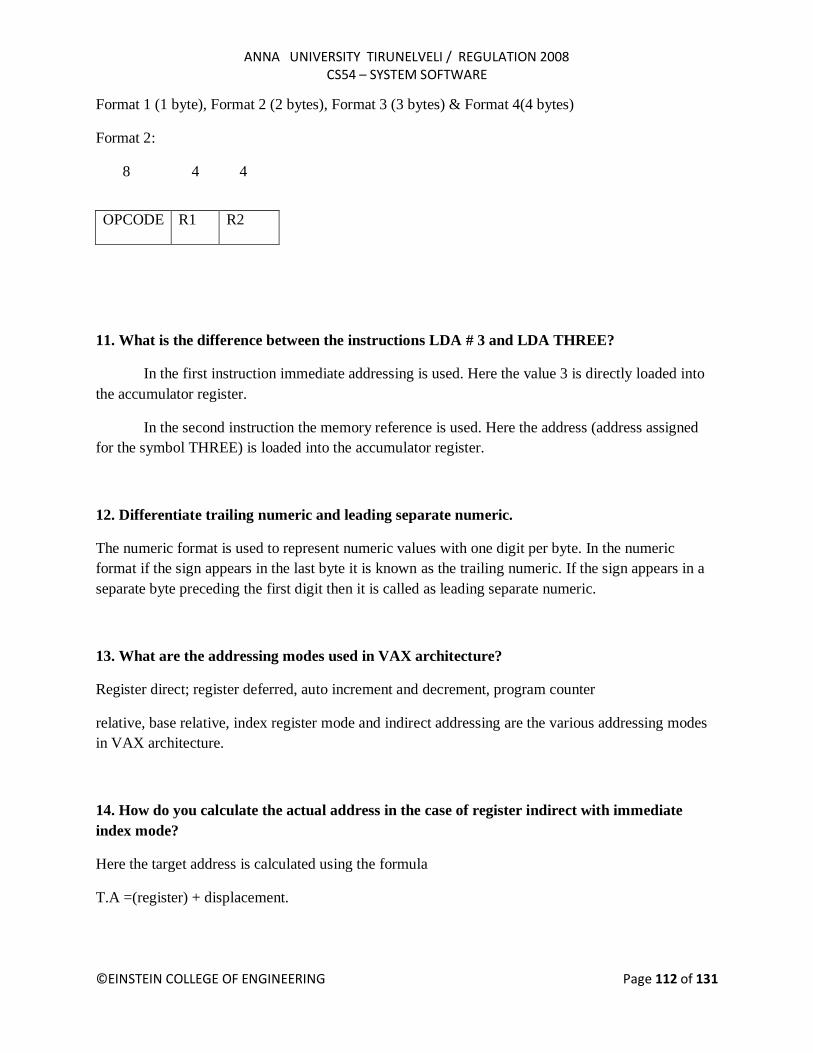
ANNA UNIVERSITY TIRUNELVELI / REGULATION 2008 CS54 – SYSTEM SOFTWARE
©EINSTEIN COLLEGE OF ENGINEERING Page 112 of 131
Format 1 (1 byte), Format 2 (2 bytes), Format 3 (3 bytes) & Format 4(4 bytes)
Format 2:
8 4 4
11. What is the difference between the instructions LDA # 3 and LDA THREE?
In the first instruction immediate addressing is used. Here the value 3 is directly loaded into
the accumulator register.
In the second instruction the memory reference is used. Here the address (address assigned
for the symbol THREE) is loaded into the accumulator register.
12. Differentiate trailing numeric and leading separate numeric.
The numeric format is used to represent numeric values with one digit per byte. In the numeric
format if the sign appears in the last byte it is known as the trailing numeric. If the sign appears in a
separate byte preceding the first digit then it is called as leading separate numeric.
13. What are the addressing modes used in VAX architecture?
Register direct; register deferred, auto increment and decrement, program counter
relative, base relative, index register mode and indirect addressing are the various addressing modes
in VAX architecture.
14. How do you calculate the actual address in the case of register indirect with immediate
index mode?
Here the target address is calculated using the formula
T.A =(register) + displacement.
OPCODE R1 R2
ANNA UNIVERSITY TIRUNELVELI / REGULATION 2008 CS54 – SYSTEM SOFTWARE
©EINSTEIN COLLEGE OF ENGINEERING Page 113 of 131
15. Write the sequence of instructions to perform the operation BETA = ALPHA + 1 using SIC
instructions.
LDA ALPHA
ADD ONE
STA BETA
…. ….
ALPHA RESW 1
BETA RESW 1
ONE RESW 1
16. Write the sequence of instructions to perform the operation BETA = ALPHA+5 using
SIC/XE instructions.
LDA ALPHA
ADD #1
STA BETA
…. ….
ALPHA RESW 1
BETA RESW 1
17. What is the use of TD instruction in SIC architecture?
The test device (TD) instruction tests whether the addressed device is ready to send or
receive a byte of data. The condition code is set to indicate the result of this test. Setting of < means
the device is ready to send or receive, and = means the device is not ready.
18. Give the instruction set of SIC / XE.
Load and store instruction
Arithmetic instruction
Register Move

ANNA UNIVERSITY TIRUNELVELI / REGULATION 2008 CS54 – SYSTEM SOFTWARE
©EINSTEIN COLLEGE OF ENGINEERING Page 114 of 131
Floating point arithmetic operations
Supervisor call instruction
Conditional jump
Subroutine linkages
19. Give the instruction set of SIC.
Load and store instruction
Arithmetic instruction
Conditional jump instruction
Subroutine linkages
20. What are the various data formats of SIC.
Integers – 24 bits
Negative no. - 2‟s complement form
Characters - 8 bits ASCII code
21. What is the format of floating pt data type in SIC/XE?
S exponent fraction
1 11 36
22. What are the various data formats of SIC / XE?
Integers – 24 bits
Negative no. - 2‟s complement form
Characters - 8 bits ASCII code
Floating point - 48 bits.
ANNA UNIVERSITY TIRUNELVELI / REGULATION 2008 CS54 – SYSTEM SOFTWARE
©EINSTEIN COLLEGE OF ENGINEERING Page 115 of 131
UNIT II – ASSEMBLERS
1. Define the basic functions of assembler.
* Translating mnemonic operation codes to their machine language equivalents.
* Assigning machine addresses to symbolic labels used by the programmer.
2. What is meant by assembler directives? Give example.
These are the statements that are not translated into machine instructions, but they provide
instructions to assembler itself.
example START,END,BYTE,WORD,RESW and RESB.
3. What are forward references?
It is a reference to a label that is defined later in a program.
Consider the statement
10 1000 STL RETADR
. . . .
. . . .
80 1036 RETADR RESW 1
The first instruction contains a forward reference RETADR. If we attempt to translate the program
line by line, we will unable to process the statement in line10 because we do not know the address
that will be assigned to RETADR .The address is assigned later(in line 80) in the program.
4. What are the three different records used in object program?
The header record, text record and the end record are the three different records used in object
program.
(i)The header record contains the program name, starting address and length of the
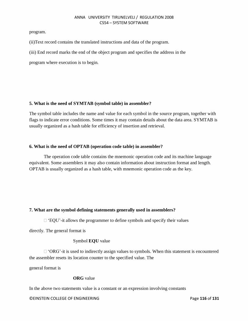
ANNA UNIVERSITY TIRUNELVELI / REGULATION 2008 CS54 – SYSTEM SOFTWARE
©EINSTEIN COLLEGE OF ENGINEERING Page 116 of 131
program.
(ii)Text record contains the translated instructions and data of the program.
(iii) End record marks the end of the object program and specifies the address in the
program where execution is to begin.
5. What is the need of SYMTAB (symbol table) in assembler?
The symbol table includes the name and value for each symbol in the source program, together with
flags to indicate error conditions. Some times it may contain details about the data area. SYMTAB is
usually organized as a hash table for efficiency of insertion and retrieval.
6. What is the need of OPTAB (operation code table) in assembler?
The operation code table contains the mnemonic operation code and its machine language
equivalent. Some assemblers it may also contain information about instruction format and length.
OPTAB is usually organized as a hash table, with mnemonic operation code as the key.
7. What are the symbol defining statements generally used in assemblers?
„EQU‟-it allows the programmer to define symbols and specify their values
directly. The general format is
Symbol EQU value
„ORG‟-it is used to indirectly assign values to symbols. When this statement is encountered
the assembler resets its location counter to the specified value. The
general format is
ORG value
In the above two statements value is a constant or an expression involving constants

ANNA UNIVERSITY TIRUNELVELI / REGULATION 2008 CS54 – SYSTEM SOFTWARE
©EINSTEIN COLLEGE OF ENGINEERING Page 117 of 131
and previously defined symbols.
8. Define relocatable program.
An object program that contains the information necessary to perform required modification
in the object code depends on the starting location of the program during load time is known as
relocatable program.
9. Differentiate absolute expression and relative expression.
If the result of the expression is an absolute value (constant) then it is known as absolute
expression.
Eg: BUFEND – BUFFER
If the result of the expression is relative to the beginning of the program then it is known as
relative expression. Label on instructions and data areas and references to the location counter values
are relative terms.
Eg: BUFEND + BUFFER
10. Write the steps required to translate the source program to object program.
Convert mnemonic operation codes to their machine language equivalents.
Convert symbolic operands to their equivalent machine addresses
Build the machine instruction in the proper format.
Convert the data constants specified in the source program into their internal machine
representation
Write the object program and assembly listing.
11. What is the use of the variable LOCCTR (location counter) in assembler?
This variable is used to assign addresses to the symbols. LOCCTR is initialized to the
beginning address specified in the START statement. After each source statement is processed the
length of the assembled instruction or data area to be generated is added to LOCCTR and hence
whenever we reach a label in the source program the current value of LOCCTR gives the address
associated with the label.

ANNA UNIVERSITY TIRUNELVELI / REGULATION 2008 CS54 – SYSTEM SOFTWARE
©EINSTEIN COLLEGE OF ENGINEERING Page 118 of 131
12. Define load and go assembler.
One pass assembler that generates their object code in memory for immediate execution is
known as load and go assembler. Here no object programmer is written out and hence no need for
loader.
13. What are the two different types of jump statements used in MASM assembler?
Near jump
A near jump is a jump to a target in the same segment and it is assembled by using a current code
segment CS.
Far jump
A far jump is a jump to a target in a different code segment and it is assembled by using different
segment registers.
14. What is the use of base register table in AIX assembler?
A base register table is used to remember which of the general purpose registers are currently
available as base registers and also the base addresses they contain. USING statement causes entry to
the table and .DROP statement removes the corresponding table entry.
15. Differentiate the assembler directives RESW and RESB.
RESW –It reserves the indicated number of words for data area.
Eg: 10 1003 THREE RESW 1
In this instruction one word area (3 bytes) is reserved for the symbol THREE. If the
memory is byte addressable then the address assigned for the next symbol is 1006.
RESB –It reserves the indicated number of bytes for data area.
Eg: 10 1008 INPUT RESB 1
In this instruction one byte area is reserved for the symbol INPUT .Hence the address assigned for
the next symbol is 1009.

ANNA UNIVERSITY TIRUNELVELI / REGULATION 2008 CS54 – SYSTEM SOFTWARE
©EINSTEIN COLLEGE OF ENGINEERING Page 119 of 131
16. Define modification record and give its format.
This record contains the information about the modification in the object code during
program relocation. The general format is
Col 1 M
Col 2-7 Starting location of the address field to be modified relative to the beginning of the
program
Col 8-9 length of the address field to be modified in half bytes.
17. Write down the pass numbers (PASS 1/ PASS 2) of the following activities that occur in a
two pass assembler:
a. Object code generation
b. Literals added to literal table
c. Listing printed
d. Address location of local symbols
Answer:
a. Object code generation - PASS 2
b. Literals added to literal table – PASS 1
c. Listing printed – PASS2
d. Address location of local symbols – PASS1
18. What is meant by machine independent assembler features?
The assembler features that do not depend upon the machine architecture are known as
machine independent assembler features.
Eg: program blocks, Literals.
ANNA UNIVERSITY TIRUNELVELI / REGULATION 2008 CS54 – SYSTEM SOFTWARE
©EINSTEIN COLLEGE OF ENGINEERING Page 120 of 131
19. How the register to register instructions are translated in assembler?
In the case of register to register instructions the operand field contains the register name.
During the translation first the object code is converted into its corresponding machine language
equivalent with the help of OPTAB. Then the SYMTAB is searched for the numeric equivalent of
register and that value is inserted into the operand field.
Eg: 125 1036 RDREC CLEAR X B410
B4-macine equivalent of the opcode CLEAR
10-numeric equivalent of the register X.
20. What is meant by external references?
Assembler program can be divided into many sections known as control sections and each
control section can be loaded and relocated independently of the others. If the instruction in one
control section needs to refer instruction or data in another control section the assembler is unable to
process these references in normal way. Such references between controls are called external
references.
21. Define control section.
A control section is a part of the program that maintains its identity after assembly; each
control section can be loaded and relocated independently of the others. Control sections are most
often used for subroutines. The major benefit of using control sections is to increase flexibility.
22. What is the difference between the assembler directive EXTREF and EXTDEF.
EXTDEF names external symbols that are defined in a particular control section and may be
used in other sections.
EXTREF names external symbols that are referred in a particular control section and defined
in another control section.
23. Give the general format of define record.

ANNA UNIVERSITY TIRUNELVELI / REGULATION 2008 CS54 – SYSTEM SOFTWARE
©EINSTEIN COLLEGE OF ENGINEERING Page 121 of 131
This record gives information about external symbols that are defined in a particular control
section. The format is
Col 1 D
Col 2-7 name of external symbol defined in this control section
Col 8-13 relative address of the symbol with in this control section
Col 14-73 name and relative address for other external symbols.
24. Give the use of assembler directive CSECT and USE
CSECT - used to divide the program into many control sections
USE – used to divide the program in to many blocks called program blocks
25. What is the use of the assembler directive START?
The assembler directive START gives the name and starting address of the program. The
format is
PN START 1000
Here
PN – Name of the program
1000 - Starting address of the program.
UNIT III - LOADERS AND LINKERS
1. What are the basic functions of loaders?
Loading – brings the object program into memory for execution

ANNA UNIVERSITY TIRUNELVELI / REGULATION 2008 CS54 – SYSTEM SOFTWARE
©EINSTEIN COLLEGE OF ENGINEERING Page 122 of 131
Relocation – modifies the object program so that it can be loaded at an address different
from the location originally specified
Linking – combines two or more separate object programs and also supplies the information
needed to reference them.
2. Define absolute loader.
The loader, which is used only for loading, is known as absolute loader.
e.g. Bootstrap loader
3. What is meant by bootstrap loader?
This is a special type of absolute loader which loads the first program to be run by the
computer. (usually an operating system)
4. What are relative (relocative) loaders?
Loaders that allow for program relocation are called relocating (relocative) loaders.
5. What is the use of modification record?
Modification record is used for program relocation. Each modification record specifies the starting
address and the length of the field whose value is to be altered and also describes the modification to
be performed.
6. What are the 2 different techniques used for relocation?
Modification record method and Relocation bit method.
7. Define Relocation bit method.
If the relocation bit corresponding to a word of object code is set to 1, the program‟s starting
address is to be added to this word when the program is relocated. Bit value 0 indicates no
modification is required.

ANNA UNIVERSITY TIRUNELVELI / REGULATION 2008 CS54 – SYSTEM SOFTWARE
©EINSTEIN COLLEGE OF ENGINEERING Page 123 of 131
8. Define bit mask.
The relocation bits are gathered together following the length indicator in each text record
and which is called as bit mask. For e.g. the bit mask FFC (111111111100) specifies that the first 10
words of object code are to be modified during relocation.
9. What is the need of ESTAB?
It is used to store the name and address of the each external symbol. It also indicates in which
control section the symbol is defined.
10. What is the use of the variable PROGADDR?
It gives the beginning address in memory where the linked program is to be loaded. The
starting address is obtained from the operating system.
11. Write the two passes of a linking loader.
Pass1: assigns address to all external symbols
Pass2: it performs actual loading, relocation and linking.
12. Define automatic library search.
In many linking loaders the subroutines called by the program being loaded are automatically
fetched from the library, linked with the main program and loaded. This feature is referred to as
automatic library search.
13. List the loader options INCLUDE &DELETE.
The general format of INCLUDE is
INCLUDE program_name (library name)
This command directs the loader to read the designated object program from a library and
treat it as the primary loader input.
The general format of DELETE command is
DELETE Csect-name

ANNA UNIVERSITY TIRUNELVELI / REGULATION 2008 CS54 – SYSTEM SOFTWARE
©EINSTEIN COLLEGE OF ENGINEERING Page 124 of 131
It instructs the loader to delete the named control sections from the sets of programs loaded.
14. Give the functions of the linking loader.
The linking loader performs the process of linking and relocation. It includes the operation of
automatic library search and the linked programs are directly loaded into the memory.
15. Define dynamic linking.
If the subroutine is loaded and linked to the program during its first call (run time), then it is
called as dynamic loading or dynamic linking.
16. Write the advantage of dynamic linking.
It has the ability to load the routine only when they are needed.
The dynamic linking avoids the loading of entire library for each execution.
17. What is meant by static executable and dynamic executable?
In static executable, all external symbols are bound and ready to run. In dynamic executables
some symbols are bound at run time.
18. What is shared and private data?
The data divided among processing element is called shared data. If the data is not shared among
processing elements then it is called private data.
20. Write the absolute loader algorithm.
Begin Read Header record
Verify program name and length Read first text record
While record type != „E‟ do
Begin Move object code to specified location in memory
Read next object program record
End Jump to address specified in End record
End
UNIT IV - MACRO PROCESSORS
1. Define macro processor.
Macro processor is system software that replaces each macroinstruction with the
corresponding group of source language statements. This is also called as expanding of macros.

ANNA UNIVERSITY TIRUNELVELI / REGULATION 2008 CS54 – SYSTEM SOFTWARE
©EINSTEIN COLLEGE OF ENGINEERING Page 125 of 131
2. What do macro expansion statements mean?
These statements give the name of the macroinstruction being invoked and the arguments to
be used in expanding the macros. These statements are also known as macro call.
3. What are the directives used in macro definition?
MACRO - it identifies the beginning of the macro definition
MEND - it marks the end of the macro definition
4. What are the data structures used in macro processor?
DEFTAB – the macro definitions are stored in a definition table i.e. it contains a macro
prototype and the statements that make up the macro body.
NAMTAB – it is used to store the macro names and it contains two pointers for each macro
instruction which indicate the starting and end location of macro definition
DEFTAB. it also serves as an index to DEFTAB
ARGTAB – it is used to store the arguments during the expansion of macro invocations.
5. Define conditional macro expansion.
If the macro is expanded depends upon some conditions in macro definition (depending on
the arguments supplied in the macro expansion) then it is called as conditional macro expansion.
6. What is the use of macro time variable?
Macro time variable can be used to store working values during the macro expansion. Any
symbol that begins with the character & and then is not a macro instruction parameter is assumed to
be a macro time variable.
7. What are the statements used for conditional macro expansion?
ANNA UNIVERSITY TIRUNELVELI / REGULATION 2008 CS54 – SYSTEM SOFTWARE
©EINSTEIN COLLEGE OF ENGINEERING Page 126 of 131
IF-ELSE-ENDIF statement
WHILE-ENDW statement
8. What is meant by positional parameters?
If the parameters and arguments were associated with each other according to their positions
in the macro prototype and the macro invocation statement, then these parameters in macro
definitions are called as positional parameters.
9. Consider the macro definition
#define DISPLAY (EXPR) Printf (“EXPR = %d\n”, EXPR)
Expand the macro instruction DISPLAY (ANS)
Ans.: Printf (“EXPR = %d\n”, ANS)
10. What are known as nested macro call?
The statement, in which a macro calls on another macro, is called nested macro all. In the
nested macro call, the call is done by outer macro and the macro called is the inner macro.
11. How the macro is processed using two passes?
Pass1: processing of definitions
Pass 2:actual-macro expansion.
12. Give the advantage of line by line processors.
It avoids the extra pass over the source program during assembling.
It may use some of the utility that can be used by language translators so that can be loaded
once.
13. What is meant by line by line processor?
This macro processor reads the source program statements, process the statements and then the
output lines are passed to the language translators as they are generated, instead of being written in
an expanded file.

ANNA UNIVERSITY TIRUNELVELI / REGULATION 2008 CS54 – SYSTEM SOFTWARE
©EINSTEIN COLLEGE OF ENGINEERING Page 127 of 131
14. Give the advantages of general-purpose macro processors.
The programmer does not need to learn about a macro facility for each compiler.
Overall saving in software development cost and maintenance cost.
15. What is meant by general-purpose macro processors?
The macro processors that are not dependent on any particular programming language, but
can be used with a variety of different languages are known as general purpose macro processors.
Eg. The ELENA macro processor.
16. What are the important factors considered while designing general purpose macro
processors?
comments
grouping of statements
tokens
syntax used for macro definitions
17. What is the symbol used to generate unique labels?
$ symbol is used in macro definition to generate unique symbols. Each macro
expansion the $ symbol is replaced by $XX, where XX is the alpha numeric character.
18. How the nested macro calls are executed?
The execution of nested macro call follows the LIFO rule. In case of nested macro calls the
expansion of the latest macro call is completed first.
19. Mention the tasks involved in macro expansion.
identify the macro calls in the program
the values of formal parameters are identified
maintain the values of expansion time variables declared in a macro
expansion time control flow is organized
determining the values of sequencing symbols
expansion of a model statement is performed
20. How to design the pass structure of a macro assembler?

ANNA UNIVERSITY TIRUNELVELI / REGULATION 2008 CS54 – SYSTEM SOFTWARE
©EINSTEIN COLLEGE OF ENGINEERING Page 128 of 131
To design the structure of macro-assembler, the functions of macro preprocessor and the
conventional assembler are merged. After merging, the functions are structured into passes of the
macro assembler.
UNIT V - TEXT EDITORS
1. Define interactive editor?
An interactive editor is a computer program that allows a user to create and revise a
target document. The term document includes objects such as computer programs, text,
equations, tables, diagrams, line art, and photographs anything that one might find on a printed
page.
2. What are the tasks performed in the editing process?
4 tasks
Select the part of the target document to be viewed and manipulated.
Determine how to format this view on-line and how to display it.
Specify and execute operations that modify the target document.
Update the view appropriately.
3. What are the three categories of editor’s devices?
Text device/ String devices
Button device/Choice devices
Locator device
4. What is the function performed in editing phase?
In the actual editing phase, the target document is created or altered with a set of operations
such as insert, delete, replace, move and copy.
5. Define Locator device?
Locator devices are two-dimensional analog-to-digital converters that position a cursor symbol on
the screen by observing the user‟s movement of the device. The most common such devices for
editing applications are the mouse and the data tablet.
6. What is the function performed in voice input device?
Voice-input devices, which translate spoken words to their textual equivalents, may prove to
be the text input devices of the future. Voice recognizers are currently available for command input
on some systems.
7. What are called tokens?

ANNA UNIVERSITY TIRUNELVELI / REGULATION 2008 CS54 – SYSTEM SOFTWARE
©EINSTEIN COLLEGE OF ENGINEERING Page 129 of 131
The lexical analyzer tracks the source program one character at a time by making the source
program into sequence of atomic units is called tokens.
8. Name some of typical tokens.
Identifiers, keywords, constants, operators and punctuation symbols such as commas and
parentheses are typical tokens.
9. What is meant by lexeme?
The character that forms a token is said to be a lexeme.
10. Mention the main disadvantage of interpreter.
The main disadvantage of interpreter is that the execution time of interpreted program is
slower than that of a corresponding compiled object program.
11. What is meant by code optimization?
The code optimization is designed to improve the intermediate code, which helps the object
program to run faster and takes less space.
12. What is error handler?
The error handler is used to check if there is an error in the program. If any error, it should
warn the programmer by instructions to proceed from phase to phase.
13. Name some of text editors.
line editors
stream editors
screen editors
word processors
structure editors
14. What for debug monitors are used?
Debug monitors are used in obtaining information for localization of errors.
15. Mention the features of word processors.
moving text from one place to another
merging of text
searching
word replacement
16. What are the phases in performing editing process?

ANNA UNIVERSITY TIRUNELVELI / REGULATION 2008 CS54 – SYSTEM SOFTWARE
©EINSTEIN COLLEGE OF ENGINEERING Page 130 of 131
Traveling phase
Filtering phase
Formatting phase
Editing phase
17. Define traveling phase.
The phase specifies the region of interest. Traveling is achieved using operations such as next
screenful, bottom, find pattern.
18. Filtering phase.
The selection of what is to be viewed and manipulated in given by filtering.
19. Editing phase
In this phase, the target document is altered with the set of operations such as insert, delete,
replace, move and copy.
20. Define user interface?
User interface is one, which allows the user to communicate with the system in order to
perform certain tasks. User interface is generally designed in a computer to make it easier to use.
21. Define input device?
Input device is an electromechanical device, which accepts data from the outside world and
translates them into a form, which the computer can interpret.
22. Define output devices
Output devices help the user to view the elements being edited and the results of the editing
operations.
23. What are the methods in Interaction language of a text editor?
Typing –oriented or text command oriented method
Function key interfaces
Menu oriented method

ANNA UNIVERSITY TIRUNELVELI / REGULATION 2008 CS54 – SYSTEM SOFTWARE
©EINSTEIN COLLEGE OF ENGINEERING Page 131 of 131
24. Define interactive debugging systems.
An interactive debugging system provides programmers with facilities that aid in the testing
and debugging of programs.
Debugging functions and capabilities
Relationship with other parts of the system
User interface criteria.
25. Define editor structure.
The command language processor accepts input from the users input devices and analyzes
the tokens and syntactic structure of the commands.
26. Give the components of editor structure
4 components
Editing component
Traveling component
Viewing component
Display component
27. What are the basic types of computing environments used in editor’s functions?
Editor‟s function in three basic types of computing environments
i. Time sharing ii. Stand-alone iii. Distributed