CS3210: GIS Lab 6: ArcGIS Network Analyst Tutorial - Aston University

1

Copyright Aston University. Materials developed by Laurence Chittock for module CS3210.

CS3210: GIS Lab 6: ArcGIS Network Analyst Tutorial

This lab will demonstrate the networking and routing capabilities in ArcGIS on road and rail data in the West Midlands.

You will learn how to set layer symbology, build networks and calculate the fastest route between two points. Finally, you will investigate the Midland Metro route, and make decisions on potential new stops based on their accessibility.

Firstly, download the data from the lab page of the wiki (Lab 6)

and extract the folder with the data inside.

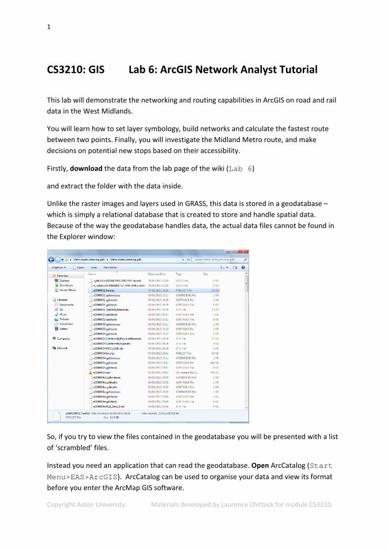
Unlike the raster images and layers used in GRASS, this data is stored in a geodatabase – which is simply a relational database that is created to store and handle spatial data. Because of the way the geodatabase handles data, the actual data files cannot be found in the Explorer window:

So, if you try to view the files contained in the geodatabase you will be presented with a list of ‘scrambled’ files.

Instead you need an application that can read the geodatabase. Open ArcCatalog (Start Menu>EAS>ArcGIS). ArcCatalog can be used to organise your data and view its format before you enter the ArcMap GIS software.

2


Navigate to the geodatabase:

Within the database you will see 3 subfolders, called ‘Feature Datasets’. These folders can help separate and organise your data and can also contain spatial reference information.

Go into the Metro_Line dataset. Here you will see the GIS layers which make up the Midland Metro. You can also view the data in ArcCatalog (but not edit).

Click on the Metro stops file and select Preview.

3


This shows the geographic view. You can also explore the attribute table by clicking on the dropdown box at the bottom: Preview: Geography. Change the selection to Table. This shows you the metadata for the Metro stops, with each stop entered as a separate record.

Viewing data and changing the symbology

Whilst ArcCatalog is useful for viewing and managing data, you cannot change its appearance or run many GIS tools. To edit the data and display it in a cartographic format, use ArcMap (Start Menu>EAS>ArcGIS) – and choose create ‘Blank Map’.

To view data in ArcMap, add it into the Layer Window. This can either be done by dragging the files from ArcCatalog or using the ‘Add Data’ button.

Add in the Metro Line and Metro Stops layers. Similarly to ArcCatalog, the data appears in the display window – except this time you can view more than one layer at a time.

To navigate around the data you can use the following toolbar:

The first two buttons allow you to zoom in and out, the 3rd is a pan tool and the 4th sets the zoom such that all of your data is in view. The ‘i’ button allows you to query individual features and bring up their attribute information.

Layer Window

4


One of the advantages of ArcGIS is that you can display geographic data and produce professional looking cartographic maps (as opposed to GRASS, which is mainly used just as an analytical tool). Each data layer’s symbology can be amended to give it some cartographic meaning. Double click on the Metro Lines layer (the layer name in the Layer Window) and navigate to the ‘Symbology’ tab.

Here, you can see what symbol currently defines this layer (in this case, a single coloured line). Click on this button to change the symbol to something more appropriate. You are presented with a list of options – you can select the line you want and amend its colour and width. Because this layer is showing the Metro rail line – select the ‘Railroad’ symbol (make it wider if you wish) and click OK. The Metro route now appears as a solid black line with interspersed black dashes – which is commonly used (and therefore recognised) to represent railway lines.

It is also possible to display different symbols for data within the same layer (which have different data attributes). To view the metadata for any layer, right click and select ‘Open Attribute Table’. Open the attribute table for the Metro stops and expand if necessary to see all the data.

5


This is the same data you saw in ArcCatalog. Each stop has been given a name, a status and a wait time (i.e. how long the train stops at the platform). Under Status, you will notice that some of the stops are listed as current and some as proposed.

It may be desirable to display this information in the map view. Navigate to the Metro Stops layer symobology. Instead of changing the symbol for all the features (stops), you wish to display them as different categories. Select ‘Categories’ on the left hand side.

6


Under the ‘Value Field’ dropdown, select Status (the field which distinguishes your data into categories). Click ‘Add All Values’ at the bottom – and you will see a separate symbol has been added for Proposed stops and Current ones. Double click on the Current symbol to change it.

You can now change the symbol to something you think appropriate – which will represent all current Metro stops.

As well as the standard symbols available in the first window, ESRI holds a massive library of other symbols which may be more suitable. If you type ‘train’ in the search window at the top – you will be presented with symbols which match this search. At the bottom of this list is a symbol which looks a bit like a tram. Select this if you wish, or something different if you deem it appropriate.

To distinguish between Current and Proposed stops, you may wish to change the size and colour of each symbol. For this tram symbol, you can change the colour by clicking on ‘Edit Symbol…’ and selecting a different colour and amending the size. Do the same for the Proposed stops so that they can be distinguished. In the main symbology window, you can deselect ‘<all other values>’ – as, in this case, there is no other data in the layer.

At this point, you have not edited any data (merely changed its appearance). Save the map at this point and you will save the changes you have made to the symbology. NB. When you save a map in ArcGIS, it saves just the map view only – that is, a list of the data which is

7


contained within the map and the way it is displayed. The data iteself is not saved in the map, rather the map file contains a pointer to the data telling it where it is stored. Every time you re-open your map, it will attempt to find the data in the location it was last saved (so if you move the data folder, the map will not be able to find the data – although the symbology etc will remain). This can be rectified by right clicking on the unfound layers and selecting Data>Repair Data Source.

Next, you will edit some of the data using ArcCatalog. Because ArcGIS places locks on the data whilst it is open, you can often not edit data that is open twice (even if the applications using it are ArcMap and ArcCatalog!). Therefore, once you have saved, Close ArcMap.

8


Building a Network

Open ArcCatalog and navigate to the Metro geodatabase and select the ‘Roads’ dataset. Here you will see a set of different road layers. Preview their appearance if you wish.

If you were to add these layers into ArcMap as they are, they will appear and be analysed as separate layers, i.e. ArcGIS doesn’t currently know that the A roads are in some way connected to the B roads. To analyse all the roads as one layer, and to be able to perform routing tasks you first need to build a network and tell ArcGIS how your data is connected.

See the link below for a description of the possibilities within the Arc Network Analyst.

http://resources.arcgis.com/en/help/main/10.1/index.html#/What_is_the_ArcGIS_Network_Analyst_extension/004700000001000000/

In particular, it describes a network as follows:

A network is a system of interconnected elements, such as edges (lines) and connecting junctions (points), that represent possible routes from one location to another. People, resources, and goods tend to travel along networks: cars and trucks travel on roads, airliners fly on predetermined flight paths, oil flows in pipelines. By modeling potential travel paths with a network, it is possible to perform analyses related to the movement of the oil, trucks, or other agents on the network. The most common network analysis is finding the shortest path between two points.

By building a network, ArcGIS allows you to set an impedance to each of your features. Impedance, or cost, is often just represented as distance (in which case Arc calculates this automatically). However, in the case of a road network it may be desirable to set an impedance of time. For instance, if you have a 1km section of motorway and a 1km section of minor roads their distance impedance will be the same. However, if you are driving in a car the time it takes for you to travel each route will usually be much shorter if you take the motorway.

In ArcCatalog, inspect the metadata for some of the road layers (Select Preview, then preview Table). For each layer, the travel time (Time_to_tr) is contained for each road segment in decimal minutes, i.e. 8.25 = 8mins 15seconds. By comparing similar length road segments between the road types, you will notice the difference in travel time. The travel time contained in these layers is based solely on an averaged speed limit for each road type. However, it is also possible to contain temporal data to allow for congestion affects or add a delay to different types of junctions.

Q. Can you work out the average speed (mph) along an A road? Bear in mind, travel times are in minutes and distances are in metres.



9


Add the extension by clicking Customize > Extensions then checking 'Network Analyst'. In the Roads dataset in ArcCatalog, right click New>Network Dataset…

You are presented with a wizard that will build your network, based on the data and parameters you set. To learn more about the functions of this wizard and the use of each step, see: http://resources.arcgis.com/en/help/main/10.1/index.html#/Exercise_1_Creating_a_network_dataset/00470000005t000000/ However, since we are building a relatively simple network most steps can be skipped (or left as default).

Click Next to Enter a name for your network dataset.

Select All the data layers and click next.

Click Next a further 3 times until you see this screen:

This step contains the types of impedance you wish to use in your network. You will see that ‘Meters’ (i.e. distance) is already entered. To add an impedance of time, click Add…

You will then need to type the name of the field where this impedance is stored, in this case ‘Time_to_tr’. Also select the Units as Minutes. Click OK.

Click Next and then select ‘No’ to establishing driving directions (your network will still be able to calculate routes etc, it just won’t catalogue the name of each road along the route).

Click Finish and then ‘Yes’ when prompted.

http://resources.arcgis.com/en/help/main/10.1/index.html#/Exercise_1_Creating_a_network_dataset/00470000005t000000/

http://resources.arcgis.com/en/help/main/10.1/index.html#/Exercise_1_Creating_a_network_dataset/00470000005t000000/

10


Routing on a Network

You will notice that a new feature has been created – your Road Network dataset.

Re-open your saved map from earlier and add in the Road Network dataset.

When asked if you want to add in all the feature classes that participate in your Roads_ND network, select Yes.

Unfortunately, in doing so, your nice cartographic display from earlier has become cluttered and uninformative. This is because the network is made up by lots of junction points (the points at which join 2 roads together). However, at any time you can deselect layers from view by unticking them in the Layer Window. Deselect the layers Road_junctions, Roads_ND_Junctions and Roads_ND. Now, you are just left with the Metro line, stops and the roads. You may wish to change the symbol display for each of the roads (e.g., make Motorways light blue in colour and thicker).

Because your Road network is present in the Layer Window (even if it is deselected) you can now perform routing tasks. To do so, add the Network Analyst toolbar (under Customize>Toolbars).

11


From the dropdown menu select New Route. Then select the ‘Create Network Location Tool’ button (highlighted above). This allows you to place a start and end point for your route. Click and place 2 points on different sides of the map.

You now need to tell the software which impedance method to use. If it is not already selected, open the Network Analysis Window. This contains a list of the stops currently contained in the Route Analyst and also allows you to add any restrictions to your route (if they exist).

Open the Route Properties and navigate to the ‘Analysis Settings’ tab.

If it is not already selected, change the impedance to ‘Time_to_tr’ – the travel time impedance you created earlier.

Select Output Shape Type as ‘True Shape with Measures’.

On the ‘Accumulation’ tab, tick both boxes.

Click OK.

Open Network Analyst Window

Route Properties

12


In this example, you simply want to find the best route from A to B (the 2 stops you placed). Using the information contained in your network Arc will calculate the least cost route between the 2 points based on the time it takes to travel (in a car). To do this, click the ‘Solve’ button on the Network Analyst toolbar:

The quickest route between your 2 points is displayed. If you go back into Route Properties and change the impedance to Metres and then re-solve, you will probably find your route changes. Instead of finding the quickest route, Arc will now find the shortest route (which may well be along small minor roads). In both cases you can open the attribute table of the resultant routes layer and compare the Time and Length of each route.

NB. For those of you who drive a car in Birmingham you might be surprised by the speedy time it has calculated for your route! Bear in mind though that the travel times on the roads were set up to mirror optimal driving speeds and hence do not factor in congestion.

NB.2 In the screenshot above, the route shown is not actually possible in reality. Near the start of the route the path shown leads from an A road and joins up with the motorway at junction 8 of the M6. However, in reality there is no connection to an A road at jct 8 –this is the junction which connects to the M5 only. To rectify this you would have to edit the offending junction so that it had a restriction that did not allow the motorway to connect to the A road.

When you are done, you can remove the Route layer by right clicking on it and selecting ‘Remove’.

13


Location modelling set-up

As well as simple routing, the Network Analyst also allows you to work out much more complicated problems. For instance, in this example the Metro company wish to place an extra 4 stops along a proposed route. This route is an addition to the existing Midland Metro and will run from Birmingham Snow Hill, through the city centre, along the Hagley Road (A456) and then through Smethwick before re-joining the existing line at the Kenrick Park stop. The Metro company have identified a possible 8 new sites where they can build stops – but wish to choose only the 4 ‘best’ stops. They define the best 4 stops as those which capture the greatest amount of population – i.e. they wish to maximise their customer base. Typically, a large proportion of their current customers arrive at their local Metro stop on foot and as such they are only interested in finding potential customers who are within walking distance (1km).

To undertake this task you will need to know where the population centres are in the local vicinity. Typically, the best source for population data (and many other demographics) is the Census – see Appendix 1 for information on where to get this data.

For this task however, the data is already provided. In your map, add in the WestMids_Census_OA (within the Census dataset). This layer contains all the Output Areas, which are small Census zones, in the West Midlands region. If this layer obscures the rest of your data you can drag it to the bottom of the Layer Window. You can also make it semi-transparent if you wish by double-clicking and going to the Display tab. Set the transparency to 60% and also change the colour if you wish.

If you inspect this layer (either open the attribute table or examine one of the zones using the ‘i’ button) – you will see a large list of statistics. The field names contained here refer to various different types of Census information. A lookup to their meanings can be found here:

http://www.ons.gov.uk/ons/guide-method/census/census-2001/data-and-products/about-the-tables-and-products/types-of-table/standard-output-tables.xls

For this task however, the total population (KS0010001) will be sufficient. You will use this statistic to determine where people live and thus whether they are suitable customers for your new Metro route. To do this, you will need to determine the accessibility of each stop – that is, how many people can reach each stop by travelling along the road network. For instance, it is no use living 100m from a metro stop if there is no road or path to take you there, or if the only road available is a motorway which you cannot cross!

To determine how close people live to each Metro stop you will need to represent your population as demand points. The Network Analyst can only work out a route between 2



14


points, not an area and a point. To convert your Output Areas to points you will need to use the Feature-to-Point tool.

Under the Geoprocessing tab, select Search for Tools. In the search box, type in the tool you need and select Feature To Point (Data Management).

Select the Output Areas layer as your input. Choose a location and name for your output (place it in your geodatabase). If the data does not appear, add the data in from your saved location.

These points represent the centroid for each area. Effectively you have condensed the location of everyone within the same Output Area to a point. In this scenario, this is probably OK because OAs are quite small – and thus you are only moving people’s actual location a few hundred metres. However, there may be times where this is not so appropriate – it all depends on the modelling parameters, the decisions you are making and the processing power available.

Currently, you have population points for all OAs in the West Midlands. However, since you are only considering people who can walk to their nearest stop the majority of the West Midlands population can be excluded. To do this you wish to find out which centroids are near to the current and proposed Metro stops.

In the Search for Tools box, look for the Buffer (analysis) tool.

15


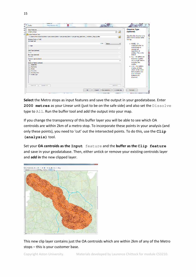
Select the Metro stops as input features and save the output in your geodatabase. Enter 2000 metres as your Linear unit (just to be on the safe side) and also set the Dissolve type to All. Run the buffer tool and add the output into your map.

If you change the transparency of this buffer layer you will be able to see which OA centroids are within 2km of a metro stop. To incorporate these points in your analysis (and only these points), you need to ‘cut’ out the intersected points. To do this, use the Clip (analysis) tool.

Set your OA centroids as the Input feature and the buffer as the Clip feature and save in your geodatabase. Then, either untick or remove your existing centroids layer and add in the new clipped layer.

This new clip layer contains just the OA centroids which are within 2km of any of the Metro stops – this is your customer base.

16


Choosing the best proposed stops

To choose the ‘best’ new stops for the Metro route, you will need to run a location-allocation model. This model will attempt to allocate demand points (OA centroids) to their nearest and most convenient Metro stop based on their location.

In the Network Analyst toolbar, choose New Location-Allocation. To learn more about location-allocation with ArcGIS, see: http://resources.arcgis.com/en/help/main/10.1/index.html#/Location_allocation_analysis/004700000050000000/

This tool allows you to enter a set of facilities (i.e. your Metro stops) and a set of demand points (OA centroids). In the Layer Window you will notice the Facilities are categorised as: Candidate, Chosen, Required or Competitor. In this example, you have a set of Required points (your current stops) and Candidate ones (proposed). The Network Anaylst recognises Required points with a 1 and Candidate points with a 0. If you open the Metro stops attribute table you will see this data has already been entered for you (under the FacilityType field).

To add in the Metro stops as facilities, right click on Facilities in the Network Analyst Window (not the Layer window) and click Load Locations. Fill out the form as shown below.

http://resources.arcgis.com/en/help/main/10.1/index.html#/Location_allocation_analysis/004700000050000000/

http://resources.arcgis.com/en/help/main/10.1/index.html#/Location_allocation_analysis/004700000050000000/

17


Choose Load from Metro stops. You can then amend the table below so that the StopName is entered for each facility. Also make sure the Facility Type is being read from the right field. Load in the locations.

The Metro stops will now appear as facilities and will have inherited the relevant symbology (i.e. either Required or Candidate).

You will also need to load in your demand points. Right click on Demand Points in the Network Analyst Window and click Load Locations.

Choose Load from your OA points clip layer. The name you set for each point is not too important here, but set it as a unique identifier – either ObjectID or Zone Code. It is important however to set the weight field for your demand points as this will determine how much importance (weight) the model assigns to each OA. Set the weight as KS0010001 – the population field from the Census.

Below this table you can set the ‘Location Position’. Currently it is set to Use Geometry – Search tolerance of 5000 metres. So the Network Analyst can calculate routes between 2 points, it has to place, or snap, each point to a position on the network. The search tolerance therefore, determines how far you are willing to move a point to place it on the network. In this case, it should be obvious that no point is further than 5km from a road – in fact it is much less – so set the search tolerance to 500 metres instead.

18


NB. If you were to leave the search tolerance as 5000 metres it would still locate the points in the same place, it would just take much longer for Arc to process this (effectively it finds all roads with 5km of each point and then calculates which is the closest).

Click OK to load in your demand points.

Occassionally, you may wish to set up restrictions or barriers in your model. These restrictions tell the model which part of your network cannot be traversed. In this case, you may wish to set the motorways layer as a barrier (since your customer base is travelling by foot). Right click on Line Barriers in the Network Analyst Window and select Load Locations. Choose your motorway layer and click OK.

Now you have loaded all the data into your model, you need to set up the parameters that it will use to solve the problem. In the Network Analyst Window click on the Location Allocation Properties icon. Navigate to the Analysis Settings tab. Set the impedance to Metres and also change the Travel from: to Demand to Facility.

NB. The reason you are using distance as the impedance here is because your customers are walking to their nearest Metro stop. The travel time you set up was for car drivers – and thus if you wanted to calculate the driving time towards stops you would use this. By setting the

19


impedance as distance you are assuming that the time it takes to walk somewhere is a direct function of the distance. This is probably true in most cases, especially in Birmingham which is largely flat – but in certain areas this may not be the case where walking up a hill takes significantly longer than travelling the same distance on flat land (‘anisotropy’!). There are also other factors which may affect walking times, such as crossing a busy road. This could be incorporated into your model, by adding a delay to certain road types or junctions – but for now it is safe to assume walking speed is constant.

Finally, navigate to the Advanced Settings tab. Here, you can define what sort of problem you want to solve and set the parameters for your model. For this task, Minimize Impedance is appropriate. You wish to choose the set of facilities which can capture the greatest demand (population weight) in the minimum distance. Explore the other problem types if you wish or use the ArcGIS 10.1 desktop help for more information.

The Facilities to Choose value reflects how many Metro stops you want the model to choose. The task asks you to find an additional 4 stops out of 8 proposed stops. However, you will still need to include the 27 other existing stops. If you did not you might potentially steal customers from one of your existing stops and assign them to a new stop. This is fine if

20


the new stop is closer – but it is assumed that people will still use the existing stops if this is more convenient. Since you set your existing stops to ‘Required’, the model will automatically choose these and then decide which are the best 4 additional stops.

The Impedance cutoff is the maximum distance you think people will be willing to walk to a metro stop. Therefore anyone beyond this distance will be excluded from the model. Set this value to 1000 metres, or something different if you think it appropriate. Click OK.

There’s one last thing to do before running the algorithm – we need to make sure that walking routes are realistic and don’t go along motorways! To stop people from being allocated to motorway segments, go to the ‘Network Locations’ tab and uncheck ‘Motorways’ as shown below:

You are now ready to solve your location allocation problem. Run Solve.

It might not be immediately obvious what has happened – so zoom in closer to some of the stops. You will notice that 4 of your proposed stops have changed their symbol to ‘Chosen’. The model has decided that this combination of stops captures the most number of people within your impedance cutoff. The lines spidering out from each stop indicate which OA points have been allocated to each stop.

See the next page for a larger image of how the result should look.

21


Take a look at the Facilities Attribute table. In this example the Bearwood, Five Ways, Hagley Road and Smethwick Cape Hill stops were chosen. These stops will serve the largest number of people within 1km. Changing your impedance cutoff or the number of facilities you choose will probably produce a different result. The important figures in this table are the ‘Demand Count’ and ‘Demand Weight’ fields. The new Bearwood stop captures demand

22


from 40 OA centroids – giving a total customer base of 11,300. The total number of customers captured by the 4 chosen stops will have been higher than any other combination possible – hence why these ones were deemed the ‘best’.

Q. What happens if you change the maximum impedance cutoff? Does this change your result?

23


Appendix 1 – Downloading Census data

To access Census data, visit:

Visit: http://casweb.mimas.ac.uk/

Here you can download data from any of the UK Census’ since 1971. Data from the 2011 Census is gradually being released and made available online – and they are now using a new website from where you can download this data: http://infuse.mimas.ac.uk/. However, the full datasets are not yet available – so we will stick to 2001 for now.

Login in to Casweb (if you have not already registered, then you will have to do so. Unfortunately, it takes a couple of days before your account is activated…)

Select 2001 Aggregate Statistics Datasets (with digital boundary data)

& Proceed to the 2001 Aggregate Statistics Datasets

You will now need to select the area you are interested in: which in this case is the West Midlands. Select lower geographies>tick F: West Midlands>Select Counties>tick 2E: West Midlands

You can now Select output level. At the bottom, tick OA and Select data…

http://casweb.mimas.ac.uk/

http://infuse.mimas.ac.uk/

24


At the ‘Key Statistics’ table at the bottom you can select all sorts of data from the Census, e.g. populations, age ranges, religion, occupation group, method of travel to work etc.

Select one you are interested in and ‘Display Table Layout’. This table shows you all the statistics that are available for that category.

This screenshot shows the Table layout for ‘Usual resident population’. If you select the ‘All people’ box, you will be given a statistical count of all the people who live in each Output Area.

In the top right, select ‘Get data’. You will then be able to select the format for your data – you can either select Plain text, which will give you the data in a table format, or select Digital Boundary Data which provides the data in a GIS format.

25


As well as the Census statistics, the Digital Boundary Data holds the shapes for each Output Area – thus giving them geographical context.

However, it may not always be possible to download data contained within GIS boundaries. In such cases, you will need to download a separate GIS boundary layer. This can be done from http://edina.ac.uk/ukborders/. Here, you can download digital boundary data for different geographic areas and output sizes across the whole UK. Once you have a GIS layer for the Census boundaries, you can join your statistical data (from a table) to this layer.

http://edina.ac.uk/ukborders/

Documents

CS3210: GIS Lab 6: ArcGIS Network Analyst Tutorial - Aston University