CS301 - Algorithms

CS301 - Algorithms

Fall 2006-2007

Hüsnü Yenigün

CS301 – Algorithms [ Fall 2006-

2007 ] 2

Contents About the course Introduction

What is an algorithm? Computational problems An instance of a problem Correctness of algorithms Loop invariant method for showing correctness of algorithms What does a better algorithm mean? Selecting the best algorithm Analysis of “Insertion Sort” algorithm Which running time – best, average, worst – should we use? Asymptotic analysis Divide and Conquer Analysis of divide and conquer algorithms

Growth of functions & Asymptotic notation O-notation (upper bounds) o-notation (upper bounds that are not tight) Ω-notation (lower bounds) ω-notation (lower bounds that are not tight) Θ-notation (tight bounds) Some properties of asymptotic notations Some complexity classes


2007 ] 3

About the course

Instructor Name: Hüsnü Yenigün Office: FENS 2094 Office Hours:

Walk-in: Thursdays 08:40-09:30 By appointment: any available time (please read the footnote)

http://people.sabanciuniv.edu/yenigun/calendar.php

TAs Name: Mahir Can Doğanay, Ekrem Serin Office: FENS xxxx Office Hours: to be decided


2007 ] 4

About the course

Evaluation: Exams:

1 Midterm (November 23, 2006 @ 09:40 – pending approval) 1 Final (to be announced by Student Resources) 1 Make-up (after the final exam) - You have to take exactly 2 of these 3 exams

(no questions asked about the missed exam)

- Make-up, if taken, counts as the missed exam

- If you take only one or none of these exams, the missing exam/exams is/are considered to be 0

Homework ~ 6-7

Weights of these grading itemswill be announced at the end ofthe semester.


2007 ] 5

About the course

Recitations: Problem solving Not regular Will be announced in advance

All communication through WebCT No e-mail to my personal account (you can send

me an e-mail to let me know that you’ve posted something on WebCT)


2007 ] 6

About the course

Course material

Textbook: Introduction to Algorithms

by Cormen et al.

Lecture notes:

ppt slides (will be made available on WebCT)


2007 ] 7

Why take this course?

Very basic – especially for CS and MSIE – and intellectually enlightening course

Get to know some common computational problems and their existing solutions

Get familiar with algorithm design techniques (that will help you come up with algorithms on your own)

Get familiar with algorithm analysis techniques (that will help you analyze algorithms to pick the most suitable algorithm)

Computers are not infinitely fast and memory is limited

Get familiar with typical problems and learn the bounds of algorithms (undecidability and NP-completeness)


2007 ] 8

Tentative Outline

Introduction Asymptotic Notation Divide and Conquer

Paradigm Recurrences Solving Recurrences Quicksort Sorting in linear time Medians and order

statistics Binary search trees Red-Black trees

Augmenting data structures

Dynamic programming Greedy algorithms Amortized Analysis B-Trees Graph algorithms Sorting Networks Computational Geometry Undecidability NP-Completeness


2007 ] 9

INTRODUCTION


2007 ] 10

What is an algorithm?

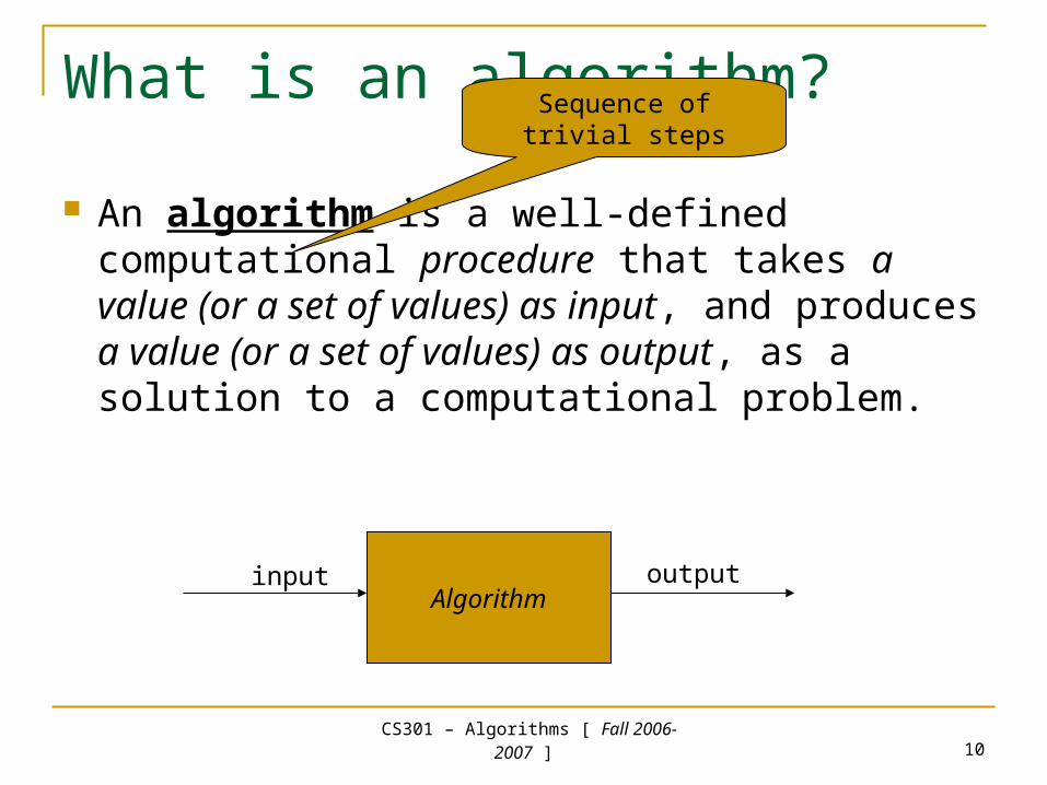
An algorithm is a well-defined computational procedure that takes a value (or a set of values) as input, and produces a value (or a set of values) as output, as a solution to a computational problem.

Sequence of trivial steps

Algorithminput output


2007 ] 11

The statement of the problem defines what is the relationship between the input and the output.

The algorithm defines a specific computational procedure that explains how this relationship will be realized.


2007 ] 12

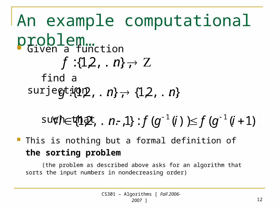
An example computational problem… Given a function

find a surjection

such that

},...,2,1{: nf

},...,2,1{},...,2,1{: nng

))1(())((:}1,...,2,1{ 11 igfigfni This is nothing but a formal definition of

the sorting problem (the problem as described above asks for an algorithm that sorts the input numbers

in nondecreasing order)


2007 ] 13

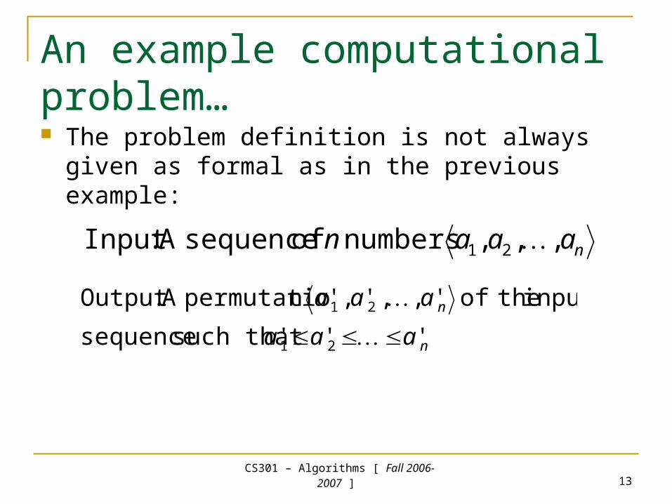
An example computational problem… The problem definition is not always given as formal

as in the previous example:

naaan ,,, numbers of sequenceA :Input 21

n

n

aaa

aaa

'''such that sequence

input theof ',,','n permutatioA :Output

21

21


2007 ] 14

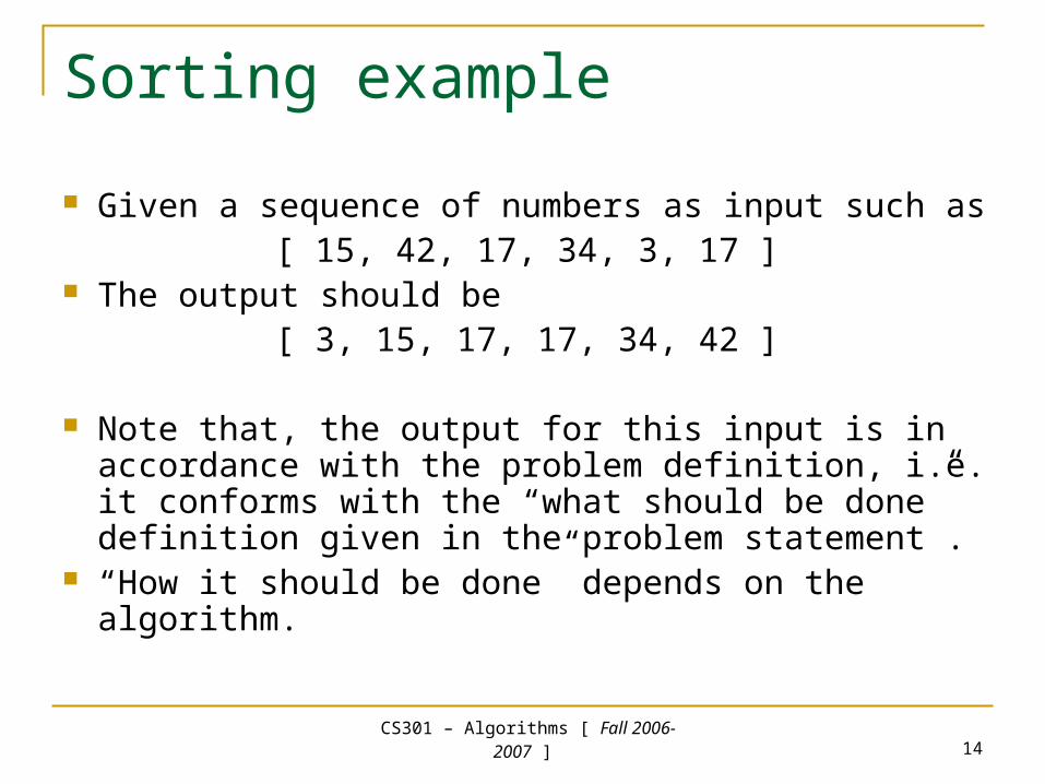
Sorting example

Given a sequence of numbers as input such as[ 15, 42, 17, 34, 3, 17 ]

The output should be [ 3, 15, 17, 17, 34, 42 ]

Note that, the output for this input is in accordance with the problem definition, i.e. it conforms with the “what should be done” definition given in the problem statement .

“How it should be done” depends on the algorithm.


2007 ] 15

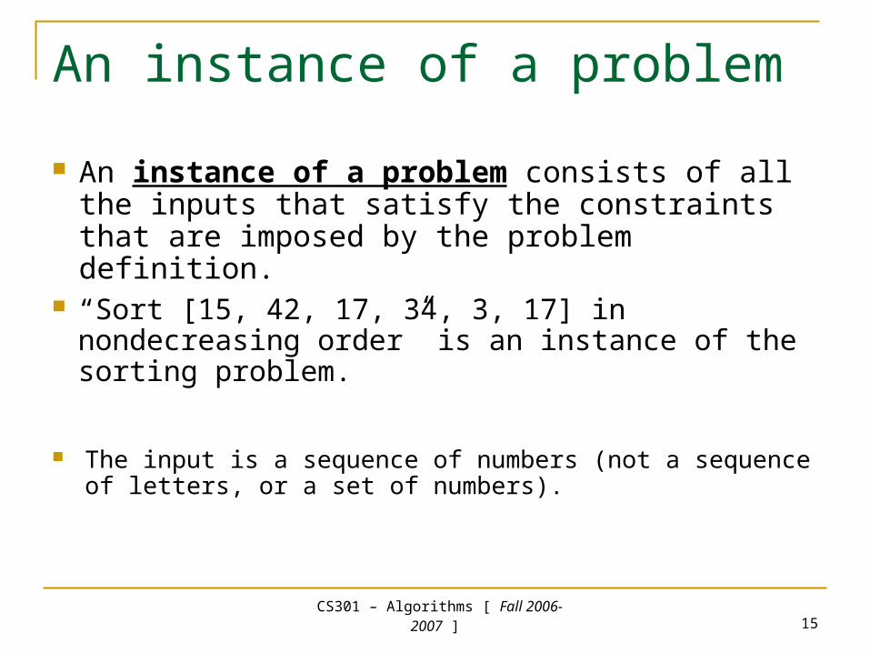
An instance of a problem

An instance of a problem consists of all the inputs that satisfy the constraints that are imposed by the problem definition.

“Sort [15, 42, 17, 34, 3, 17] in nondecreasing order” is an instance of the sorting problem.

The input is a sequence of numbers (not a sequence of letters, or a set of numbers).


2007 ] 16

Not the sorting problem again !!! Sorting is a fundamental operation in many

disciplines and it is used as a part of other algorithms.

A lot of research has been made on the sorting problem.

A lot of algorithms have been developed. It is a very simple and interesting problem to

explain basic ideas of algorithm design and analysis techniques.


2007 ] 17

Correctness of algorithms

An algorithm is correct if for every instance of the problem, it halts (terminates) producing the correct answer.

Otherwise (i.e. if there are some instances for which the algorithm does not halt, or it produces an incorrect answer), it is called an incorrect algorithm.

Surprisingly, incorrect algorithms are occasionally used in practice (e.g. primes problem)…


2007 ] 18

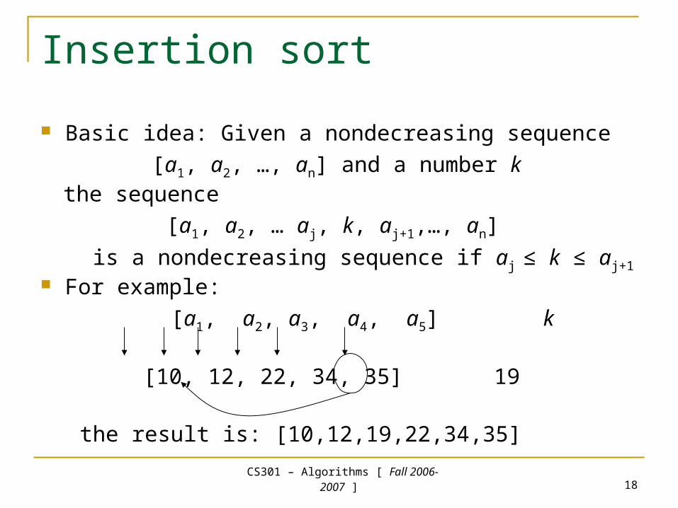
Insertion sort

Basic idea: Given a nondecreasing sequence

[a1, a2, …, an] and a number k the sequence

[a1, a2, … aj, k, aj+1,…, an]

is a nondecreasing sequence if aj ≤ k ≤ aj+1

For example:

[a1, a2, a3, a4, a5] k

[10, 12, 22, 34, 35] 19

the result is: [10,12,19,22,34,35]


2007 ] 19

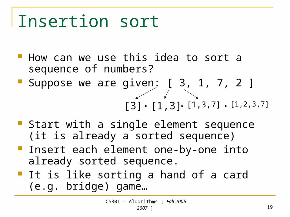
Insertion sort

How can we use this idea to sort a sequence of numbers?

Suppose we are given: [ 3, 1, 7, 2 ]

Start with a single element sequence (it is already a sorted sequence)

Insert each element one-by-one into already sorted sequence.

It is like sorting a hand of a card (e.g. bridge) game…

[3] [1,3] [1,3,7] [1,2,3,7]


2007 ] 20

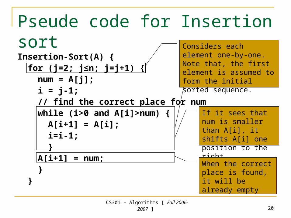
Pseude code for Insertion sortInsertion-Sort(A) { for (j=2; j≤n; j=j+1) { num = A[j]; i = j-1; // find the correct place for num while (i>0 and A[i]>num) { A[i+1] = A[i]; i=i-1; } A[i+1] = num; } }

Searches for the correct place to insert the next element.

If it sees that num is smaller than A[i], it shifts A[i] one position to the right

When the correct place is found, it will be already empty

Considers each element one-by-one. Note that, the first element is assumed to form the initial sorted sequence.


2007 ] 21

BREAK


2007 ] 22

Showing the correctness of Insertion Sort Note that, “Insertion-Sort” is an iterative

algorithm. Loop invariants is a widely used method to

show the correctness of iterative algorithms. A loop invariant is a boolean statement

that is correct for all the iterations of the loop. Loop invariant method is performed in 3

steps, and related to the mathematical induction proofs.


2007 ] 23

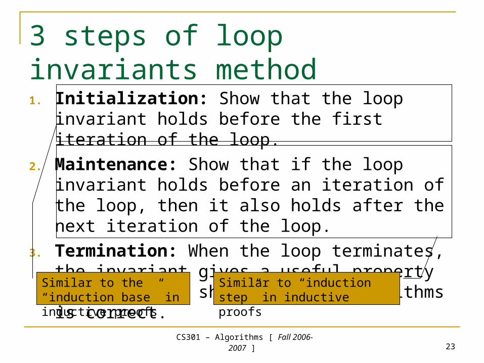
3 steps of loop invariants method1. Initialization: Show that the loop invariant

holds before the first iteration of the loop.

2. Maintenance: Show that if the loop invariant holds before an iteration of the loop, then it also holds after the next iteration of the loop.

3. Termination: When the loop terminates, the invariant gives a useful property that helps to show that the algorithms is correct.

Similar to the “induction base” in inductive proofs

Similar to “induction step” in inductive proofs


2007 ] 24

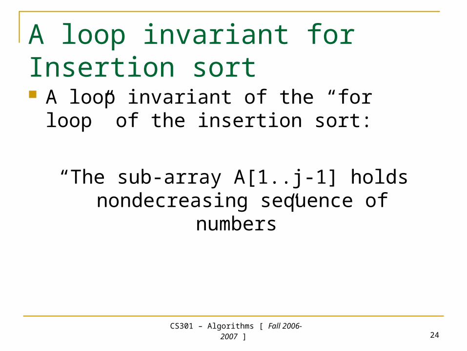
A loop invariant for Insertion sort A loop invariant of the “for loop” of the

insertion sort:

“The sub-array A[1..j-1] holds nondecreasing sequence of numbers”


2007 ] 25

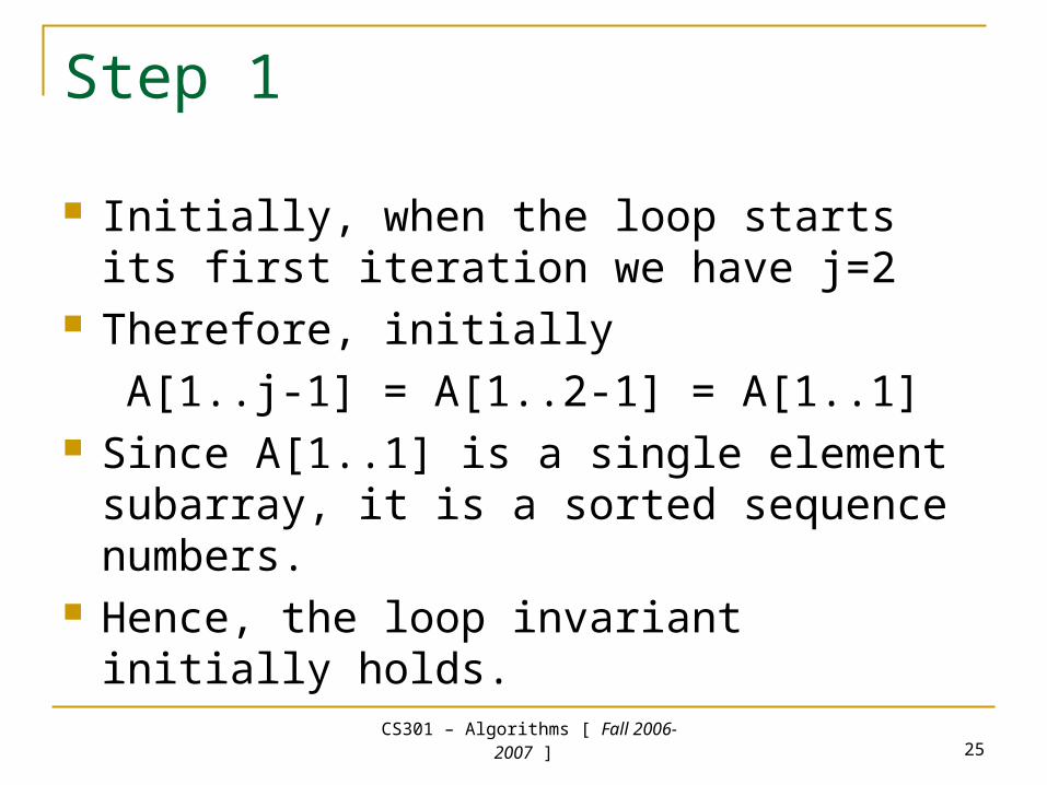
Step 1

Initially, when the loop starts its first iteration we have j=2

Therefore, initially

A[1..j-1] = A[1..2-1] = A[1..1] Since A[1..1] is a single element subarray, it

is a sorted sequence numbers. Hence, the loop invariant initially holds.


2007 ] 26

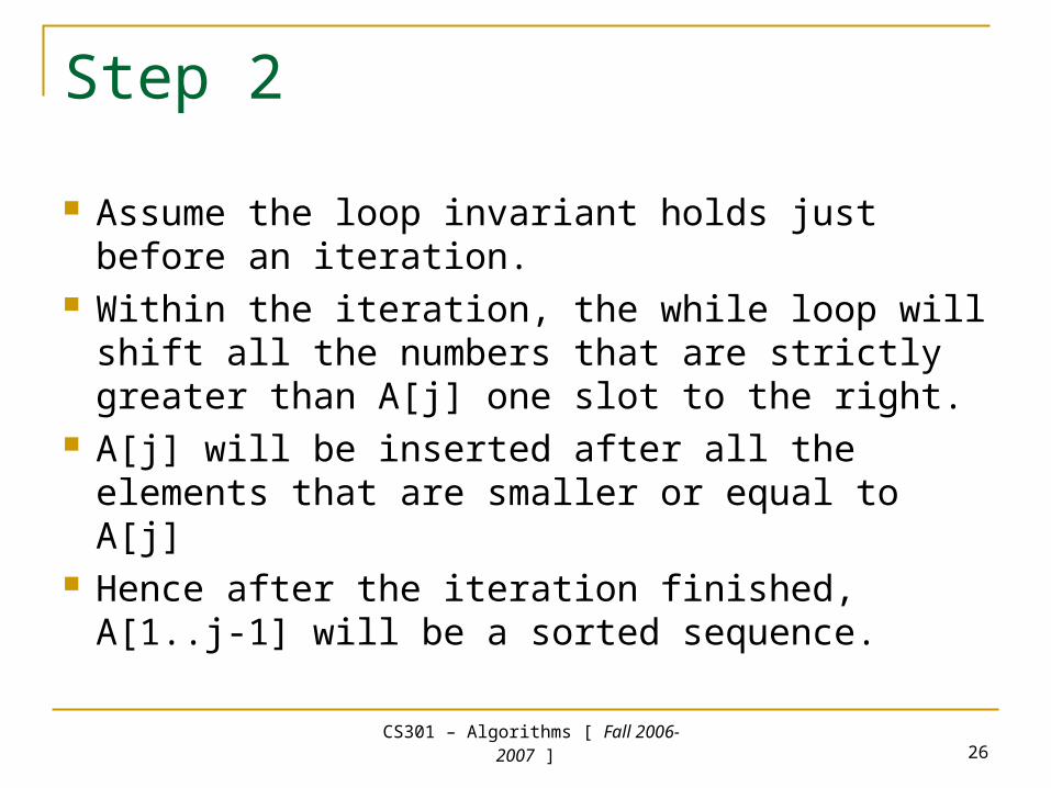
Step 2

Assume the loop invariant holds just before an iteration.

Within the iteration, the while loop will shift all the numbers that are strictly greater than A[j] one slot to the right.

A[j] will be inserted after all the elements that are smaller or equal to A[j]

Hence after the iteration finished, A[1..j-1] will be a sorted sequence.


2007 ] 27

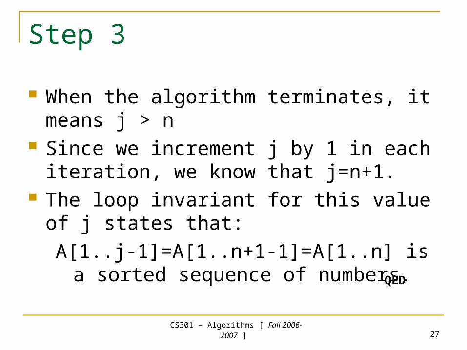
Step 3

When the algorithm terminates, it means j > n Since we increment j by 1 in each iteration,

we know that j=n+1. The loop invariant for this value of j states

that:

A[1..j-1]=A[1..n+1-1]=A[1..n] is a sorted sequence of numbers.

QED


2007 ] 28

Is Insertion sort the solution for the sorting problem? Insertion sort is only a solution for the

sorting problem. “But we’ve just proved that it works correctly

for all the input sequences. Why do we need other algorithms to solve the sorting problem?”

There may be other algorithms better than Insertion sort…


2007 ] 29

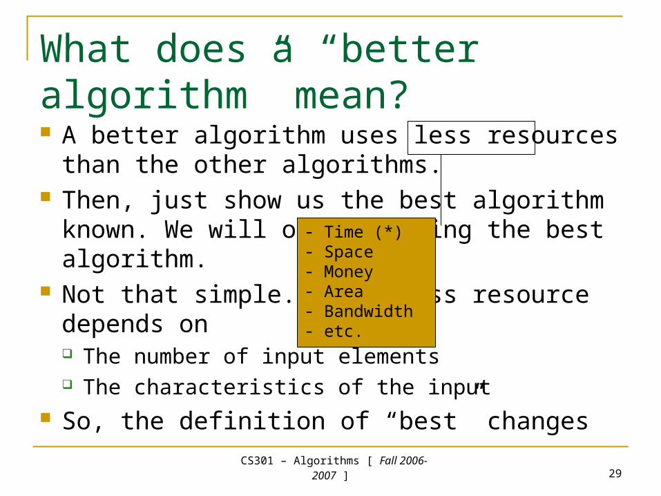
What does a “better algorithm” mean? A better algorithm uses less resources than

the other algorithms. Then, just show us the best algorithm known.

We will only be using the best algorithm. Not that simple. Using less resource depends

on The number of input elements The characteristics of the input

So, the definition of “best” changes

- Time (*)- Space- Money- Area- Bandwidth- etc.


2007 ] 30

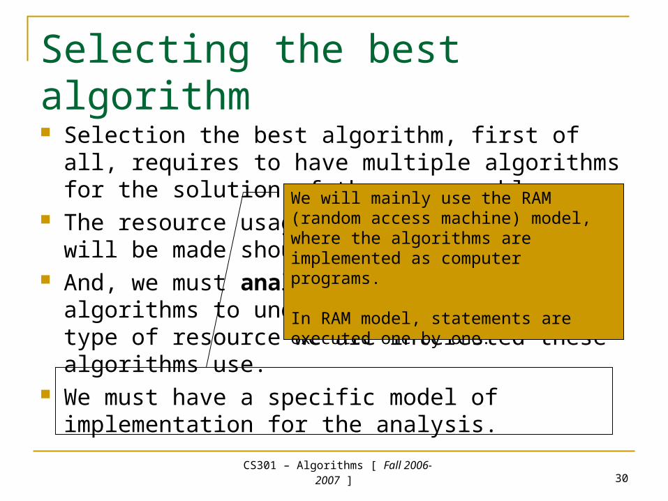
Selecting the best algorithm

Selection the best algorithm, first of all, requires to have multiple algorithms for the solution of the same problem.

The resource usage on which our selection will be made should be known.

And, we must analyze the available algorithms to understand how much of the type of resource we are interested these algorithms use.

We must have a specific model of implementation for the analysis.

We will mainly use the RAM (random access machine) model, where the algorithms are implemented as computer programs.

In RAM model, statements are executed one by one.


2007 ] 31

Analysis of Insertion sort

Time taken by Insertion sort depends on The number of elements to be sorted

10 elements vs. 1000 elements The nature of the input

already sorted vs. reverse sorted In general, the time taken by an algorithm

grows with the size of the input. Therefore, we describe the running time of an

algorithm as a function of the input size.


2007 ] 32

Definition of the input size

It depends on the problem. For sorting problem, it is natural to pick the

number of elements as the size of the input. For some problems, a single measure is not

sufficient to describe the size of the input. For example, for a graph algorithm, the size

of the graph is better described with the number of nodes and the number of edges given together.


2007 ] 33

Definition of the running time We can use a 1990 PC AT computer or a

contemporary supercomputer to execute an implementation of the algorithm.

A good programmer can implement the algorithm directly using assembly code, or a beginner programmer can implement it using a high level language and compile it using the worst compiler (which has no optimization).

So, the running time of a given algorithm seems to depend on certain conditions.


2007 ] 34

Definition of the running time Our notion of “running time” should be as

independent as possible from such consideration.

We will consider the “number of steps” on a particular input as the running time of an algorithm.

For the time being, let us assume that each step takes a constant amount of time.


2007 ] 35

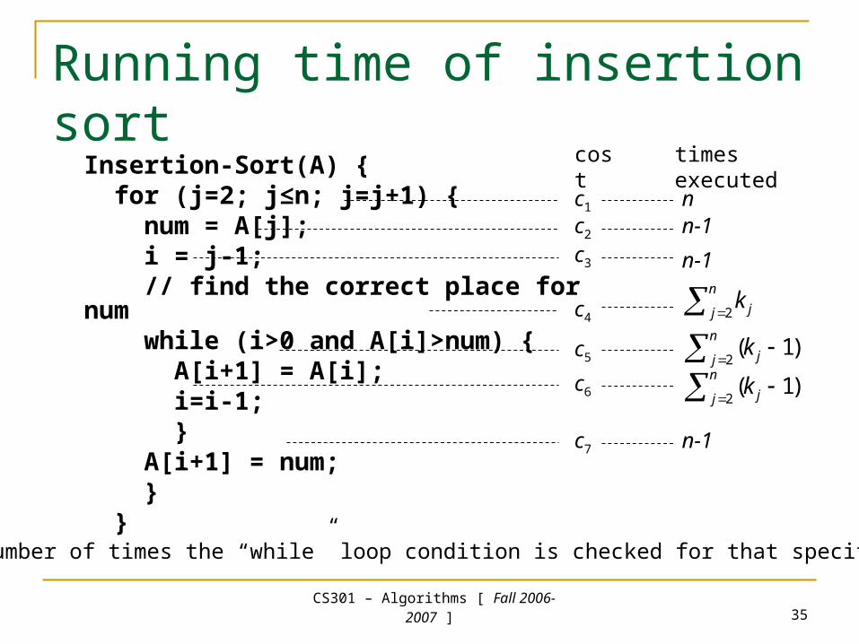
Running time of insertion sort

Insertion-Sort(A) { for (j=2; j≤n; j=j+1) { num = A[j]; i = j-1; // find the correct place for num while (i>0 and A[i]>num) { A[i+1] = A[i]; i=i-1; } A[i+1] = num; } }

cost times executed

c1

c2

c3

c4

c5

c6

c7

nn-1

n-1

n

j jk2

n

j jk2

)1(

n

j jk2

)1(

n-1

kj: the number of times the “while” loop condition is checked for that specific j value


2007 ] 36

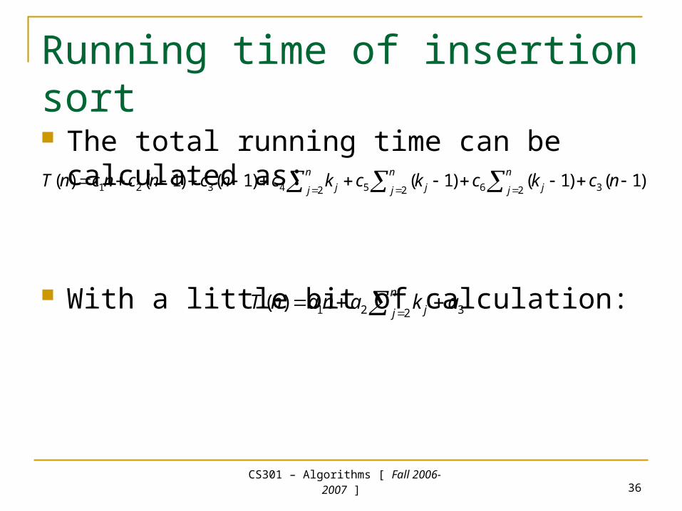
Running time of insertion sort The total running time can be calculated as:

With a little bit of calculation:

)1()1()1()1()1()( 3262524321 nckckckcncncncnT

n

j j

n

j j

n

j j

3221)( akananTn

j j


2007 ] 37

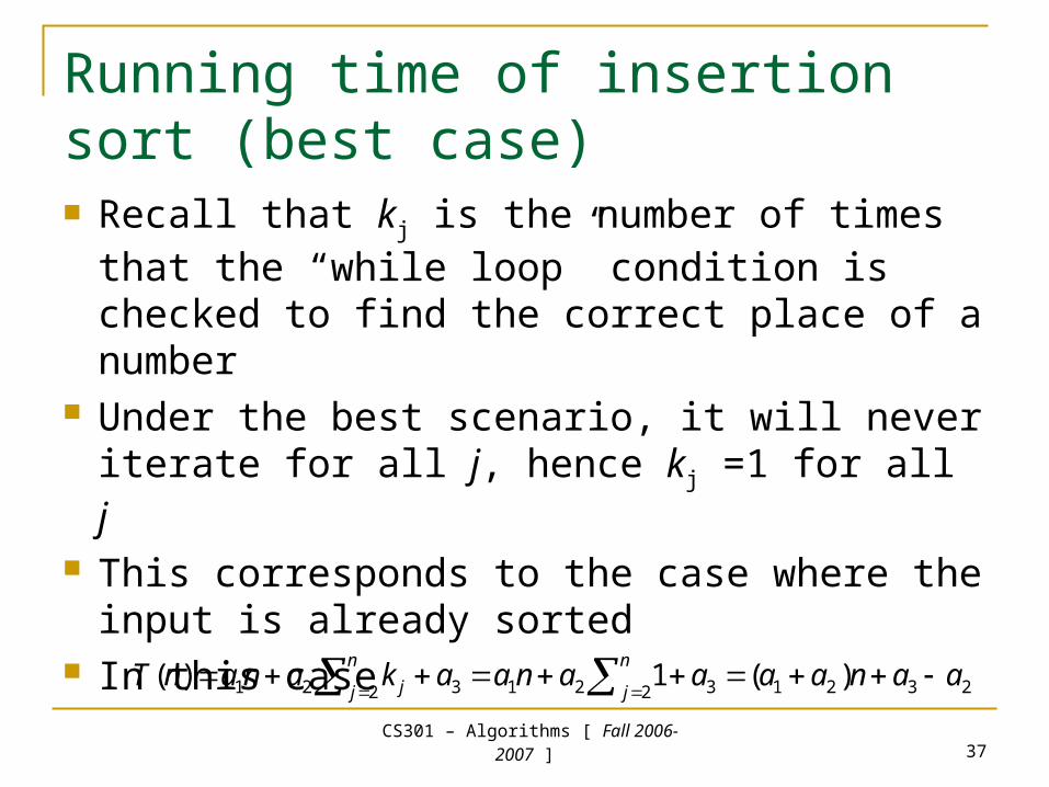
Running time of insertion sort (best case) Recall that kj is the number of times that the

“while loop” condition is checked to find the correct place of a number

Under the best scenario, it will never iterate for all j, hence kj =1 for all j

This corresponds to the case where the input is already sorted

In this case232132213221 )(1)( aanaaaanaakananT

n

j

n

j j


2007 ] 38

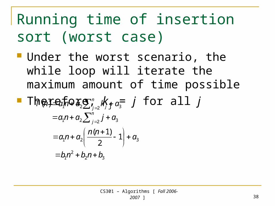
Running time of insertion sort (worst case) Under the worst scenario, the while loop will

iterate the maximum amount of time possible Therefore, kj = j for all j

3221)( akananTn

j j

3221 ajanan

j

321 12

)1(a

nnana

322

1 bnbnb


2007 ] 39

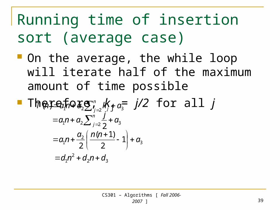
Running time of insertion sort (average case) On the average, the while loop will iterate half

of the maximum amount of time possible Therefore, kj = j/2 for all j

3221)( akananTn

j j

3221 2a

jana

n

j

32

1 12

)1(

2a

nnana

322

1 dndnd


2007 ] 40

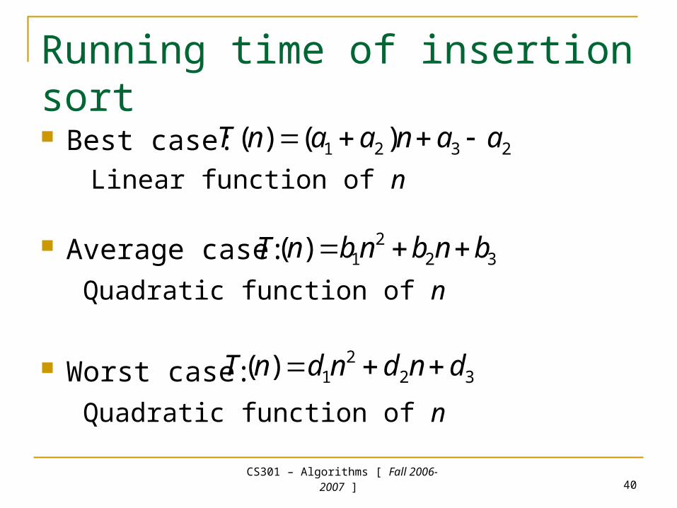
Running time of insertion sort Best case:

Linear function of n

Average case:

Quadratic function of n

Worst case:

Quadratic function of n

2321 )()( aanaanT

322

1)( bnbnbnT

322

1)( dndndnT


2007 ] 41

BREAK


2007 ] 42

Which running time we should use? In order to compare the running time of

algorithms, usually the “worst case running time” is used, because It gives an upper bound (it cannot go worse) Murphy’s law (most of the time, the worst case

appears) Average case is usually the same as the worst

case.


2007 ] 43

Asymptotic Analysis

Note that, in the running time analysis of the insertion sort algorithm, we ignored the actual cost of steps by abstracting them with constants : ci

We will go one step further, and show that these constants are not actually so important.


2007 ] 44

Asymptotic Analysis

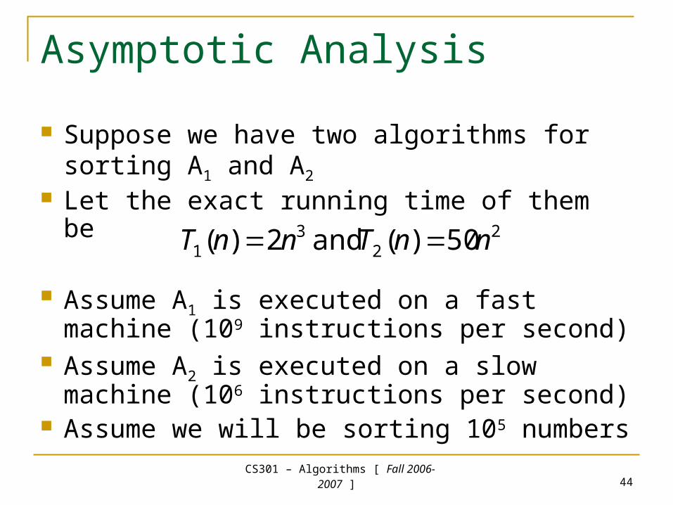
Suppose we have two algorithms for sorting A1 and A2

Let the exact running time of them be

Assume A1 is executed on a fast machine (109 instructions per second)

Assume A2 is executed on a slow machine (106 instructions per second)

Assume we will be sorting 105 numbers

22

31 50)( and 2)( nnTnnT


2007 ] 45

Asymptotic Analysis

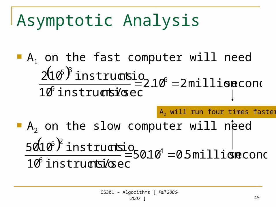
A1 on the fast computer will need

A2 on the slow computer will need

secondsmillion 210.2

ns/secinstructio 10

nsinstructio 102 69

35

secondsmillion 5.010.50

ns/secinstructio 10

nsinstructio 1050 46

25

A2 will run four times faster


2007 ] 46

Asymptotic Analysis

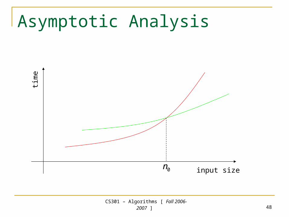
In real life, we will be interested in the performance of the algorithms on large inputs.

Therefore, even if the coefficients of the exact running time are small, it is the growth of the function (highest order term) that determines the performance of the algorithms as the input size gets bigger.


2007 ] 47

Asymptotic Analysis

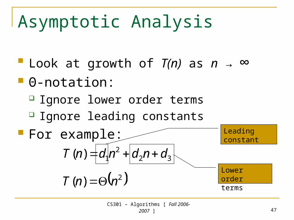
Look at growth of T(n) as n → ∞ Θ-notation:

Ignore lower order terms Ignore leading constants

For example:

322

1)( dndndnT

2)( nnT Lower order terms

Leading constant


2007 ] 48

Asymptotic Analysistim

e

input size0n


2007 ] 49

Algorithm Design Techniques

In general, there is no recipe for coming up with an algorithm for a given problem.

However, there are some algorithms design techniques that can be used to classify the algorithms.

Insertion sort uses so called “incremental approach”

Having sorted A[1..j-1], insert a new element A[j], forming a new, larger sorted sequence A[1..j]


2007 ] 50

Divide and Conquer

Another such design approach isDivide and Conquer

We will examine another algorithm for the sorting problem that follows divide and conquer approach

Divide and conquer algorithms are recursive in their nature.

It is relatively easy to analyze their running time


2007 ] 51

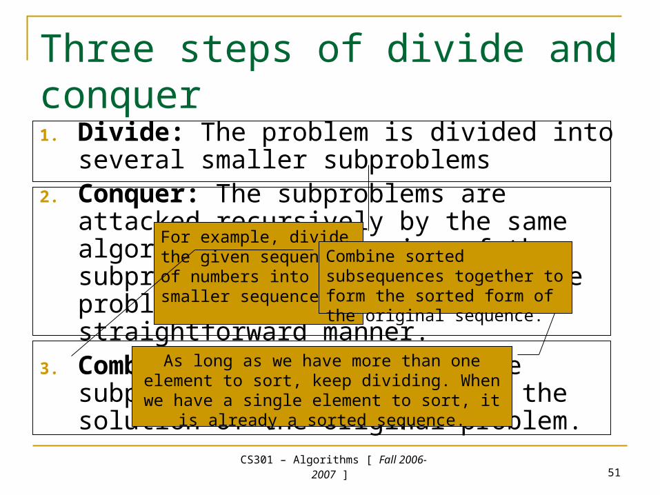
Three steps of divide and conquer1. Divide: The problem is divided into several

smaller subproblems2. Conquer: The subproblems are attacked

recursively by the same algorithm. When the size of the subproblem gets small enough, the problem is solved in a straightforward manner.

3. Combine: The solutions to the subproblems combined to form the solution of the original problem.

For example, divide the given sequence of numbers into smaller sequences.

As long as we have more than one element to sort, keep dividing. When we have a single

element to sort, it is already a sorted sequence.

Combine sorted subsequences together to form the sorted form of the original sequence.


2007 ] 52

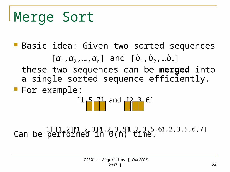
Merge Sort

Basic idea: Given two sorted sequences

[a1,a2,…,an] and [b1,b2,…bm]these two sequences can be merged into a single sorted sequence efficiently.

For example:[1,5,7] and [2,3,6]

Can be performed in Θ(n) time.

[1,2] [1,2,3,5,6,7][1,2,3,5,6][1,2,3,5][1,2,3][1]


2007 ] 53

Divide and conquer structure of the merge sort1. Divide: Divide the n-element sequence to be

sorted into two subsequences of n/2 elements each.

2. Conquer: Sort the subsequences recursively using merge sort (note that the recursion will bottom out when we have single element lists).

3. Combine: Merge the sorted subsequences using the merge operation explained before.


2007 ] 54

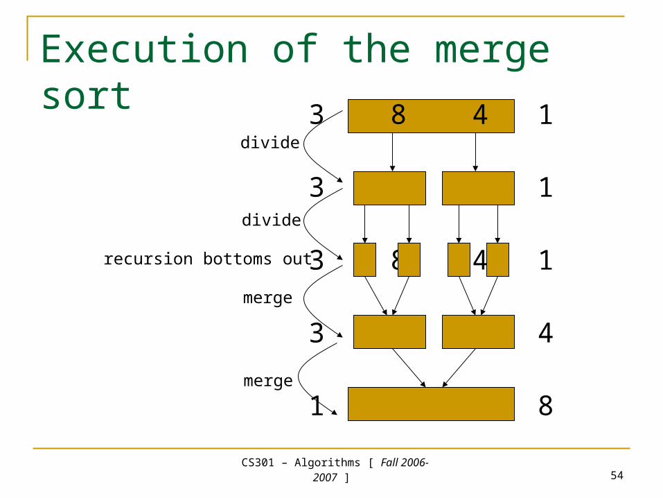
Execution of the merge sort

3 8 4 1

3 8 4 1

3 8 4 1

3 8 1 4

1 3 4 8

divide

divide

merge

merge

recursion bottoms out


2007 ] 55

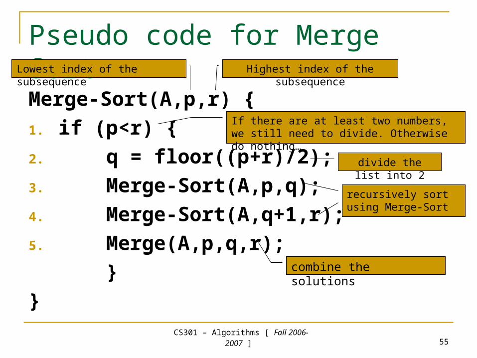
Pseudo code for Merge Sort

Merge-Sort(A,p,r) {

1. if (p<r) {

2. q = floor((p+r)/2);

3. Merge-Sort(A,p,q);

4. Merge-Sort(A,q+1,r);

5. Merge(A,p,q,r);

}

}

Lowest index of the subsequence Highest index of the subsequence

If there are at least two numbers, we still need to divide. Otherwise do nothing…

divide the list into 2

recursively sort using Merge-Sort

combine the solutions


2007 ] 56

Analysis of Divide and Conquer Algorithms If an algorithm is recursive, its running time

can often be described by a recurrence equation or recurrence.

A recurrence is a function that is defined recursively.


2007 ] 57

Analysis of Divide and Conquer Algorithms A recurrence for running time T(n) of a divide and

conquer algorithm is based on the three steps of the design approach: Suppose at each step the problem of size n is divided into

a subproblems each with a size n/b. Furthermore suppose dividing takes D(n) time.

When the problem size is small enough (say smaller than a constant c), we will apply a straightforward technique to solve the problem in constant amount of time, denoted by Θ(1).

Suppose combining the solutions takes C(n) time.


2007 ] 58

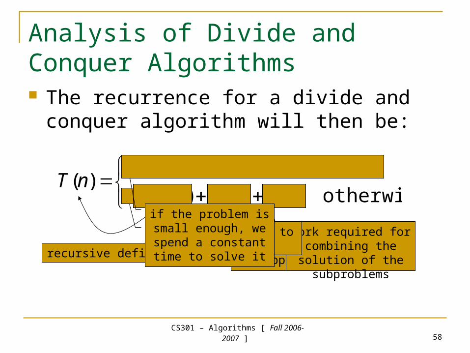
Analysis of Divide and Conquer Algorithms The recurrence for a divide and conquer

algorithm will then be:

otherwise)()()/(

if)1()(

nCnDbnaT

cnnT

recursive definition of the function

number of subproblems

size of each subproblem

work required for dividing into subproblems

work required for combining the solution

of the subproblems

time required to solve each subproblem

if the problem is small enough, we spend a

constant time to solve it


2007 ] 59

Analysis of Merge Sort

Note that the pseudo code for Merge-Sort works correctly when the number of elements are not even.

However, we will assume that the number of elements is a power of 2 for the analysis purposes.

We will later see that, this assumption does not actually make a difference.


2007 ] 60


Divide: The divide step just computes the middle of the array, hence it takes a constant amount of time → D(n) = Θ(1)

Conquer: Need to solve recursively two subproblems, each of which has size n/2. Hence this step takes 2T(n/2) time.

Combine: As we have seen earlier, merging two sorted sequences with n elements takes linear time → C(n) = Θ(n)


2007 ] 61


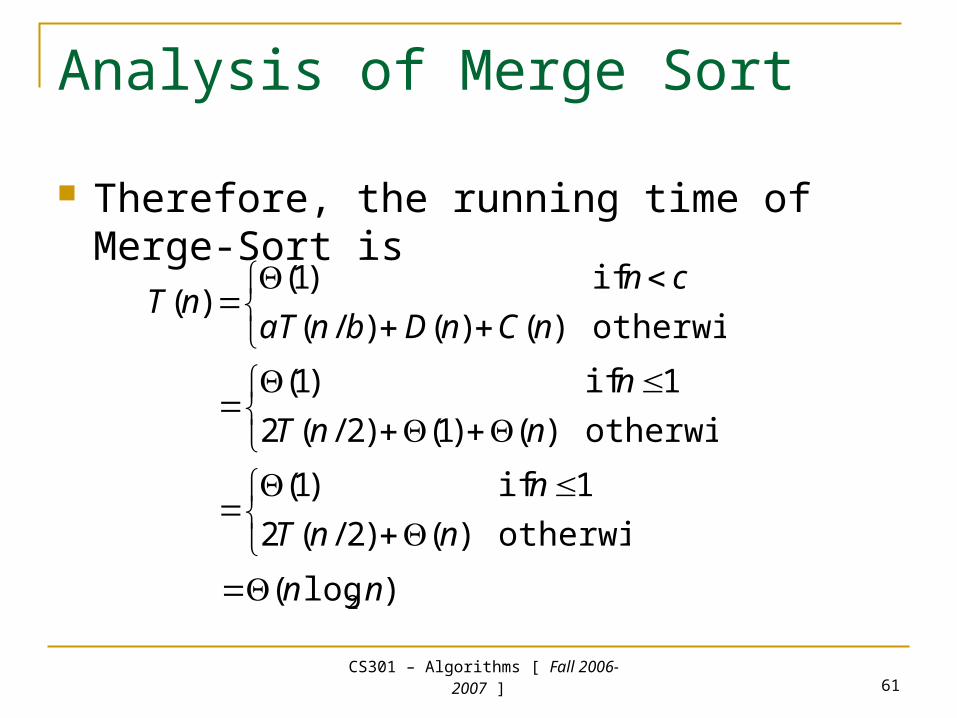
Therefore, the running time of Merge-Sort is

otherwise)()()/(

if)1()(

nCnDbnaT

cnnT

otherwise)()1()2/(2

1 if)1(

nnT

n

)log( 2 nn

otherwise)()2/(2

1 if)1(

nnT

n


2007 ] 62

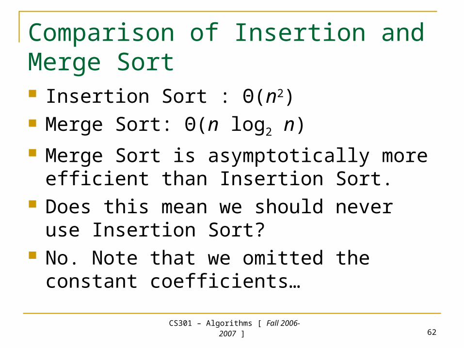
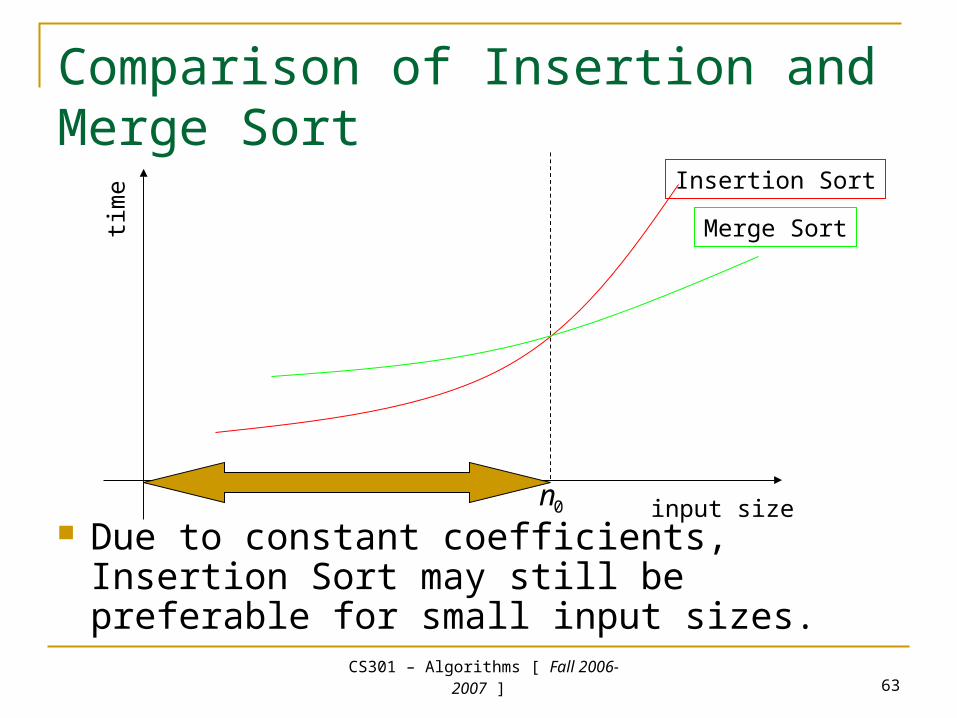
Comparison of Insertion and Merge Sort Insertion Sort : Θ(n2) Merge Sort: Θ(n log2 n) Merge Sort is asymptotically more efficient

than Insertion Sort. Does this mean we should never use

Insertion Sort? No. Note that we omitted the constant

coefficients…


2007 ] 63

Comparison of Insertion and Merge Sort

Due to constant coefficients, Insertion Sort may still be preferable for small input sizes.

time

input size0n

Insertion Sort

Merge Sort


2007 ] 64

GROWTH OF FUNCTIONS


2007 ] 65

Growth of Functions

The order of growth of running time provides a simple characterization of an algorithm’s efficiency a tool to compare the relative performances of algorithms

The exact running times can sometimes be derived, however, its use is limited, and not worth the effort for computing it, as when the inputs get large, the lower order terms and the constant coefficients are all dominated by the highest order term.

Usually, an algorithm that is asymptotically more efficient will be a better choice for all but very small input sizes.

We will introduce the asymptotic notations formally…


2007 ] 66

Asymptotic Notation

We will define the asymptotic running time of algorithms using a function T(n) whose domain is the set of natural numbers N={0,1,2,…}.

Although the notation will be introduced for only integer input sizes, sometimes it will be abused to apply to rational input sizes.

Other abuses of the notations will also be performed. Therefore, it is quite important to understand the formal definitions, to prevent the misuses due to abuses.


2007 ] 67

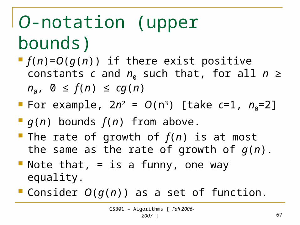
O-notation (upper bounds)

f(n)=O(g(n)) if there exist positive constants c and n0 such that, for all n ≥ n0, 0 ≤ f(n) ≤ cg(n)

For example, 2n2 = O(n3) [take c=1, n0=2] g(n) bounds f(n) from above. The rate of growth of f(n) is at most the same

as the rate of growth of g(n). Note that, = is a funny, one way equality. Consider O(g(n)) as a set of function.


2007 ] 68

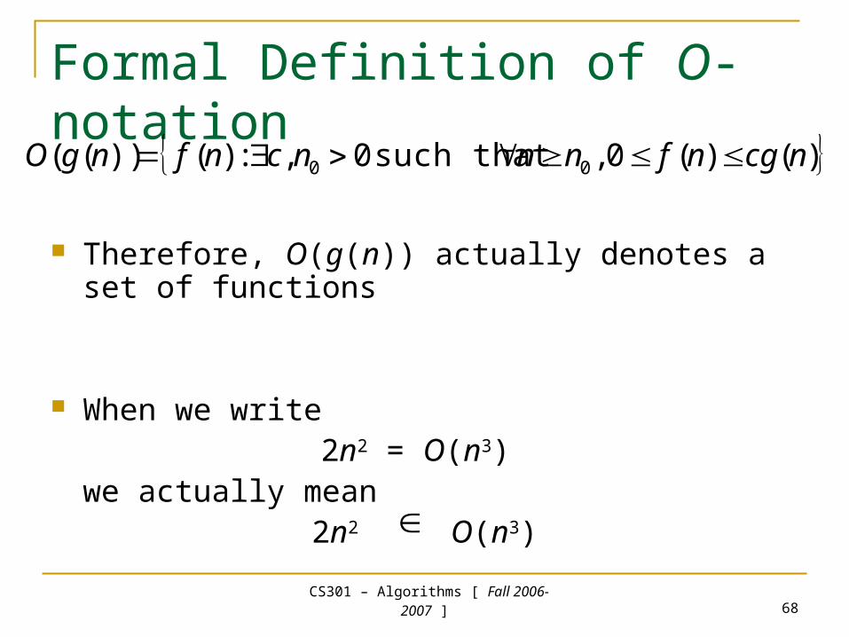
Formal Definition of O-notation

Therefore, O(g(n)) actually denotes a set of functions

When we write 2n2 = O(n3)

we actually mean 2n2 O(n3)

)()(0 ,such that 0,:)())(( 00 ncgnfnnncnfngO


2007 ] 69

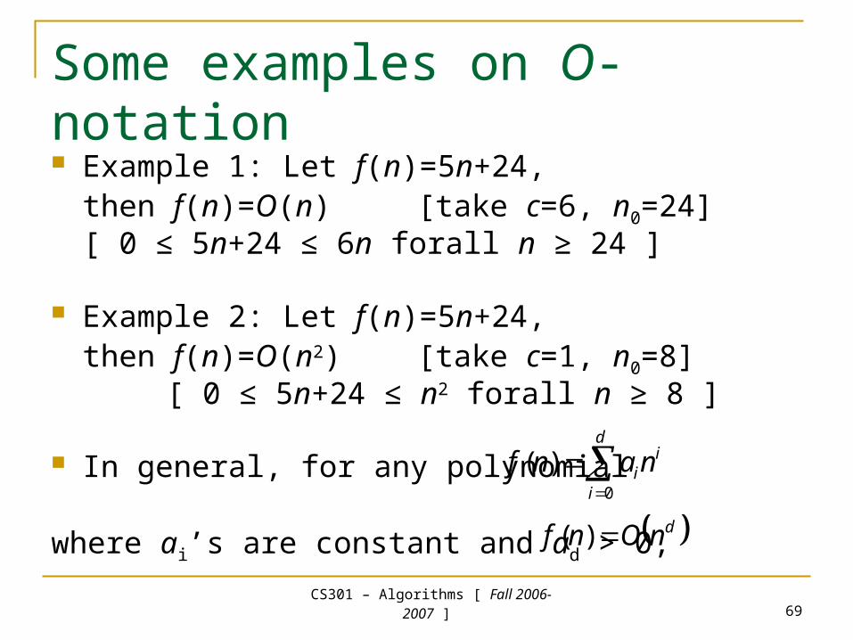
Some examples on O-notation Example 1: Let f(n)=5n+24,

then f(n)=O(n) [take c=6, n0=24][ 0 ≤ 5n+24 ≤ 6n forall n ≥ 24 ]

Example 2: Let f(n)=5n+24,then f(n)=O(n2) [take c=1, n0=8]

[ 0 ≤ 5n+24 ≤ n2 forall n ≥ 8 ]

In general, for any polynomial

where ai’s are constant and ad > 0,

d

i

iinanf

0

)(

dnOnf )(


2007 ] 70

O-notation in expressions

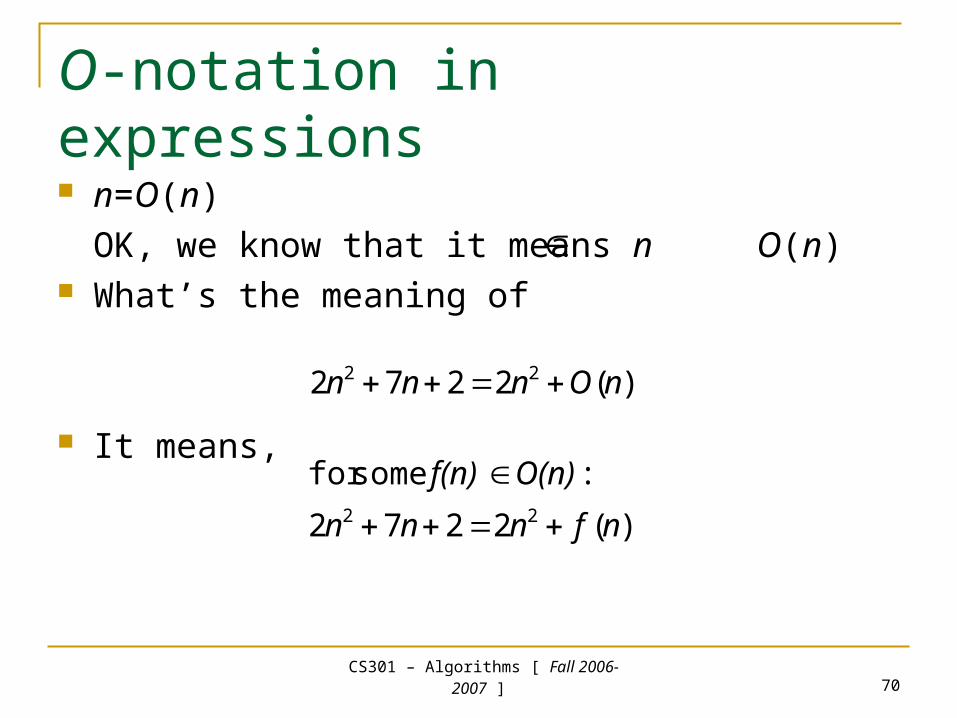
n=O(n)

OK, we know that it means n O(n) What’s the meaning of

It means,

)(2272 22 nOnnn

)(2272

: somefor 22 nfnnn

O(n)f(n)


2007 ] 71

O-notation in expressions

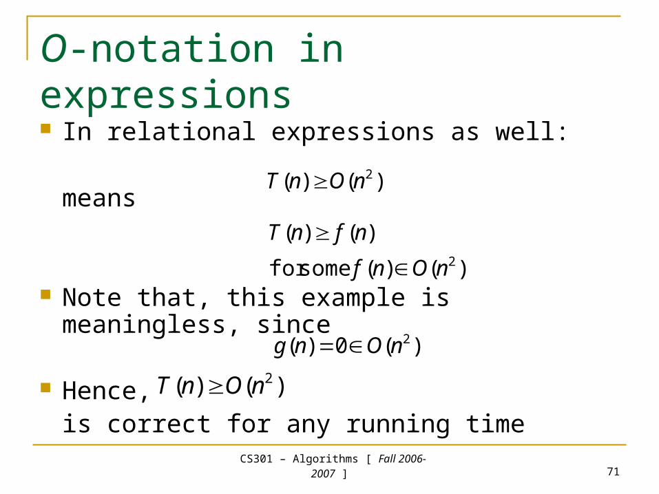
In relational expressions as well:

means

Note that, this example is meaningless, since

Hence, is correct for any running time

)()( 2nOnT

)()( somefor

)()(2nOnf

nfnT

)(0)( 2nOng

)()( 2nOnT


2007 ] 72

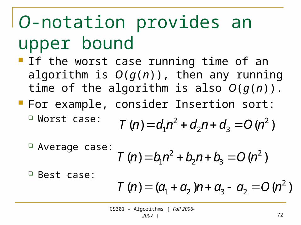
O-notation provides an upper bound If the worst case running time of an algorithm

is O(g(n)), then any running time of the algorithm is also O(g(n)).

For example, consider Insertion sort: Worst case:

Average case:

Best case:

)()( 232

21 nOdndndnT

)()( 232

21 nObnbnbnT

)()()( 22321 nOaanaanT


2007 ] 73

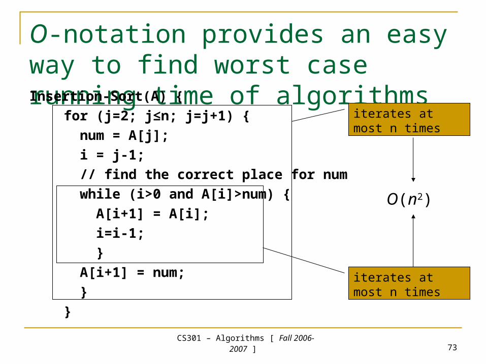
O-notation provides an easy way to find worst case running time of algorithmsInsertion-Sort(A) {

for (j=2; j≤n; j=j+1) {

num = A[j];

i = j-1;

// find the correct place for num

while (i>0 and A[i]>num) {

A[i+1] = A[i];

i=i-1;

}

A[i+1] = num;

}

}

iterates at most n times

iterates at most n times

O(n2)


2007 ] 74

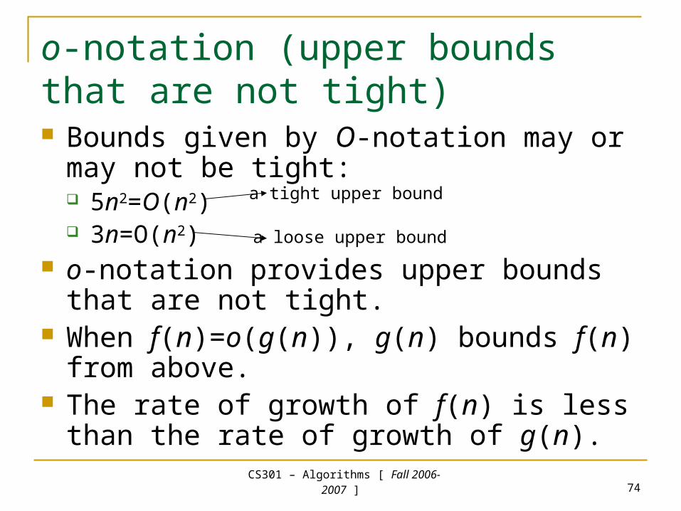
o-notation (upper bounds that are not tight) Bounds given by O-notation may or may not

be tight: 5n2=O(n2) 3n=O(n2)

o-notation provides upper bounds that are not tight.

When f(n)=o(g(n)), g(n) bounds f(n) from above.

The rate of growth of f(n) is less than the rate of growth of g(n).

a tight upper bound

a loose upper bound


2007 ] 75

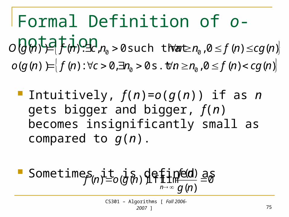
Formal Definition of o-notation

Intuitively, f(n)=o(g(n)) if as n gets bigger and bigger, f(n) becomes insignificantly small as compared to g(n).

Sometimes it is defined as

)()(0 ,such that 0,:)())(( 00 ncgnfnnncnfngO

)()(0 , s.t. 0,0:)())(( 00 ncgnfnnncnfngo

0)(

)(lim iff ))(()(

ng

nfngonf

n


2007 ] 76

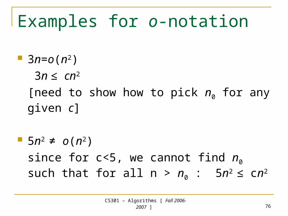
Examples for o-notation

3n=o(n2)

3n ≤ cn2

[need to show how to pick n0 for any given c]

5n2 ≠ o(n2)

since for c<5, we cannot find n0 such that for all n > n0 : 5n2 ≤ cn2


2007 ] 77

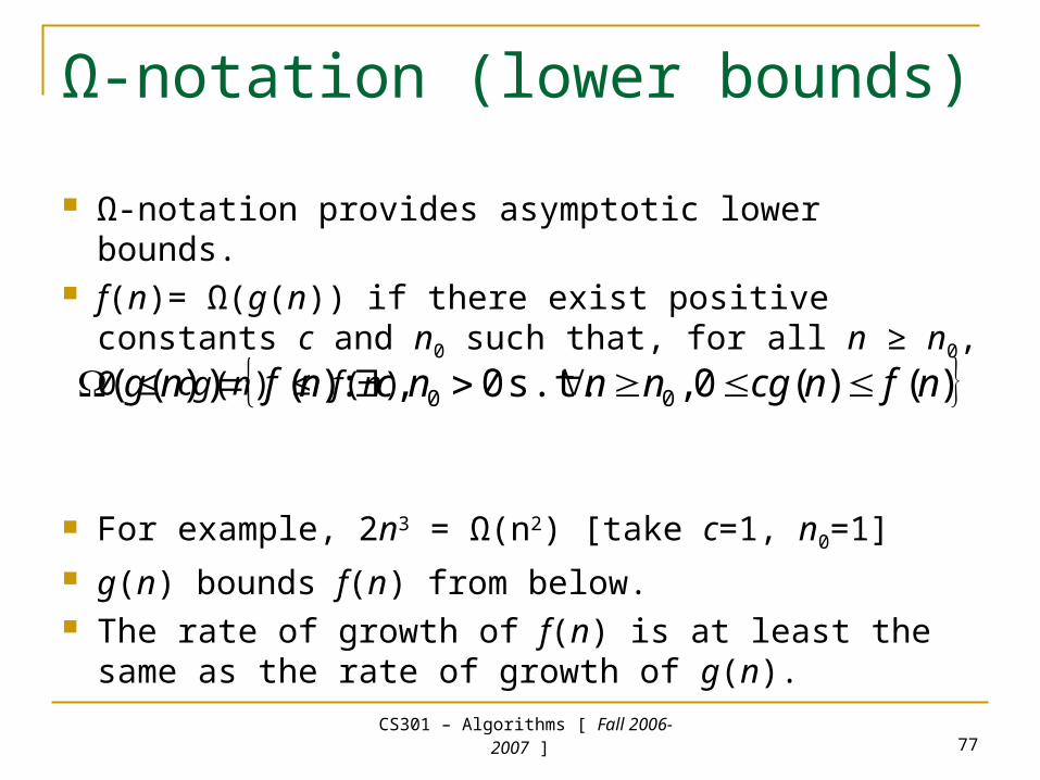
Ω-notation (lower bounds)

Ω-notation provides asymptotic lower bounds. f(n)= Ω(g(n)) if there exist positive constants c and

n0 such that, for all n ≥ n0, 0 ≤ cg(n) ≤ f(n)

For example, 2n3 = Ω(n2) [take c=1, n0=1] g(n) bounds f(n) from below. The rate of growth of f(n) is at least the same as the

rate of growth of g(n).

)()(0 , s.t. 0,:)())(( 00 nfncgnnncnfng


2007 ] 78

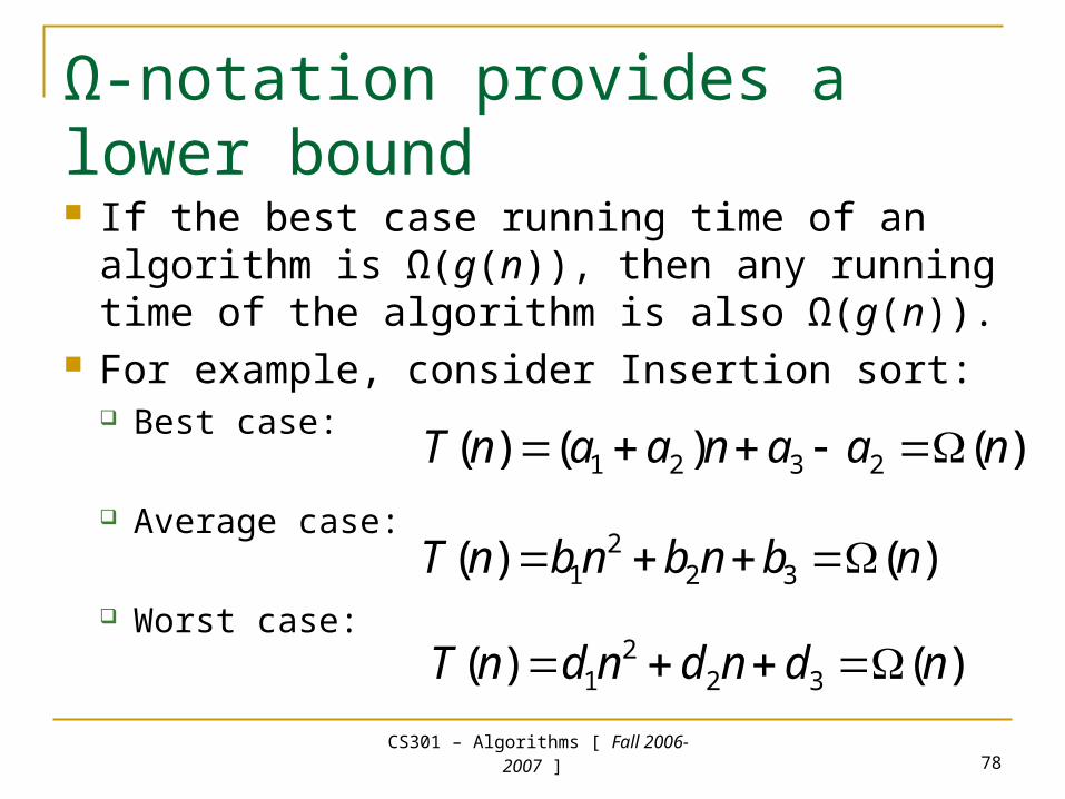
Ω-notation provides a lower bound If the best case running time of an algorithm

is Ω(g(n)), then any running time of the algorithm is also Ω(g(n)).

For example, consider Insertion sort: Best case:

Average case:

Worst case: )()( 322

1 ndndndnT

)()( 322

1 nbnbnbnT

)()()( 2321 naanaanT


2007 ] 79

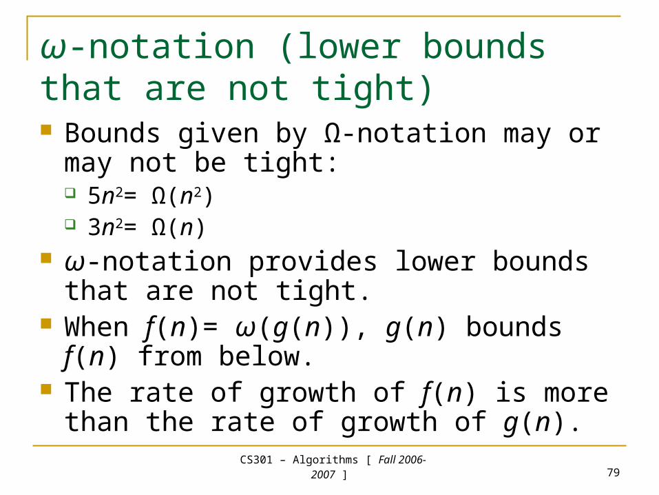
ω-notation (lower bounds that are not tight) Bounds given by Ω-notation may or may not

be tight: 5n2= Ω(n2) 3n2= Ω(n)

ω-notation provides lower bounds that are not tight.

When f(n)= ω(g(n)), g(n) bounds f(n) from below.

The rate of growth of f(n) is more than the rate of growth of g(n).


2007 ] 80

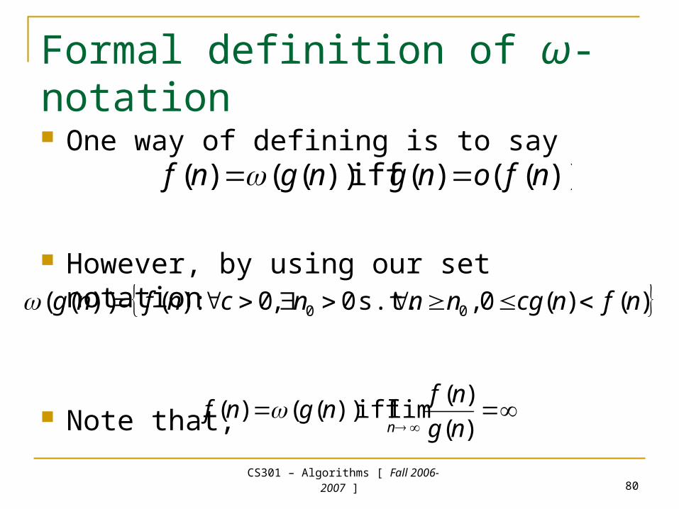
Formal definition of ω-notation One way of defining is to say

However, by using our set notation

Note that,

))(()( iff ))(()( nfongngnf

)()(0 , s.t. 0,0:)())(( 00 nfncgnnncnfng

)(

)(lim iff ))(()(

ng

nfngnf

n


2007 ] 81

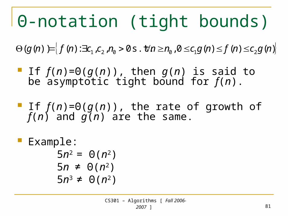
Θ-notation (tight bounds)

If f(n)=Θ(g(n)), then g(n) is said to be asymptotic tight bound for f(n).

If f(n)=Θ(g(n)), the rate of growth of f(n) and g(n) are the same.

Example: 5n2 = Θ(n2)5n ≠ Θ(n2)5n3 ≠ Θ(n2)

)()()(0 , s.t. 0,,:)())(( 210021 ngcnfngcnnnccnfng


2007 ] 82

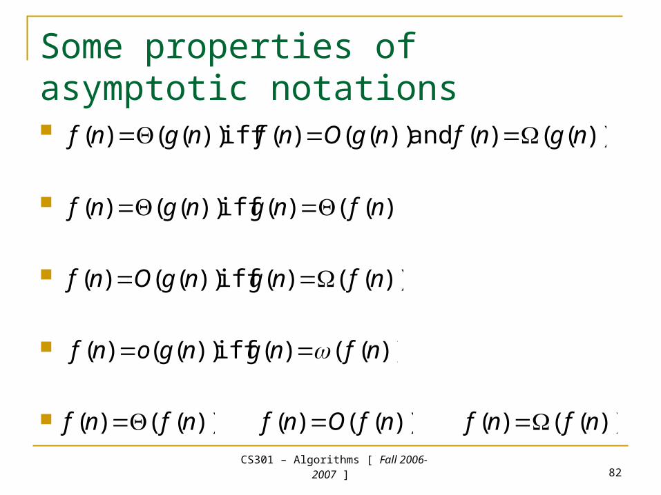
Some properties of asymptotic notations

))(()( and ))(()( iff ))(()( ngnfngOnfngnf

))(()( iff ))(()( nfngngnf

))(()( iff ))(()( nfngngOnf

))(()( iff ))(()( nfngngonf

))(()( nfnf ))(()( nfOnf ))(()( nfnf


2007 ] 83

Some more …

and this still holds when Θ above is replaced by any other asymptotic notation we have introduced (O,Ω,o,ω).

))(()( implies ))(()( and ))(()( nhnfnhngngnf


2007 ] 84

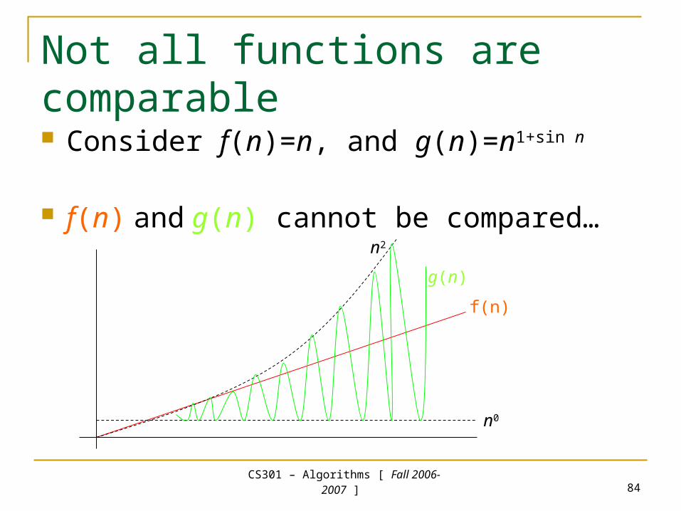
Not all functions are comparable Consider f(n)=n, and g(n)=n1+sin n

f(n) and g(n) cannot be compared…

f(n)

g(n)

n0

n2


2007 ] 85

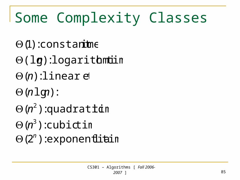
Some Complexity Classes

imeconstant t :)1( timeclogarithmi :)(lg n

elinear tim :)(n :)lg( nn

timequadratic :)( 2n timecubic :)( 3n

timelexponentia :)2( n

Documents

CS301 - Algorithms