CS235102 CS235102 Data StructuresData Structures

Chapter 10 Search StructuresChapter 10 Search Structures(Selected Topics)(Selected Topics)

Search Structures: OutlineSearch Structures: Outline

Optimal Binary Search TreesOptimal Binary Search Trees AVL TreesAVL Trees

Optimal binary search trees (1/14)Optimal binary search trees (1/14)

In this section we look at the construction of In this section we look at the construction of binary search trees for a static set of identifiersbinary search trees for a static set of identifiers Make no additions to or deletions from the identifiersMake no additions to or deletions from the identifiers Only perform searchesOnly perform searches

We examine the correspondence between a We examine the correspondence between a binary search tree and the binary search binary search tree and the binary search functionfunction

Optimal binary search trees (2/14)Optimal binary search trees (2/14) Examine:Examine: A binary search on the list A binary search on the list ( (do, if , whiledo, if , while) )

is equivalent to is equivalent to using the function using the function ((searchsearch2) on the 2) on the binary search treebinary search tree

Optimal binary search trees (3/14)Optimal binary search trees (3/14)

For a given static list, to decide a cost measure For a given static list, to decide a cost measure for search tree in order to find an optimal binary for search tree in order to find an optimal binary search treesearch tree Assume that we wish to search for an identifier at Assume that we wish to search for an identifier at

level level kk of a binary search tree. of a binary search tree. Generally, the number of iteration of binary search Generally, the number of iteration of binary search

equals the level number of the identifier we seek.equals the level number of the identifier we seek. It is reasonable to use the level number of a node as It is reasonable to use the level number of a node as

its cost.its cost.

A full binary tree may not be an optimal binary A full binary tree may not be an optimal binary search tree if the identifiers are search tree if the identifiers are searched for searched for with different frequencywith different frequency

Consider these Consider these two search trees, two search trees, If we search for If we search for each identifier with each identifier with equal probabilityequal probability In first tree, the average number of In first tree, the average number of

comparisons for successful search is 2.4.comparisons for successful search is 2.4. Comparisons for second tree is 2.2.Comparisons for second tree is 2.2.

The second tree hasThe second tree has a better worst case search time than a better worst case search time than

the first tree.the first tree. a better average behavior.a better average behavior.

1

1

22

22

3

33

4

(1+2+2+3+4)/5 = 2.4

(1+2+2+3+3)/5 = 2.2

Optimal binary Optimal binary search trees (5/14)search trees (5/14)

In evaluating binary search trees, In evaluating binary search trees, it is useful to add a special it is useful to add a special square node at every place square node at every place there is a null linksthere is a null links.. We call these nodes We call these nodes external nodesexternal nodes.. We also refer to the external nodes We also refer to the external nodes

as as failurefailure nodes. nodes. The remaining nodes are The remaining nodes are

internal nodesinternal nodes.. A binary tree with external nodes A binary tree with external nodes

added is an added is an extended binary treeextended binary tree

Optimal binary search trees (6/14)Optimal binary search trees (6/14) External / internal path lengthExternal / internal path length

The sum of all external / internal nodes’ levels.The sum of all external / internal nodes’ levels. For exampleFor example

Internal path length, Internal path length, II, is:, is:II = 0 + 1 + 1 + 2 + 3 = 7 = 0 + 1 + 1 + 2 + 3 = 7

External path length, External path length, EE, is :, is :EE = 2 + 2 + 4 + 4 + 3 + 2 = 17 = 2 + 2 + 4 + 4 + 3 + 2 = 17

A binary tree with A binary tree with nn internal internal nodes are related by the formula nodes are related by the formula EE = = II + 2 + 2nn

0

1 1

2 2 2 2

3 3

4 4

Optimal binary search trees (7/14)Optimal binary search trees (7/14) The maximum and minimum possible values for The maximum and minimum possible values for II

with with nn internal nodes internal nodes Maximum:Maximum:

The worst case occurs when the tree is skewed, that The worst case occurs when the tree is skewed, that is, the tree has a depth of is, the tree has a depth of nn..

Minimum:Minimum: We must have as many internal nodes We must have as many internal nodes as close to the as close to the

root as possibleroot as possible in order to obtain trees with minimal in order to obtain trees with minimal II One tree with minimal internal path length is the One tree with minimal internal path length is the

complete binary treecomplete binary tree that the distance of node that the distance of node ii from from the root is the root is loglog22ii..

Optimal binary search trees (8/14)Optimal binary search trees (8/14) In the binary search tree:In the binary search tree:

The identifiers The identifiers aa11, , aa22, …, , …, aann with with aa11 < < aa22 < … < < … < aann

The The probability of searching for each probability of searching for each aaii is is ppii

The total cost (when only successful searches are madThe total cost (when only successful searches are made) is:e) is:

If we replace the null subtree by a failure node, wIf we replace the null subtree by a failure node, we may partition the identifiers that are not in the bie may partition the identifiers that are not in the binary search tree into nary search tree into nn+1 classes +1 classes EEii, 0 , 0 ≤ ≤ i i ≤ ≤ nn EEii contains all identifiers contains all identifiers xx such that such that aaii < < xx < < aaii+1+1

For all identifiers in a particular class, For all identifiers in a particular class, EEii, the search ter, the search ter

minates at the same failure nodeminates at the same failure node

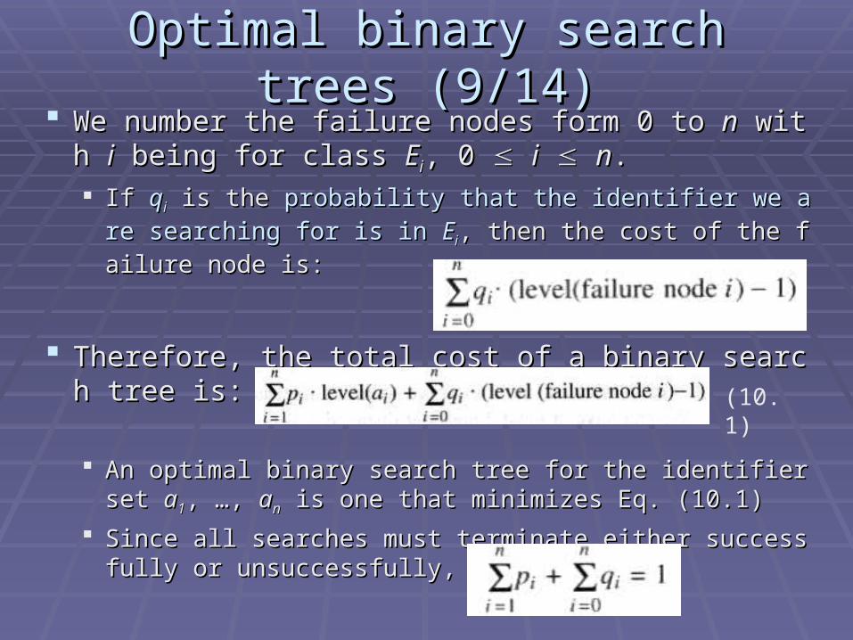
Optimal binary search trees (9/14)Optimal binary search trees (9/14) We number the failure nodes form 0 to We number the failure nodes form 0 to nn with with ii bei bei

ng for class ng for class EEii, 0 , 0 ii nn.. If If qqii is the is the probability that the identifier we are searching probability that the identifier we are searching

for is in for is in EEii, then the cost of the failure node is:, then the cost of the failure node is:

Therefore, the total cost of a binary search tree is:Therefore, the total cost of a binary search tree is:

An optimal binary search tree for the identifier set An optimal binary search tree for the identifier set aa11, …, , …,

aann is one that minimizes Eq. (10.1) is one that minimizes Eq. (10.1)

Since all searches must terminate either successfully or Since all searches must terminate either successfully or unsuccessfully, we haveunsuccessfully, we have

(10.1)

Optimal binary search trees (10/14)Optimal binary search trees (10/14) The possible binary search trees for the The possible binary search trees for the

identifier set (identifier set (aa11, , aa22, , aa33) = () = (dodo, , ifif, , whilewhile)) The identifiers with equal probabilities, The identifiers with equal probabilities,

ppii==aajj=1/7 for all =1/7 for all ii, , jj,, cost(tree cost(tree aa) = 15/7; ) = 15/7; cost(tree cost(tree bb) = 13/7 (optimal); ) = 13/7 (optimal);

cost(tree cost(tree cc) = 15/7; cost(tree ) = 15/7; cost(tree dd) = 15/7; ) = 15/7; cost(tree cost(tree ee) = 15/7;) = 15/7;

pp11 = 0.5, = 0.5, pp22 = 0.1, = 0.1, pp33 = 0.05, = 0.05,

qq00 = 0.15, = 0.15, qq11= 0.1, = 0.1, qq22 = 0.05, = 0.05, qq33 = 0.05 = 0.05 cost(tree cost(tree aa) = 2.65; ) = 2.65;

cost(tree cost(tree bb) = 1.9; ) = 1.9; cost(tree cost(tree cc) = 1.5; ) = 1.5; (optimal) (optimal) cost(tree cost(tree dd) = 2.05; ) = 2.05; cost(tree cost(tree ee) = 1.6;) = 1.6;

1

3 2

3 3

12

E0 E1

E2

E3

Optimal binary search trees (11/14)Optimal binary search trees (11/14) How do we determine the optimal binary search trHow do we determine the optimal binary search tr

ee for a given set of identifiers?ee for a given set of identifiers? We can make some observations about the properties oWe can make some observations about the properties o

f optimal binary search treesf optimal binary search trees TTijij : an: an optimal binary search tree for optimal binary search tree for aai+1i+1, …, , …, aajj, , i i << j j..

TTiiii is an empty tree for 0 is an empty tree for 0 ii nn and and TTijij is not defined for is not defined for ii > > jj..

ccijij : the : the cost of the search tree cost of the search tree TTijij.. By definition By definition cciiii is 0. is 0.

rrijij : the : the root of root of TTijij

wwijij : the : the weight of weight of TTij ij ,, By definition, By definition, rriiii = 0 and = 0 and wwiiii = = qqii , 0 , 0 ii nn . .

TT0n0n is an optimal binary search for is an optimal binary search for aa11, …, , …, aann. Its cost is . Its cost is cc00

nn, its weight is , its weight is ww0n0n, and its root is , and its root is rr0n0n

j

ikkkiij pqqw

1

)(

Optimal binary search trees (12/14)Optimal binary search trees (12/14) If If TTijij is an optimal binary search tree for is an optimal binary search tree for aai+1i+1, …, , …, aajj and and

rrijij = = kk, then , then kk satisfies the inequality satisfies the inequality

ii < < kk jj.. T has two subtrees T has two subtrees LL and and RR..

LL is the left subtree and the identifiers is the left subtree and the identifiers aai+1i+1, …, , …, aak-1k-1

RR is the right subtree and the identifiers is the right subtree and the identifiers aak+1k+1, …, , …, aajj

The cost The cost ccijij of of TTijij is ( is (wwij ij = = ppkk + w + wii,,kk-1 -1 + w+ wkjkj))

ppkk + + cost( cost(LL) + cost() + cost(RR) + weight() + weight(LL) + weight() + weight(RR) =) =

ppkk + + CCii,,kk-1 -1 + C+ Ckj kj ++ wwii,,kk-1 -1 + w+ wkj kj = = wwijij ++ CCii,,kk-1 -1 + C+ Ckj kj = =

wwijij ++

It shows us how to obtain It shows us how to obtain TT00nn and and CC00nn, starting from knowle, starting from knowle

dge that dge that TTiiii = = and and cciiii = 0 = 0

}{min 1, ljlijli

cc

ak

L R

Optimal binary search trees (13/14)Optimal binary search trees (13/14) ExampleExample

Let Let nn = 4, ( = 4, (aa11, , aa22, , aa33, , aa44) = () = (dodo, , forfor, , voidvoid, , whilewhile). ).

Let (Let (pp11, , pp22, , pp33, , pp44) = (3, 3, 1, 1) ) = (3, 3, 1, 1)

and (and (qq00, , qq11, , qq22, , qq33, , qq44) = (2, 3, 1, 1, 1).) = (2, 3, 1, 1, 1).

Initially Initially wwiiii = = qqii , , cciiii = 0, and = 0, and rrii ii = 0, 0 ≤ = 0, 0 ≤ ii ≤ 4 ≤ 4ww0101 = p= p11 + + w w0000 + w+ w1111 = p= p11 + q+ q11 + w+ w0000 = 8 = 8cc0101 = = w w0101 + min{ + min{cc0000 + +cc1111} = 8, } = 8, rr0101 = 1 = 1

ww1212 = = pp22 + + ww1111 + + ww2222 = = pp22 + +qq22 + +ww1111 = 7 = 7cc1212 = = ww1212 + min{ + min{cc1111 + +cc2222} = 7, } = 7, rr1212 = 2 = 2

ww2323 = = pp33 + + ww2222 + + ww3333 = = pp33 + +qq33 + +ww2222 = 3 = 3cc2323 = = ww2323 + min{ + min{cc2222 + +cc3333} = 3, } = 3, rr2323 = 3 = 3

ww3434 = = pp44 + + ww3333 + + ww4444 = = pp44 + +qq44 + +ww3333 = 3 = 3cc3434 = = ww3434 + min{ + min{cc3333 + +cc4444} = 3} = 3, r, r3434 = 4 = 4

Optimal binary search trees (14/14)Optimal binary search trees (14/14) wwiiii = = qqii

wwij ij = = ppkk + w + wii,,kk-1 -1 + w+ wkjkj

ccij ij = = wwijij ++ cciiii = 0 = 0 rriiii = 0 = 0 rrijij = = ll

Computation is carried out row-wise from row 0 to row 4

}{min 1, ljlijli

cc

The optimal search tree as the result

1

2

3

4

((aa1, 1, aa2, 2, aa3, 3, aa4) = (4) = (dodo,,forfor,,voidvoid,,whilewhile))

((pp1, 1, pp2, 2, pp3, 3, pp4) = (3, 3, 1, 1) 4) = (3, 3, 1, 1) ((qq0, 0, qq1, 1, qq2, 2, qq3, 3, qq4) = (2, 3, 1, 1, 1)4) = (2, 3, 1, 1, 1)

AVL Trees (1/17)AVL Trees (1/17) We also may maintain dynamic tables as binary We also may maintain dynamic tables as binary

search trees.search trees. Figure 10.8 shows the binary search tree obtained by Figure 10.8 shows the binary search tree obtained by

entering the months entering the months JanuaryJanuary to to DecemberDecember, in that order, , in that order, into an initially empty binary search treeinto an initially empty binary search tree

The maximum number of comparisons needed to search The maximum number of comparisons needed to search for any identifier in the tree of Figure 10.8 is six for any identifier in the tree of Figure 10.8 is six (for (for NovemberNovember).).

Average number of Average number of comparisons is comparisons is 42/12 = 3.542/12 = 3.5

AVL Trees (2/17)AVL Trees (2/17) Suppose that we now enter the months into an Suppose that we now enter the months into an

initially empty tree in initially empty tree in alphabetical orderalphabetical order The tree degenerates into the chainThe tree degenerates into the chain number of comparisons: number of comparisons:

maximum: 12, and average: 6.5maximum: 12, and average: 6.5 in the worst in the worst

case, binary case, binary search trees search trees correspond to correspond to sequential sequential searching in an searching in an ordered listordered list

Another insert sequenceAnother insert sequence In the order In the order JulJul, , FebFeb, , MayMay, , AugAug, , JanJan, , MarMar, , OctOct, , AprApr, , DecDec, , JJ

unun, , NovNov, and , and SepSep, by Figure 10.9., by Figure 10.9. Well balanced and does not have any paths to leaf nodes tWell balanced and does not have any paths to leaf nodes t

hat are much longer than others.hat are much longer than others. Number of comparisons: Number of comparisons:

maximum: 4, and average: 37/12 maximum: 4, and average: 37/12 3.1. 3.1. All intermediate trees created during the construction of All intermediate trees created during the construction of

Figure 10.9 are also well balancedFigure 10.9 are also well balanced If all permutations are equally probable, then we can prove If all permutations are equally probable, then we can prove

that the average that the average search and search and insertion time is insertion time is O(logO(lognn) for ) for nn nodenode binary binary search treesearch tree

AVL Trees (4/17)AVL Trees (4/17) Since we have a dynamic environment, it is hard to Since we have a dynamic environment, it is hard to

achieve:achieve: Required to add new elements and maintain a complete Required to add new elements and maintain a complete

binary tree without a significant increasing timebinary tree without a significant increasing time

Adelson-Velskii and Landis introduced a binary tree Adelson-Velskii and Landis introduced a binary tree structure (structure (AVL treesAVL trees):): Balanced with respect to the heights of the subtrees.Balanced with respect to the heights of the subtrees. We can perform dynamic retrievals in O(logWe can perform dynamic retrievals in O(lognn) time for a tr) time for a tr

ee with n nodes.ee with n nodes. We can enter an element into the tree, or delete an elemWe can enter an element into the tree, or delete an elem

ent form it, in O(logent form it, in O(lognn) time. The resulting tree remain heig) time. The resulting tree remain height balanced.ht balanced.

As with binary trees, we may define AVL tree recursivelyAs with binary trees, we may define AVL tree recursively

AVL Trees (5/17)AVL Trees (5/17) Definition:Definition:

An empty binary tree is height balanced. If An empty binary tree is height balanced. If TT is a nonemp is a nonempty binary tree with ty binary tree with TTLL and and TTRR as its left and right subtrees, as its left and right subtrees,

then then TT is is height balanced iffheight balanced iff TTLL and and TTRR are height balanced, and are height balanced, and

||hhLL - - hhRR| | 1 where 1 where hhLL and and hhRR are the heights of are the heights of TTLL and and TTRR, respec, respec

tively.tively.

The definition of a height balanced binary tree requThe definition of a height balanced binary tree requires that ires that every subtree every subtree also be height also be height balancedbalanced

AVL Trees (6/17)AVL Trees (6/17) This time we will insert the months into the tree in the This time we will insert the months into the tree in the

orderorder MarMar, , MayMay, , NovNov, , AugAug, , AprApr, , JanJan, , DecDec, , JulJul, , FebFeb, , JunJun, , OctOct, , SepSep

It shows the tree as it grows, and the It shows the tree as it grows, and the restructuring invrestructuring involved in keeping it balancedolved in keeping it balanced..

The numbers by each node represent the difference iThe numbers by each node represent the difference in heights between the left and right subtrees of that nn heights between the left and right subtrees of that nodeode

We refer to this as the balance factor of the nodeWe refer to this as the balance factor of the node Definition:Definition:

The balance factor, The balance factor, BF(T)BF(T), of a node, , of a node, TT, in a binary tree is d, in a binary tree is defined as efined as hhLL - - hhRR, where , where hhLL((hhRR) are the heights of the left(rig) are the heights of the left(right) subtrees of ht) subtrees of TT..For any node For any node TT in an AVL tree in an AVL tree BF(T)BF(T) = -1, 0, or 1. = -1, 0, or 1.

AVL Trees (7/17)AVL Trees (7/17) Insertion into an AVL treeInsertion into an AVL tree

AVL Trees (8/17)AVL Trees (8/17) Insertion into an AVL tree (cont’d)Insertion into an AVL tree (cont’d)

Insertion into an AVL tree (cont’d)Insertion into an AVL tree (cont’d)

Insertion into an AVL tree (cont’d)Insertion into an AVL tree (cont’d)

AVL Trees (11/17)AVL Trees (11/17) We carried out the rebalancing using four different We carried out the rebalancing using four different

kinds of rotations: kinds of rotations: LLLL, , RRRR, , LRLR, and , and RLRL LLLL and and RRRR are symmetric as are are symmetric as are LRLR and and RLRL These rotations are characterized by the nearest ancestThese rotations are characterized by the nearest ancest

or, or, AA, of the inserted node, , of the inserted node, YY, , whose balance factor becwhose balance factor becomes omes 22.. LLLL: : YY is inserted in the left subtree of the left subtree of is inserted in the left subtree of the left subtree of AA.. LRLR: : YY is inserted in the right subtree of the left subtree of is inserted in the right subtree of the left subtree of AA RRRR: : YY is inserted in the right subtree of the right subtree of is inserted in the right subtree of the right subtree of AA RLRL: : YY is inserted in the left subtree of the right subtree of is inserted in the left subtree of the right subtree of AA

Rebalancing rotationsRebalancing rotationsAVL Trees (12/17)AVL Trees (12/17)

Rebalancing rotationsRebalancing rotationsAVL Trees (13/17)AVL Trees (13/17)

Rebalancing rotations (cont’d)Rebalancing rotations (cont’d)

AVL Trees (14/17)AVL Trees (14/17)

Rebalancing rotations (cont’d)Rebalancing rotations (cont’d)AVL Trees (15/17)AVL Trees (15/17)

Rebalancing rotations (cont’d)Rebalancing rotations (cont’d)

AVL Trees (17/17)AVL Trees (17/17) Complexity:Complexity:

In the case of binary search trees, if there were In the case of binary search trees, if there were nn nod nodes in the tree, then es in the tree, then hh (the height of tree) could be be (the height of tree) could be be nn and the worst case insertion time would be O(and the worst case insertion time would be O(nn).).

In the case of AVL trees, since In the case of AVL trees, since hh is at most (log is at most (log nn), th), the worst case insertion time is O(log e worst case insertion time is O(log nn). ).

Figure 10.13 compares the worst case times of certaiFigure 10.13 compares the worst case times of certain operationsn operations