CS137 – Introduction to ScientificComputing

Lecture 13 – More on InterpolationFelix Kwok

Stanford University

CS137/Lecture 13 – p. 1/26

High-Degree Polynomial Interpolation

Last time we showed that, for Lagrangian interpolation,

f(x) = pn(x) +∆n+1(x)

(n + 1)!f (n+1)(ξ),

where ∆n(x) =∏n+1

i=0 (x − xi). This does not mean thatpn(x) → f(x) as n → ∞ because

1. f (n+1)(ξ) may not be nicely bounded,

2. ∆n+1(x) can grow; in particular, the product can belarge near end points, since (x − xi) is large for most i

CS137/Lecture 13 – p. 2/26

Runge’s Example

f(x) =1

1 + 25x2, x ∈ [−1, 1]

Suppose we pick equally spaced nodes.

−1 −0.8 −0.6 −0.4 −0.2 0 0.2 0.4 0.6 0.8 1−0.5

0

0.5

1

1.5

2Runge’s Example

f(t) = 1/(1+25t2)p

5(t)

p10

(t)

CS137/Lecture 13 – p. 3/26

Runge’s Example

Highly oscillatory (Typical for high-degree polynomials)

Non-convergence near the end-points

Possible solutions:

1. Use more nodes near the end-points=⇒ Chebyshev Polynomials

2. Divide into subintervals, and use a different low-degreepolynomial for each subinterval=⇒ Splines

CS137/Lecture 13 – p. 4/26

Chebyshev Polynomials

Tn(x) =

{

cos(n cos−1(x)), |x| ≤ 1

(sgn(x))n cosh(n cosh−1(|x|)), |x| ≥ 1

Examples:

T0(x) = 1

T1(x) = x

T2(x) = cos(2 cos−1 x) = 2 cos2(cos−1 x) − 1 = 2x2 − 1

T3(x) = cos(3 cos−1 x) = 4 cos3(cos−1 x) − 3 cos(cos−1 x) =

4x3 − 3x

CS137/Lecture 13 – p. 5/26

Chebyshev Polynomials

In general,

cos(A) + cos(B) = 2 cos

(

A + B

2

)

cos

(

A − B

2

)

socos(n + 1)θ + cos(n − 1)θ = 2 cos nθ cos θ

impliesTn+1(x) = 2xTn(x) − Tn−1(x)

Note: Leading coefficient of Tn(x) is 2n−1.

CS137/Lecture 13 – p. 6/26

Properties of Tn(x)

1. |Tn(x)| ≤ 1 for |x| ≤ 1

2. Maximum modulus attained at tj = cos(jπ/n),j = 0, . . . , n:

Tn(tj) = (−1)j .

3. Tn(x) is a degree-n polynomial =⇒ n roots:

cos(nθ) = 0 =⇒ θj =(2j − 1)π

2n, j = 1, . . . , n

So Tn(xj) = 0, xj = cos(

(2j−1)π2n

)

, i.e. all n roots lie

within [−1, 1].

4. All roots are distinct =⇒ alternating signs.

CS137/Lecture 13 – p. 7/26

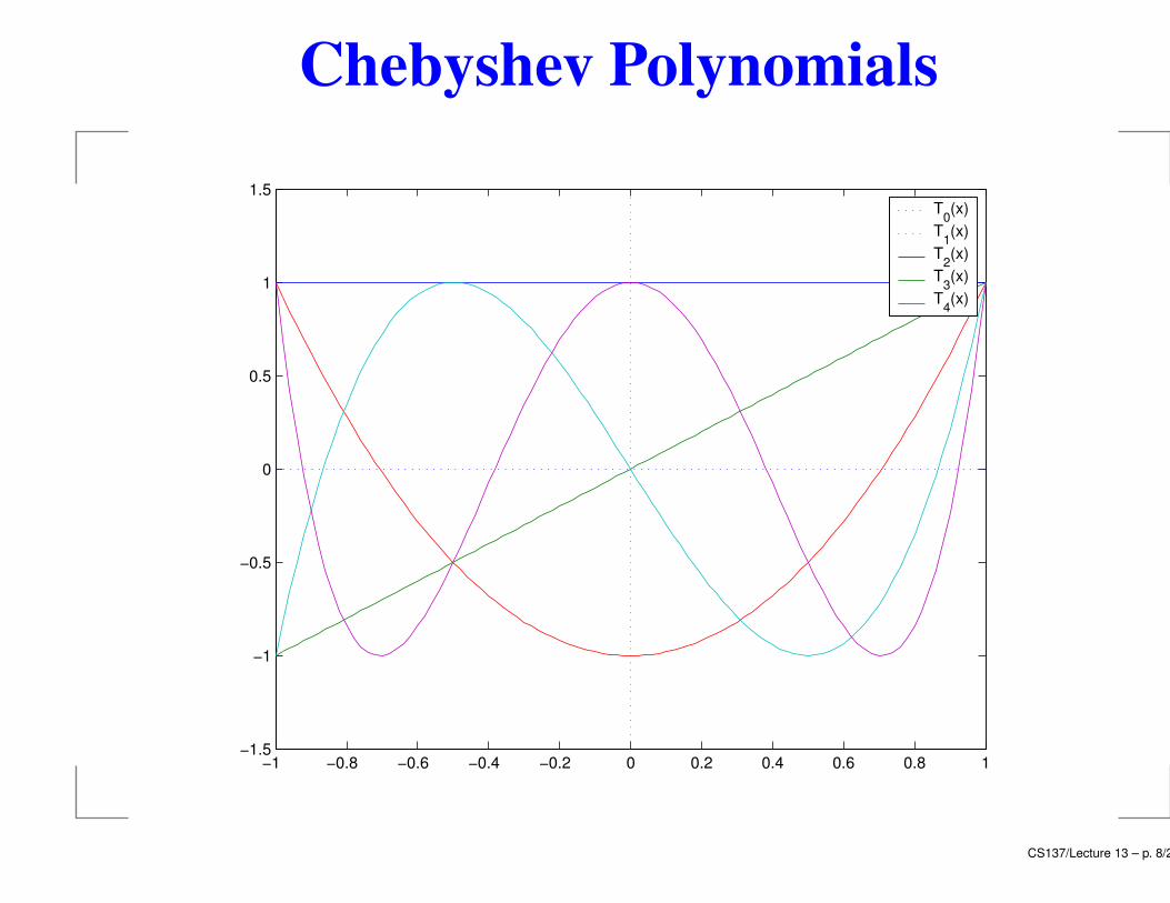
Chebyshev Polynomials

−1 −0.8 −0.6 −0.4 −0.2 0 0.2 0.4 0.6 0.8 1−1.5

−1

−0.5

0

0.5

1

1.5T

0(x)

T1(x)

T2(x)

T3(x)

T4(x)

CS137/Lecture 13 – p. 8/26

Unequally Spaced Nodes for Interpolation

Recall

f(x) = pn−1(x) +∆n(x)

n!f (n)(ξ).

Suppose we are allowed to evaluate f(x) at n differentpoints within the interval [−1, 1] for the purpose ofinterpolation, and we want to pick the nodes to minimize∆n(x).

Answer: Choose xj to be the zeros of Tn(x)! Then

∆̂n(x) = 2−n+1Tn(x)

(since ∆n is monic).

CS137/Lecture 13 – p. 9/26

Optimality of Tn(x)

Claim: Let Γn(x) = xn + · · · (monic polynomial). Then

max−1≤x≤1

|Γn(x)| ≥ max−1≤x≤1

|∆̂n(x)|.

Proof: Suppose, on the contrary, that

max−1≤x≤1

|Γn(x)| < max−1≤x≤1

|∆̂n(x)|.

Define D(x) = ∆̂n(x) − Γn(x). Then for tj = cos(jπ/n),j = 0, . . . , n, we have

|Γn(tj)| < max−1≤x≤1

|∆̂n(x)| = |∆̂n(tj)|.

CS137/Lecture 13 – p. 10/26

Optimality of Tn(x)

Thus, D(tj) has the same sign as ∆̂n(tj), i.e.

D(tj)

{

> 0 for j even,< 0 for j odd,

j = 0, . . . , n. There are n sign changes between t0 = 1 andtn = −1, so D(x) has at least n zeros. But since Γn(x) and∆̂n(x) are both monic, we have

D(x) = ∆̂n(x) − Γn(x)

= (xn + · · · ) − (xn + · · · ) = cxn−1 + · · ·

has degree at most n − 1 =⇒ Contradiction!

CS137/Lecture 13 – p. 11/26

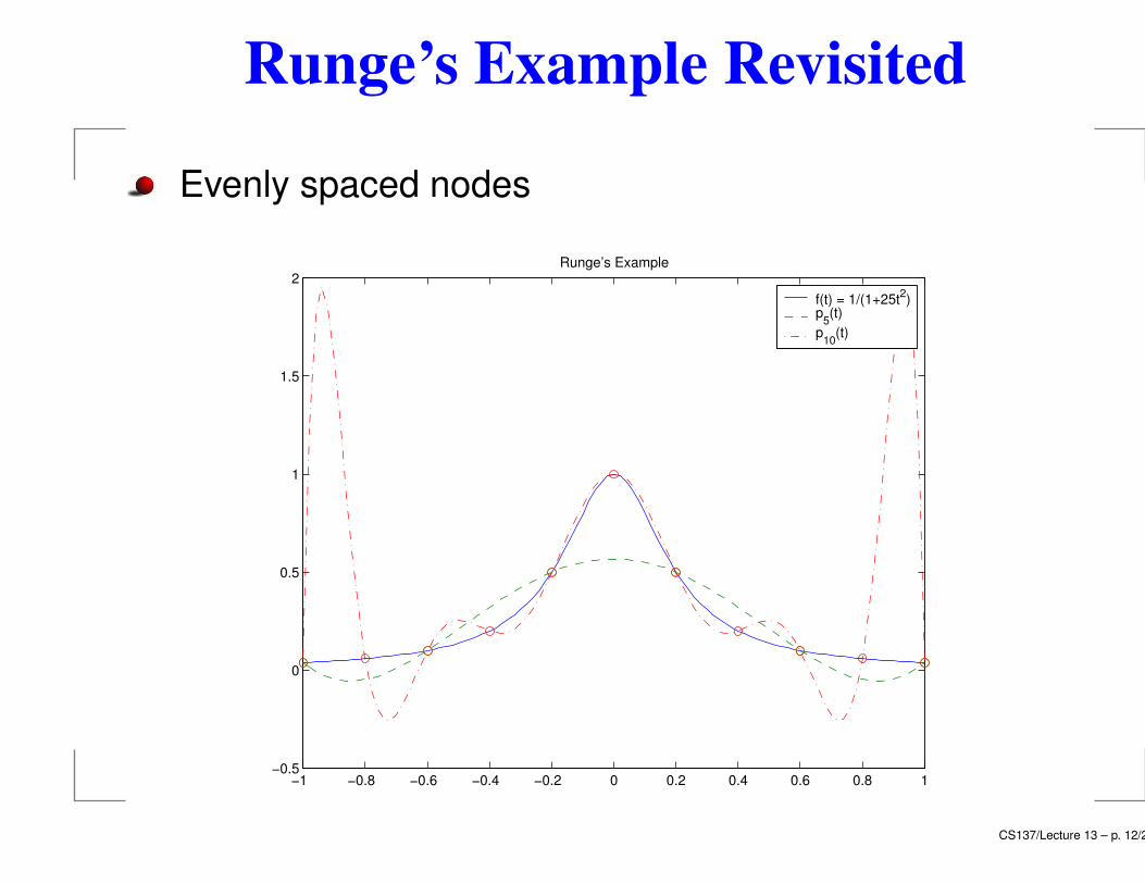
Runge’s Example Revisited

Evenly spaced nodes

−1 −0.8 −0.6 −0.4 −0.2 0 0.2 0.4 0.6 0.8 1−0.5

0

0.5

1

1.5

2Runge’s Example

f(t) = 1/(1+25t2)p

5(t)

p10

(t)

CS137/Lecture 13 – p. 12/26

Runge’s Example Revisited

Chebyshev nodes

−1 −0.8 −0.6 −0.4 −0.2 0 0.2 0.4 0.6 0.8 1−0.2

0

0.2

0.4

0.6

0.8

1

1.2Runge’s Example

f(t) = 1/(1+25t2)p

5(t)

p10

(t)

CS137/Lecture 13 – p. 13/26

Remarks on Chebyshev Interpolation

1. Can be proved to converge for sufficiently smoothunderlying functions

2. For intervals other than [−1, 1], use a change ofvariables:

x =(a + b) + (b − a)s

2,

This brings x ∈ [a, b] to s ∈ [−1, 1].

3. High-degree interpolating polynomials still contain“wiggles”, may be unphysical.

CS137/Lecture 13 – p. 14/26

Piecewise polynomial interpolation

Basic Idea: Instead of fitting all data with the samepolynomial, use different polynomials for each intervalIj = [xj−1, xj ].

Example: piecewise linear

0 0.5 1 1.5 2 2.5 3 3.5 4 4.5 50

2

4

6

8

10

12Linear interpolation

CS137/Lecture 13 – p. 15/26

Quadratic Splines

For high-order piecewise polynomials, require continuityof derivatives

Example: piecewise quadratics. Given x0 < · · · < xn

and y0, . . . , yn, we require

pj(x) = aj + bj(x − xj−1) + cj(x − xj−1)2

pj(xj−1) = yj−1

pj(xj) = yj

p′j(xj) = p′j+1(xj)

Number of unknowns: 3n

Number of constraints: n + n + (n − 1) = 3n − 1

Prescribe intial/final condition: p′1(x0) = y′0 or p′n(xn) = y′nCS137/Lecture 13 – p. 16/26

Quadratic Splines

Linear system: assuming hj = xj − xj−1,

pj(xj−1) = aj = yj−1

pj(xj) = aj + bjhj + cjh2j = yj

=⇒ bjhj + cjh2j = yj − yj−1

p′j(xj) = bj + 2cjhj

= bj+1 = p′j+1(xj)

p′1(x0) = y′0

Sparse matrix of size 2n − 1

Interpolant is continuously differentiable

Discontinuous second derivativesCS137/Lecture 13 – p. 17/26

Quadratic Splines

0 0.5 1 1.5 2 2.5 3 3.5 4 4.5 5−4

−2

0

2

4

6

8

10

12

14Quadratic spline, y’(0) = 0

CS137/Lecture 13 – p. 18/26

Cubic Splines

Formulation:

pj(x) = aj + bj(x − xj−1) + cj(x − xj−1)2 + dj(x − xj−1)

3

pj(xj−1) = yj−1

pj(xj) = yj

p′j(xj) = p′j+1(xj)

p′′j (xj) = p′′j+1(xj)

Twice continuously differentiable

4n unknowns, 4n − 2 constraints

CS137/Lecture 13 – p. 19/26

Natural Cubic Splines

Set p′′1(x0) = p′′n(xn) = 0

The natural cubic spline has “minimum curvature, i.e. itminimizes

∫ xn

x0

|S′′(x)|2dx,

over all cubic splines S(x).

Can set up linear system the same way as in thequadratic spline, but we can do better; the trick is to findthe right basis.

CS137/Lecture 13 – p. 20/26

Natural Cubic Splines

pj(x) = aj + bj(x − xj−1) + cj(x − xj−1)2 + dj(x − xj−1)

3

Suppose we know the nodal curvature Mj := p′′j (xj) as wellas the nodal values yj. Then we can write

yj−1 = aj

yj = aj + bjhj + cih2j + djh

3j

Mj−1 = 2cj

Mj = 2cj + 6djhj

CS137/Lecture 13 – p. 21/26

Natural Cubic Splines

We can solve for the coefficients easily:

aj = yj−1

bj =yj − yj−1

hj

−hj

6(2Mj−1 + Mj)

cj =1

2Mj−1

dj =1

6hj

(Mj − Mj−1)

To solve for the Mj, enforce continuity condition

p′j(xj) = p′j+1(xj)

CS137/Lecture 13 – p. 22/26

Natural Cubic Splines

p′j(xj) = bj + 2cjhj + 3djh2j

=yj − yj−1

hj

−hj

6(2Mj−1 + Mj) + Mj−1hj +

hj

2(Mj − Mj−1)

=hj

6Mj−1 +

hj

3Mj +

1

hj

(yj − yj−1)

p′j+1(xj) = bj+1 =yj+1 − yj

hj+1−

hj+1

6(2Mj + Mj+1)

Rearrange and get

hj

6Mj−1 +

hj + hj+1

3Mj +

hj+1

6Mj+1 =

yj+1 − yj

hj+1−

yj − yj−1

hj

.

CS137/Lecture 13 – p. 23/26

Natural Cubic Splines

hj

6Mj−1 +

hj + hj+1

3Mj +

hj+1

6Mj+1 =

yj+1 − yj

hj+1−

yj − yj−1

hj

.

Only Mj−1,Mj ,Mj+1 involved in equation =⇒tridiagonal

Symmetric, diagonally dominant =⇒ positive definite

Use banded Cholesky =⇒ O(n) solve

CS137/Lecture 13 – p. 24/26

Natural Cubic Splines

α2 β2

β2 α3 β3

β3. . . . . .. . . . . . βn−2

βn−2 αn−1

M2

M3......

Mn−1

=

δ2

δ3......

δn−1

where

αj =hj + hj+1

3, βj =

hj+1

6, δj =

yj+1 − yj

hj+1−

yj − yj−1

hj

.

CS137/Lecture 13 – p. 25/26

Natural Cubic Splines

0 0.5 1 1.5 2 2.5 3 3.5 4 4.5 5−4

−2

0

2

4

6

8

10

12

14Natural Cubic Spline

CS137/Lecture 13 – p. 26/26