CS10001: Computer Literacy – Lab Assignment #3, Part #2 (D. Reed) 1

CS10001: Computer Literacy Lab Assignment #3, Part #2

Notes: This lab is an independent study, and the steps are written for Word 2003. If you are using Word 2007 on your personal computer, then you will notice that not all the steps will work and the final results will be different. You are encouraged to use the lab machines in MSB Room 160 to complete the assignment. Failure to do this may cause confusion when working between the two versions of Word. For information about the software available in MSB Room 160, consult http://systems.cs.kent.edu/?q=node/34. Lab hours are posted on the lab door. In general, the lab is open from 7:00 a.m. to 11:00 p.m. seven days a week, including holidays. An electronic submission is required, so be sure to post your final answers to the research.kent.edu server under your CS10001 folder. You will need to overwrite or replace the previous version of the assignment at that time. E-mail the instructor at djreed@kent.edu or dreed@cs.kent.edu if you have any questions. Without a valid excuse, under emergency conditions, no late submission of this lab will be accepted. Grading: This lab is worth 100 points and the breakdown of points follows:

Attendance: 10 points (from the in-class lab on February 26, 2009) Part #1: 45 points (from the in-class lab on February 26, 2009) Part #2: 45 points (due by 5:00 p.m. on March 10, 2009)

Goal: To practice creating a budget in the application software Excel, using formatting techniques, and generating a chart from the information. Tasks:

1. Access the worksheet from the research.kent.edu server (Part #1 of the lab named budget.xls). 2. Position the cursor at row 5 and select the row with a left-click. Right-click and select Insert to

insert a new line. At row 17, insert another new line. This makes room for two subtotals—one for the income and one for the expenses.

3. At cell A5, type Income Subtotal: and notice how Excel begins to insert the last occurrence of

the word “Income”. This is an example of the AutoText feature and offers users shortcuts when inserting frequently used text and/or graphics. Leave the text left-aligned.

CS10001: Computer Literacy – Lab Assignment #3, Part #2 (D. Reed) 2

Tasks – cont’d: 4. At cell A17, type Expenses Subtotal: and ignore the AutoText feature. The text should be left-

aligned also. 5. At cell B5, create a subtotal for the January income by using the SUM function over a range of

values: =sum(b3.b4)

6. Go back to cell B5 and copy the function you just created and insert it into cells C5, D5, and E5. 7. At cell B17, create a subtotal for the January expenses by using the SUM function over a range of

values: =sum(b7.b16)

8. Go back to cell B17 and copy the function you just created and insert it into cells C17, D17, and

E17. 9. In cell B18, change the SUM function’s argument from “B3+B4-B7-B8-B9-B10-B11-B12-B13-B14-

B15-B16” to the following:

=sum(b5-b17) Notice that the previous values did not change and that is to be expected. All that happened was that the function’s arguments were reduced to clearly show that income minus expenses results in net pay. Copy this new function to cells C18, D18 and E18. Save the worksheet at this point by using Ctrl+S.

10. Using the left-click and drag method, select all of the cells in row 5 (range A5 to E5). Use Ctrl+I

to change the text to italics and add an outside border around the range. Change the color of the cells to light green by clicking on the Fill Color icon (paint bucket next to the borders icon on the Formatting toolbar) and choosing the appropriate color from the drop-down menu’s options.

11. At cell A2, change the background color of the cell to light green to match the subtotal line and

add an outside border. 12. Using the left-click and drag method, select all of the cells in row 17 (range A17 to E17). Use

Ctrl+I to change the text to italics and add an outside border around the range. Change the color of the cells to light yellow. At cell A6, change the background color to light yellow and add an outside border.

13. Select the range from B18 to E18 and bold the text. Select the range A18 to E18 and change the

background color by using the right-click and the option to Format Cells. Select the Patterns tab and notice that a color palette appears. Click on the blue down arrow next to “Pattern” and choose the last pattern in the first row (6.25% Gray). In the dialog box, a sample of the pattern appears in black and white. Change the color to teal (last row, second from the end and above the “Pattern” blue down arrow). Click OK.

14. The range is still selected, so change the font color to white by using the Font Color icon on the

Formatting toolbar. You may need to use the blue down arrow to make your selection (white is the last color on the palette).

CS10001: Computer Literacy – Lab Assignment #3, Part #2 (D. Reed) 3

Tasks – cont’d: 15. Format the range B1 to E1 in the same manner as the Net Pay line. Use the same pattern,

background color and text color. 16. Use Ctrl+Home to move to cell A1, then use Shift+Ctrl+End to select all the cells of the

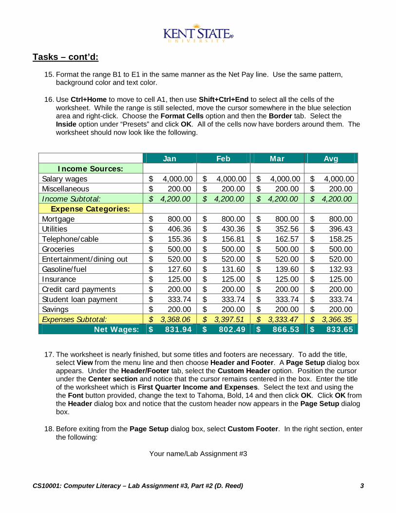
worksheet. While the range is still selected, move the cursor somewhere in the blue selection area and right-click. Choose the Format Cells option and then the Border tab. Select the Inside option under “Presets” and click OK. All of the cells now have borders around them. The worksheet should now look like the following.

Jan Feb Mar Avg Income Sources:

Salary wages $ 4,000.00 $ 4,000.00 $ 4,000.00 $ 4,000.00 Miscellaneous $ 200.00 $ 200.00 $ 200.00 $ 200.00 Income Subtotal: $ 4,200.00 $ 4,200.00 $ 4,200.00 $ 4,200.00

Expense Categories: Mortgage $ 800.00 $ 800.00 $ 800.00 $ 800.00 Utilities $ 406.36 $ 430.36 $ 352.56 $ 396.43 Telephone/cable $ 155.36 $ 156.81 $ 162.57 $ 158.25 Groceries $ 500.00 $ 500.00 $ 500.00 $ 500.00 Entertainment/dining out $ 520.00 $ 520.00 $ 520.00 $ 520.00 Gasoline/fuel $ 127.60 $ 131.60 $ 139.60 $ 132.93 Insurance $ 125.00 $ 125.00 $ 125.00 $ 125.00 Credit card payments $ 200.00 $ 200.00 $ 200.00 $ 200.00 Student loan payment $ 333.74 $ 333.74 $ 333.74 $ 333.74 Savings $ 200.00 $ 200.00 $ 200.00 $ 200.00 Expenses Subtotal: $ 3,368.06 $ 3,397.51 $ 3,333.47 $ 3,366.35

Net Wages: $ 831.94 $ 802.49 $ 866.53 $ 833.65

17. The worksheet is nearly finished, but some titles and footers are necessary. To add the title, select View from the menu line and then choose Header and Footer. A Page Setup dialog box appears. Under the Header/Footer tab, select the Custom Header option. Position the cursor under the Center section and notice that the cursor remains centered in the box. Enter the title of the worksheet which is First Quarter Income and Expenses. Select the text and using the the Font button provided, change the text to Tahoma, Bold, 14 and then click OK. Click OK from the Header dialog box and notice that the custom header now appears in the Page Setup dialog box.

18. Before exiting from the Page Setup dialog box, select Custom Footer. In the right section, enter

the following:

Your name/Lab Assignment #3

CS10001: Computer Literacy – Lab Assignment #3, Part #2 (D. Reed) 4

Tasks – cont’d: Use the default font and justification provided. Click OK when finished and then OK again to exit the Page Setup dialog box. The title and footer just created will not be visible from the worksheet, but if you select File Print Preview you will see them both. Select Close to return to the worksheet. 19. At the bottom of the worksheet is a tab with a label of Sheet 1. Position the cursor over the text

and right-click. Choose the option to Rename, name the worksheet First Quarter 2009, and enter. The cursor automatically moves inside the worksheet. Save the worksheet using Ctrl+S.

Steps – Chart:

1. Next is to create a chart showing only the monthly expenses. Select the range A1 through D16. While the range is selected, click on the Chart Wizard icon located on the Standard toolbar. A Chart Wizard dialog box appears with step 1 of 4. Use the chart type and chart subtype provided (Column and Clustered Column) by selecting Next.

2. The wizard’s step 2 of 4 uses a default data range with a Series in of “Columns”. Change the

Series in from “Columns” to “Rows”. The new chart arrangement is displayed; select Next to continue.

3. The wizard’s step 3 of 4 provides a place to insert a chart title. Use First Quarter Expenses for

the title and select Next to continue. At the wizard’s fourth step, select Finish. 4. The chart is positioned over the worksheet information and is selected as the active object (notice

the squares along the chart’s perimeter). To move the chart, position the cursor inside the white area of the chart and drag it to a new location while holding down the left mouse key. Position the chart at line 22 and center it underneath the worksheet information.

5. The chart contains all the information from the budget worksheet, but only the expenses are

required for the final chart. Some categories will need to be deleted. The first three bars on the chart represent the income values and income subtotal. To delete these, position the cursor over the first bar in January and left-click. A blue square appears at the center of the bar to show that the bar is selected; hit the Delete key. Delete the next two bars on the graph by repeating the steps above.

6. The chart now displays all of the monthly expenses, but the legend to the right of the chart must

be updated. Select the text “Income Sources:” inside the legend and delete the text. Select the “Expense Categories:” text inside the legend and delete it. The first expense (Mortgage) is now the first item in the chart’s legend. Save the chart and worksheet by using Ctrl+S.

7. A new print range will need to be set to include the chart along with the worksheet. At cell A1,

hold down the left mouse key and drag to select the range of A1 through E37. Select File Print Area Set Print Area and notice that the worksheet and the chart are included in the selection. Save the worksheet by using Ctrl+S. Select File Print Preview to view the final worksheet and chart. Select Close to return to the worksheet and chart.

CS10001: Computer Literacy – Lab Assignment #3, Part #2 (D. Reed) 5

Steps – Chart (cont’d):

8. Close the Excel application and upload this file to your account on the research.kent.edu server. Place it in your CS10001 folder (inside the public_html folder). You will be prompted to overwrite or replace the current server file, so select OK.

9. Set the correct file permissions for the file. Failure to do this step may result in your files being

inaccessible via a web browser. Check for a successful upload by opening a browser and using the following URL (replace the userid with your FlashLine userid).

Example: http://www.personal.kent.edu/~userid/CS10001/budget.xls

10. The due date for this part of the lab is Tuesday, March 10, 2009 by 5:00 p.m.