Embed Size (px)
Citation preview
CS 775: Advanced Computer Graphics
Lecture 12: Fluid SimulationGrid Fluids
CS 775: Lecture 12 Parag Chaudhuri, 2015
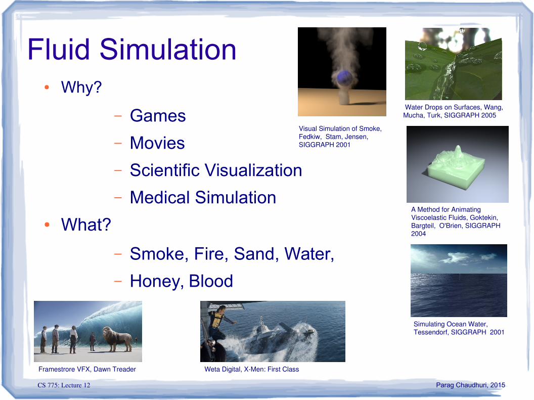
Fluid Simulation● Why?
– Games
– Movies
– Scientific Visualization
– Medical Simulation● What?
– Smoke, Fire, Sand, Water,
– Honey, Blood
Water Drops on Surfaces, Wang, Mucha, Turk, SIGGRAPH 2005
A Method for Animating Viscoelastic Fluids, Goktekin, Bargteil, O'Brien, SIGGRAPH 2004
Simulating Ocean Water, Tessendorf, SIGGRAPH 2001
Visual Simulation of Smoke, Fedkiw, Stam, Jensen, SIGGRAPH 2001
Framestrore VFX, Dawn Treader Weta Digital, XMen: First Class
CS 775: Lecture 12 Parag Chaudhuri, 2015
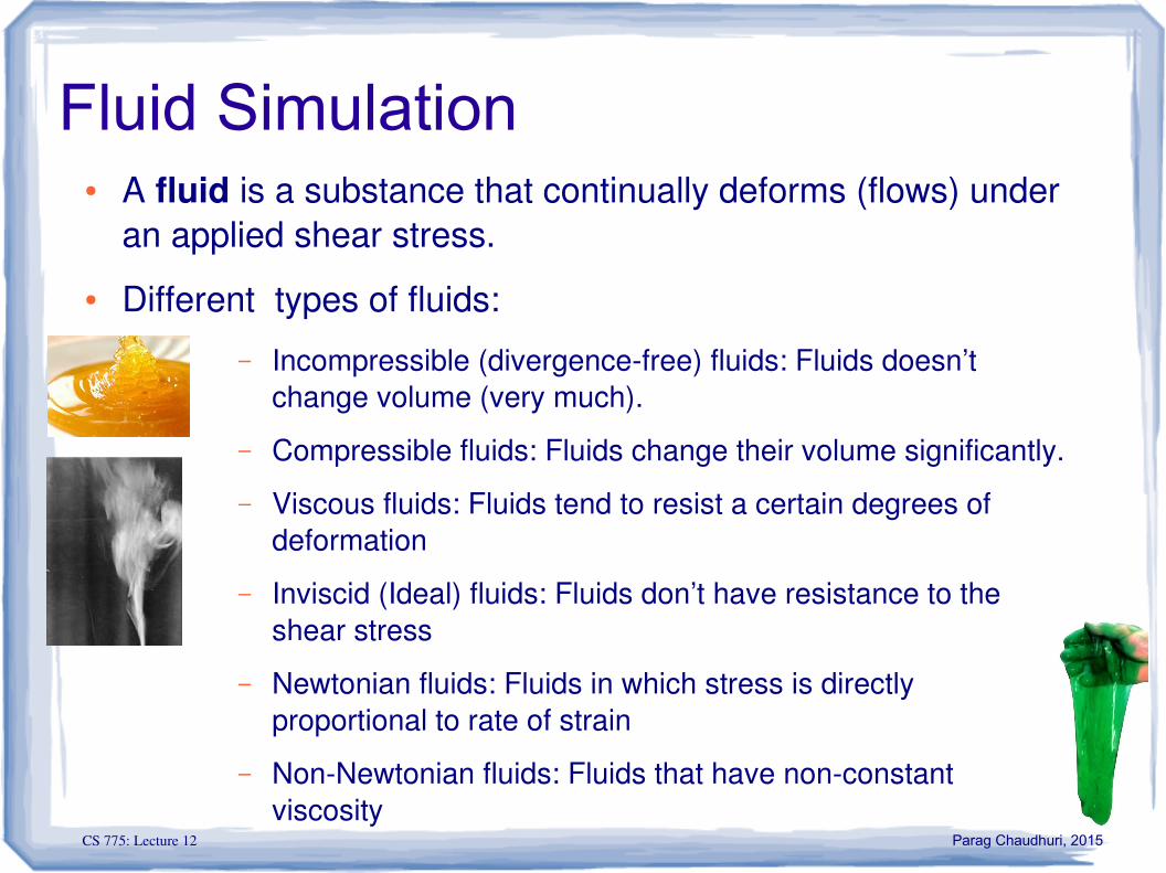
Fluid Simulation● A fluid is a substance that continually deforms (flows) under
an applied shear stress.
● Different types of fluids:
– Incompressible (divergencefree) fluids: Fluids doesn’t change volume (very much).
– Compressible fluids: Fluids change their volume significantly.
– Viscous fluids: Fluids tend to resist a certain degrees of deformation
– Inviscid (Ideal) fluids: Fluids don’t have resistance to the shear stress
– Newtonian fluids: Fluids in which stress is directly proportional to rate of strain
– NonNewtonian fluids: Fluids that have nonconstant viscosity
CS 775: Lecture 12 Parag Chaudhuri, 2015
Fluid Simulation
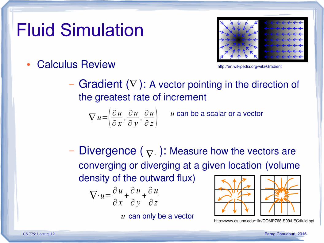
● Calculus Review
– Gradient ( ): A vector pointing in the direction of the greatest rate of increment
– Divergence ( ): Measure how the vectors are converging or diverging at a given location (volume density of the outward flux)
∇
can be a scalar or a vectoru∇ u=( ∂u∂ x,∂u∂ y,∂u∂ z )
http://en.wikipedia.org/wiki/Gradient
∇⋅
http://www.cs.unc.edu/~lin/COMP768S09/LEC/fluid.ppt
∇⋅u=∂ u∂ x
+∂ u∂ y
+∂ u∂ z
can only be a vectoru
CS 775: Lecture 12 Parag Chaudhuri, 2015
Fluid Simulation
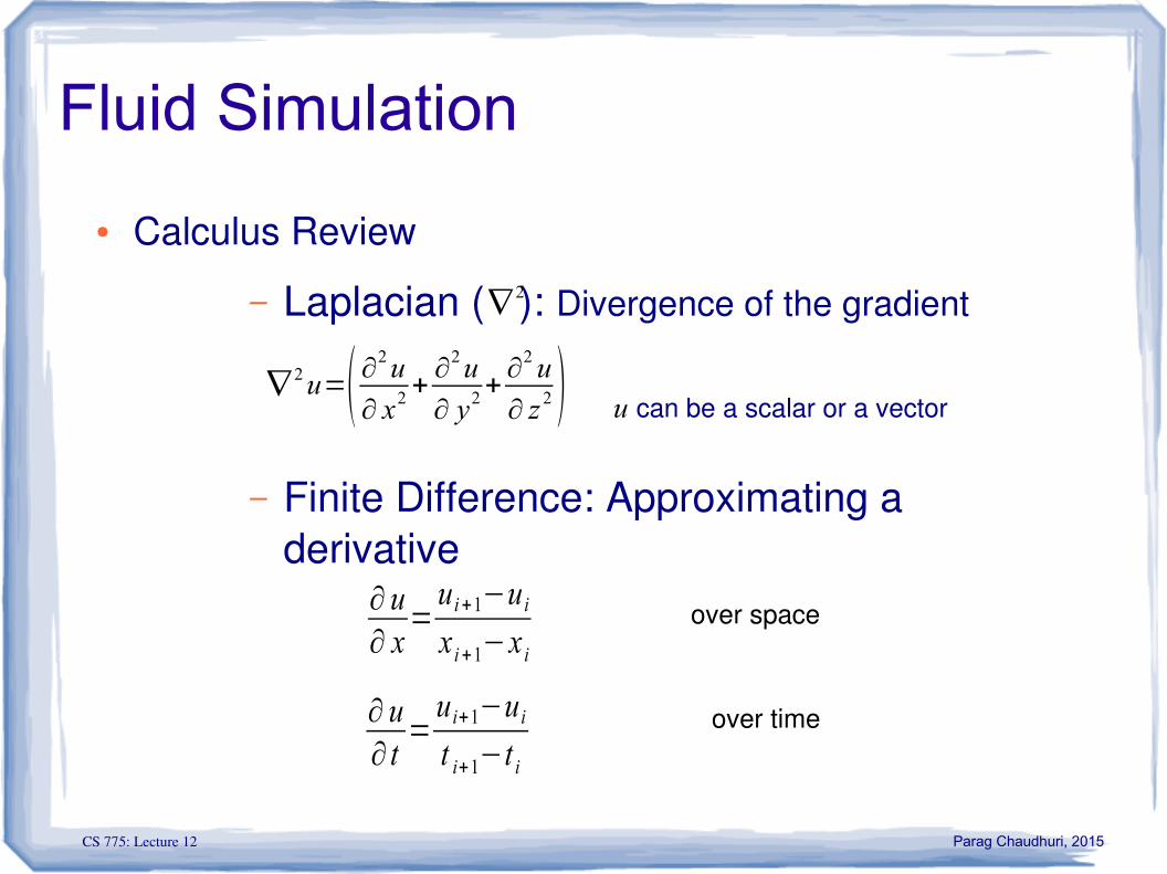
● Calculus Review
– Laplacian ( ): Divergence of the gradient
– Finite Difference: Approximating a derivative
∇2
can be a scalar or a vectoru∇ 2u=( ∂
2u
∂ x2 +∂
2u
∂ y2 +∂
2u
∂ z 2 )
∂ u∂ x
=ui+1−u ix i+1−x i
∂ u∂ t
=u i+1−u it i+1−t i
over space
over time
CS 775: Lecture 12 Parag Chaudhuri, 2015
Fluid Simulation
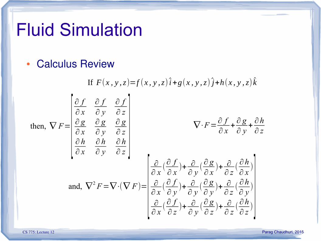
● Calculus Review
then, ∇ F=[∂ f∂ x
∂ f∂ y
∂ f∂ z
∂ g∂ x
∂ g∂ y
∂ g∂ z
∂ h∂ x
∂ h∂ y
∂ h∂ z
] ∇⋅F=∂ f∂ x
+∂ g∂ y
+∂h∂ z
If F (x , y , z)=f (x , y , z) i+g(x , y , z) j+h(x , y , z) k
and, ∇2F=∇⋅(∇ F )=[∂∂ x
(∂ f∂ x
)+ ∂∂ y
(∂ g∂ x
)+ ∂∂ z
(∂h∂ x
)
∂∂ x
(∂ f∂ y
)+ ∂∂ y
(∂ g∂ y
)+ ∂∂ z
(∂h∂ y
)
∂∂ x
(∂ f∂ z
)+ ∂∂ y
(∂ g∂ z
)+ ∂∂ z
(∂h∂ z
)]
CS 775: Lecture 12 Parag Chaudhuri, 2015
Fluid Simulation
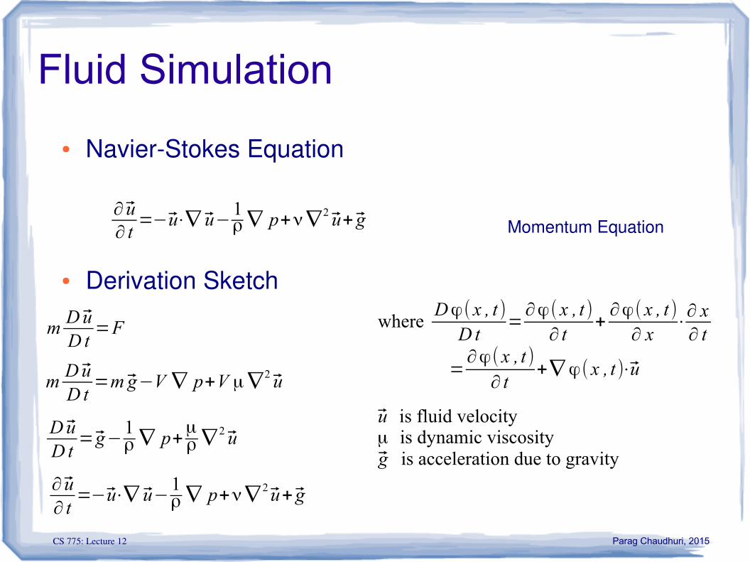
● NavierStokes Equation
● Derivation Sketch
∂ u∂ t
=−u⋅∇ u−1ρ ∇ p+ν∇
2 u+ g Momentum Equation
mD uD t
=F where Dϕ( x , t )Dt
=∂ϕ( x , t )
∂ t+
∂ϕ( x , t )∂ x
⋅∂ x∂ t
=∂ϕ( x , t )
∂ t+∇ ϕ( x , t )⋅u
mD uD t
=m g−V ∇ p+V μ ∇2 u
D uD t
= g−1ρ ∇ p+
μρ ∇
2 u
∂ u∂ t
=−u⋅∇ u−1ρ ∇ p+ν∇
2 u+ g
u is fluid velocityμ is dynamic viscosityg is acceleration due to gravity
CS 775: Lecture 12 Parag Chaudhuri, 2015
Fluid Simulation
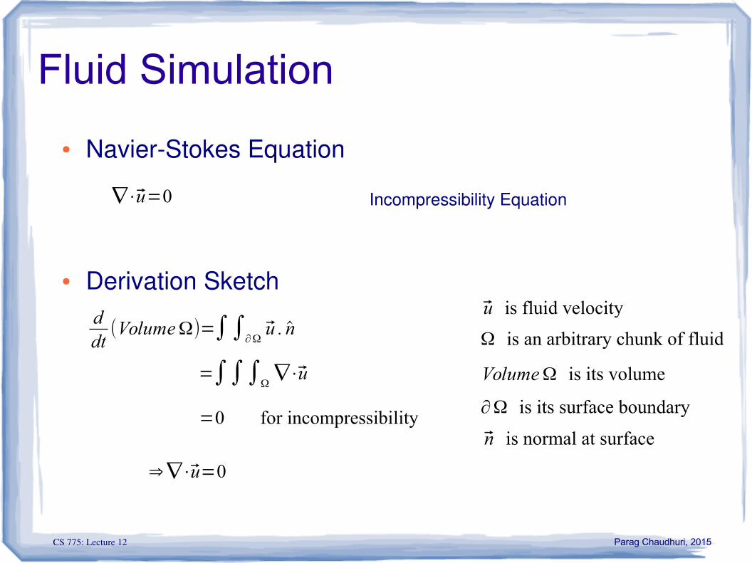
● NavierStokes Equation
● Derivation Sketch
∇⋅u=0 Incompressibility Equation
u is fluid velocity
Ω is an arbitrary chunk of fluid
n is normal at surface
ddt
(VolumeΩ)=∫∫∂Ωu . n
=∫∫∫Ω∇⋅u
=0 for incompressibility
⇒∇⋅u=0
VolumeΩ is its volume
∂Ω is its surface boundary
CS 775: Lecture 12 Parag Chaudhuri, 2015
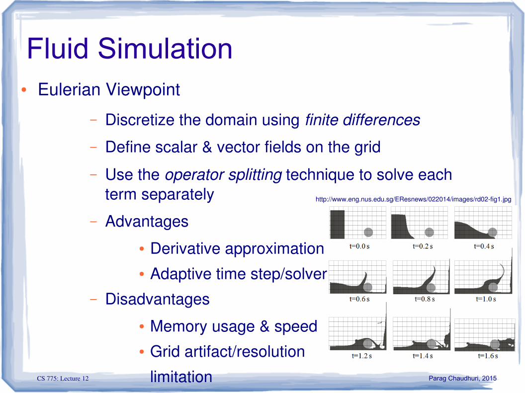
Fluid Simulation● Eulerian Viewpoint
– Discretize the domain using finite differences
– Define scalar & vector fields on the grid
– Use the operator splitting technique to solve each term separately
– Advantages● Derivative approximation● Adaptive time step/solver
– Disadvantages● Memory usage & speed● Grid artifact/resolution
limitation
http://www.eng.nus.edu.sg/EResnews/022014/images/rd02fig1.jpg
CS 775: Lecture 12 Parag Chaudhuri, 2015
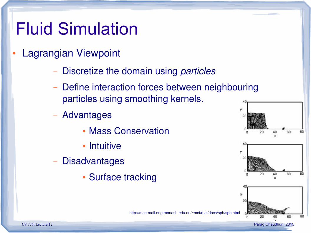
Fluid Simulation● Lagrangian Viewpoint
– Discretize the domain using particles
– Define interaction forces between neighbouring particles using smoothing kernels.
– Advantages● Mass Conservation● Intuitive
– Disadvantages● Surface tracking
http://mecmail.eng.monash.edu.au/~mct/mct/docs/sph/sph.html
CS 775: Lecture 12 Parag Chaudhuri, 2015
Fluid Simulation
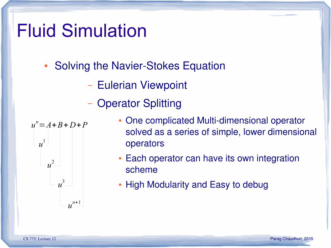
● Solving the NavierStokes Equation
– Eulerian Viewpoint
– Operator Splitting● One complicated Multidimensional operator
solved as a series of simple, lower dimensional operators
● Each operator can have its own integration scheme
● High Modularity and Easy to debug
un=A+B+D+P
u2
u1
u3
un+1
CS 775: Lecture 12 Parag Chaudhuri, 2015
Fluid Simulation
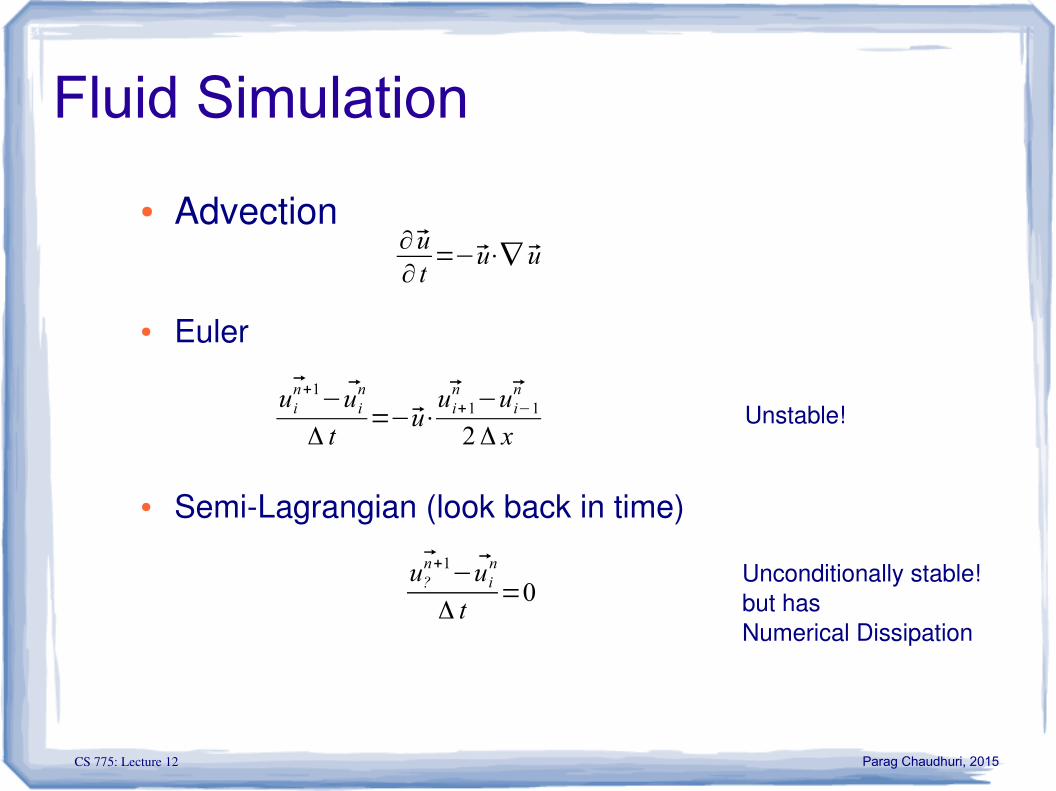
● Advection
● Euler
● SemiLagrangian (look back in time)
∂ u∂ t
=−u⋅∇ u
uin+1−ui
n
Δ t=−u⋅
ui+1n − ui−1
n
2 Δ xUnstable!
u?n+1−ui
n
Δ t=0
Unconditionally stable!but hasNumerical Dissipation
CS 775: Lecture 12 Parag Chaudhuri, 2015
Fluid Simulation
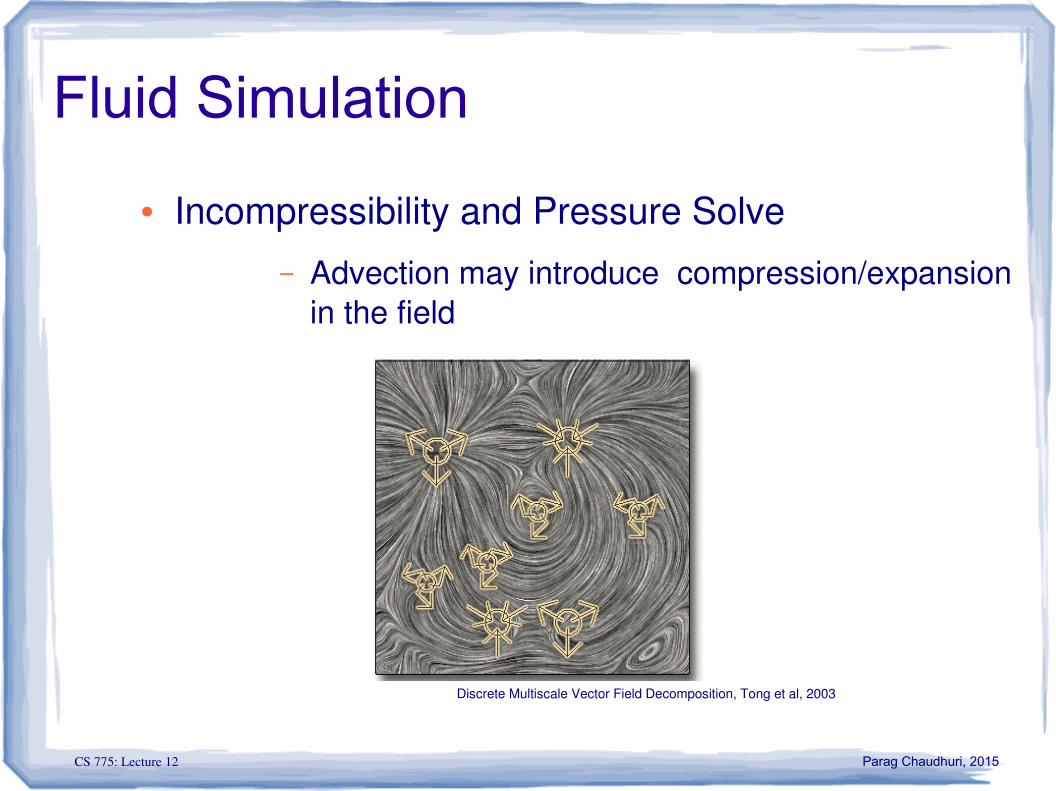
● Incompressibility and Pressure Solve– Advection may introduce compression/expansion
in the field
Discrete Multiscale Vector Field Decomposition, Tong et al, 2003
CS 775: Lecture 12 Parag Chaudhuri, 2015
Fluid Simulation
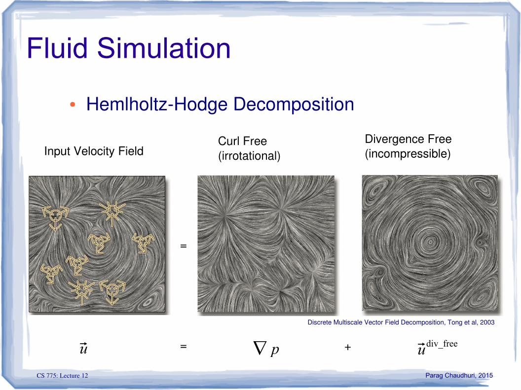
● HemlholtzHodge Decomposition
Discrete Multiscale Vector Field Decomposition, Tong et al, 2003
=
+u ∇ p udiv_free
Input Velocity FieldCurl Free (irrotational)
Divergence Free (incompressible)
=
CS 775: Lecture 12 Parag Chaudhuri, 2015
Fluid Simulation
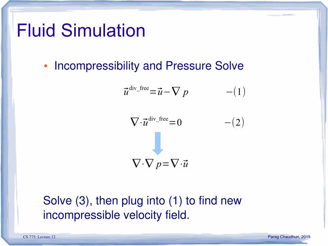
● Incompressibility and Pressure Solve
udiv_free=u−∇ p −(1)
∇⋅udiv_free=0 −(2)
∇⋅∇ p=∇⋅u
Solve (3), then plug into (1) to find new incompressible velocity field.
CS 775: Lecture 12 Parag Chaudhuri, 2015
Fluid Simulation
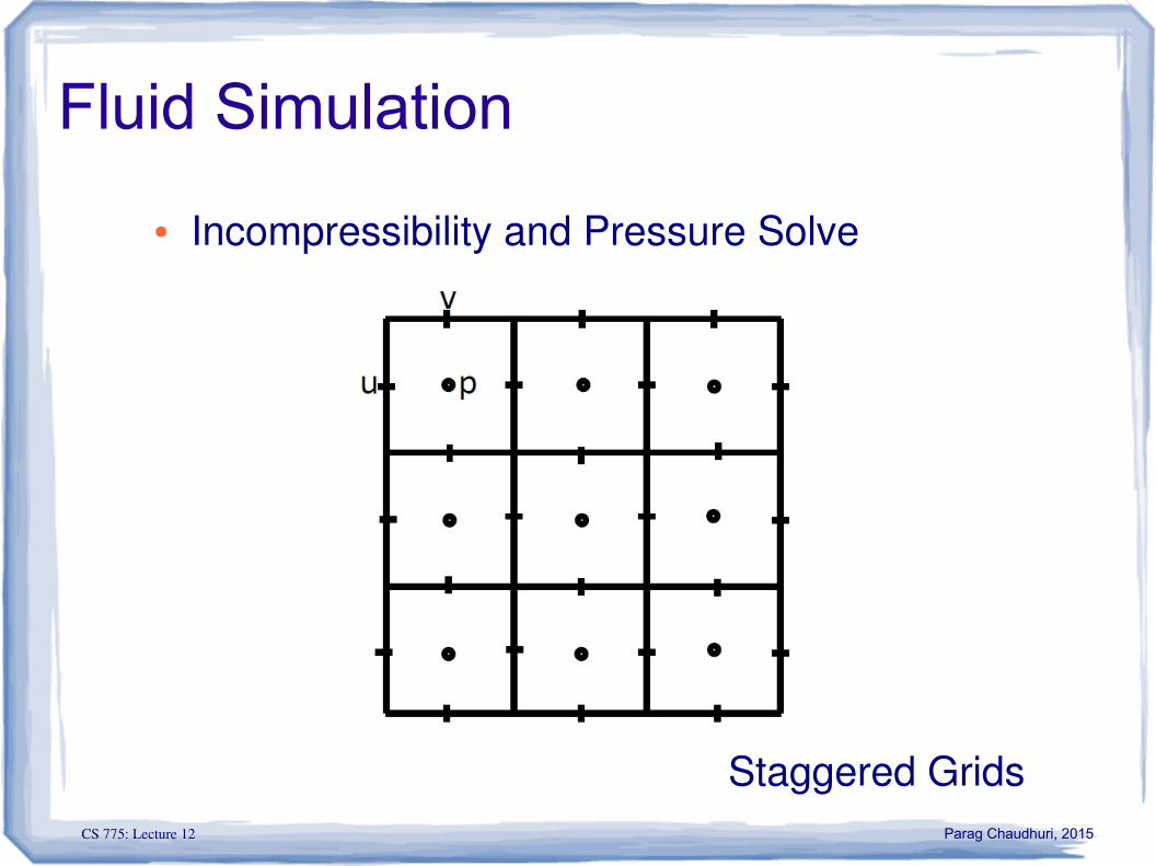
● Incompressibility and Pressure Solve
Staggered Grids
CS 775: Lecture 12 Parag Chaudhuri, 2015
Fluid Simulation
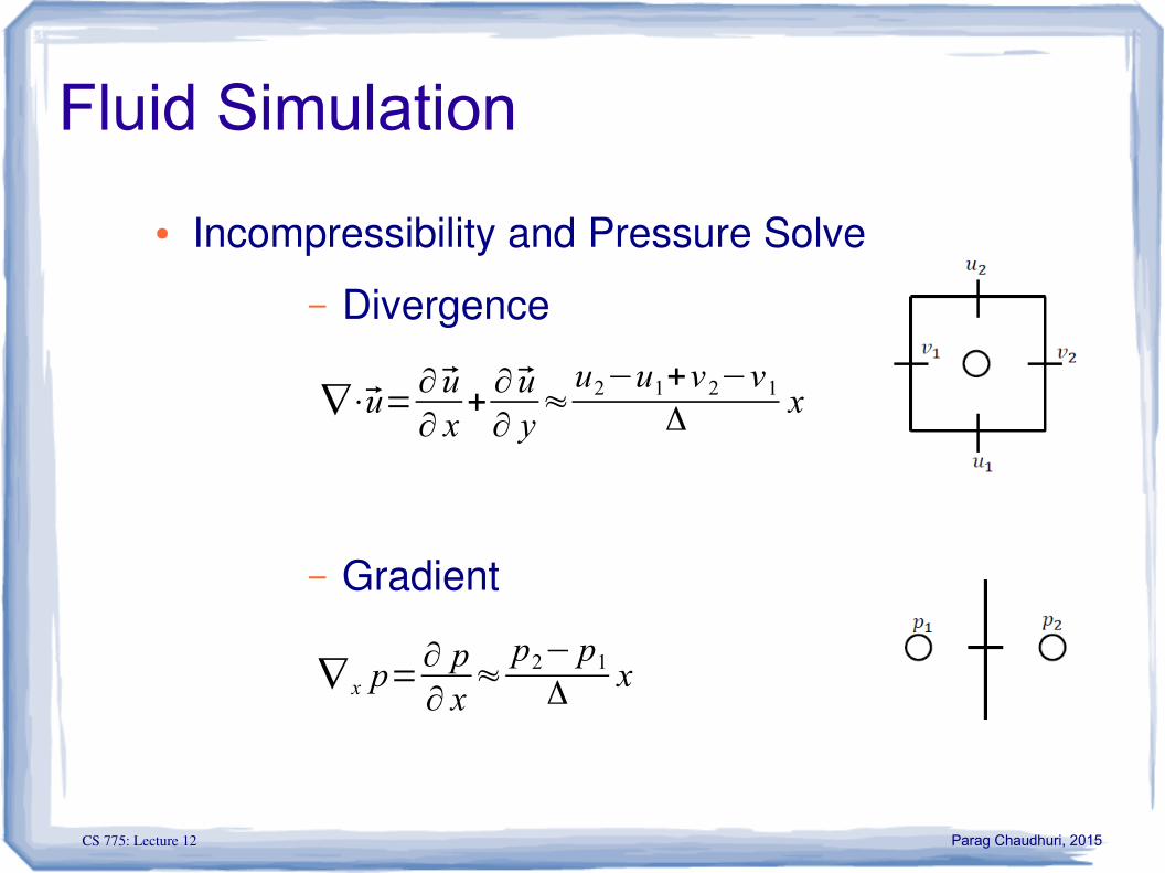
● Incompressibility and Pressure Solve
– Divergence
– Gradient
∇⋅u=∂ u∂ x
+∂ u∂ y
≈u2−u1+v2−v1
Δx
∇ x p=∂ p∂ x
≈p2− p1
Δx
CS 775: Lecture 12 Parag Chaudhuri, 2015
Fluid Simulation
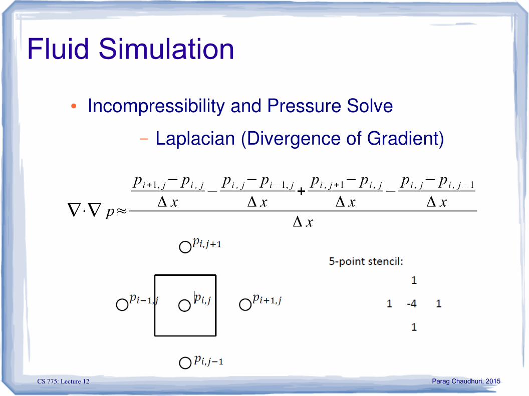
● Incompressibility and Pressure Solve
– Laplacian (Divergence of Gradient)
∇⋅∇ p≈
pi+1, j− pi , jΔ x
−pi , j− pi−1, j
Δ x+pi , j+1− p i , j
Δ x−pi , j− pi , j−1
Δ xΔ x
CS 775: Lecture 12 Parag Chaudhuri, 2015
Fluid Simulation
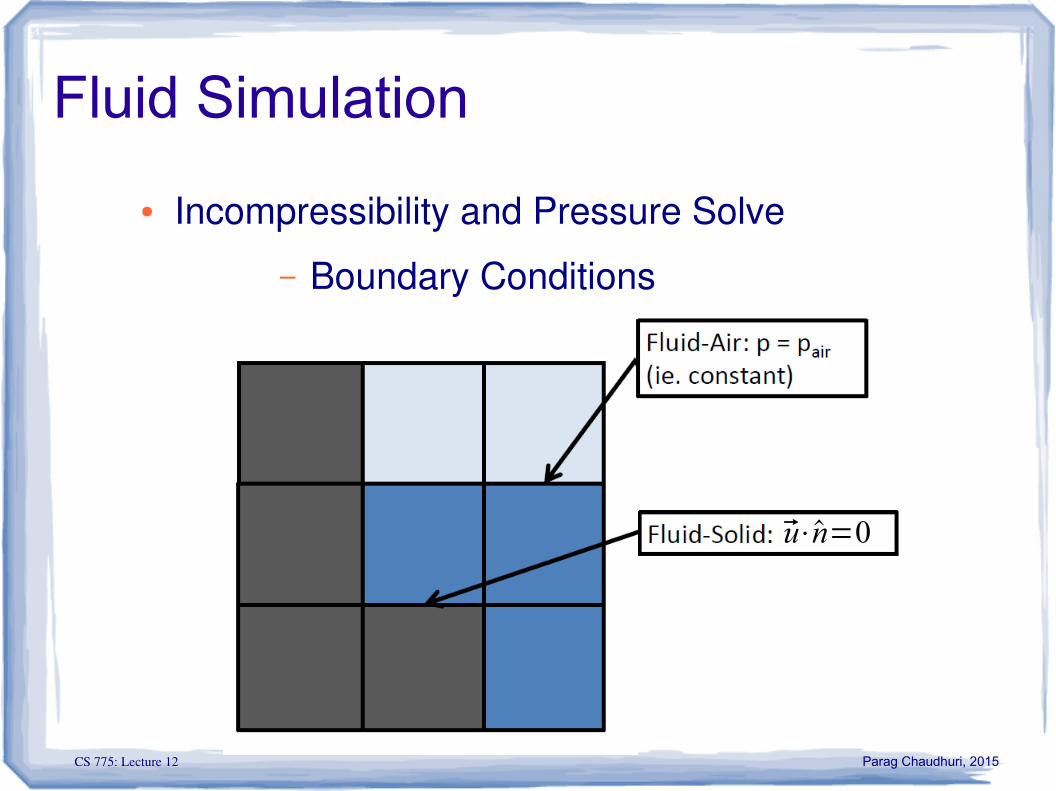
● Incompressibility and Pressure Solve
– Boundary Conditions
u⋅n=0
CS 775: Lecture 12 Parag Chaudhuri, 2015
Fluid Simulation
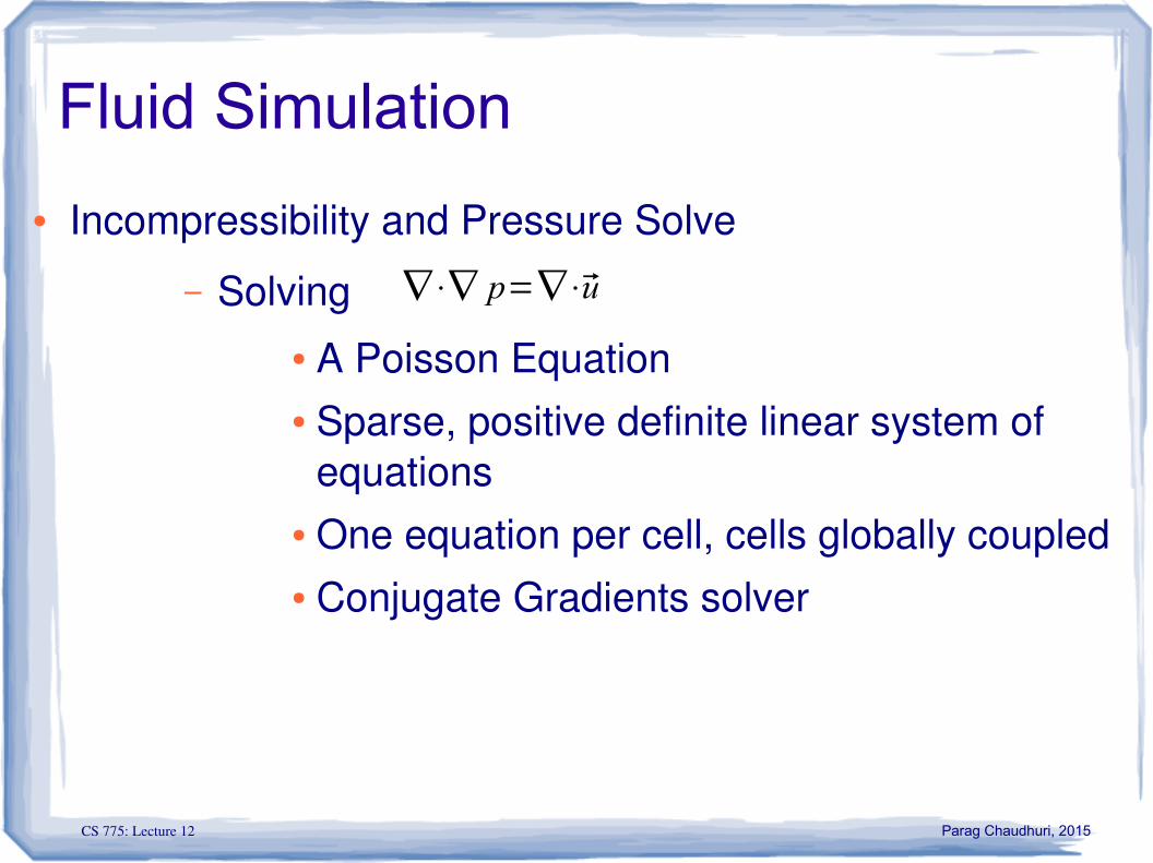
● Incompressibility and Pressure Solve
– Solving● A Poisson Equation● Sparse, positive definite linear system of
equations● One equation per cell, cells globally coupled● Conjugate Gradients solver
∇⋅∇ p=∇⋅u
CS 775: Lecture 12 Parag Chaudhuri, 2015
Fluid Simulation
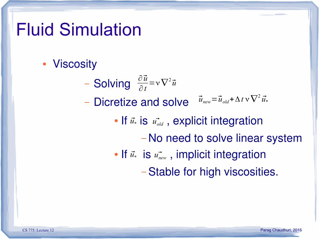
● Viscosity
– Solving– Dicretize and solve
● If is , explicit integration– No need to solve linear system
● If is , implicit integration– Stable for high viscosities.
∂ u∂ t
=ν∇2 u
unew= uold+Δ t ν∇2 u*
u*
u* unew
uold
CS 775: Lecture 12 Parag Chaudhuri, 2015
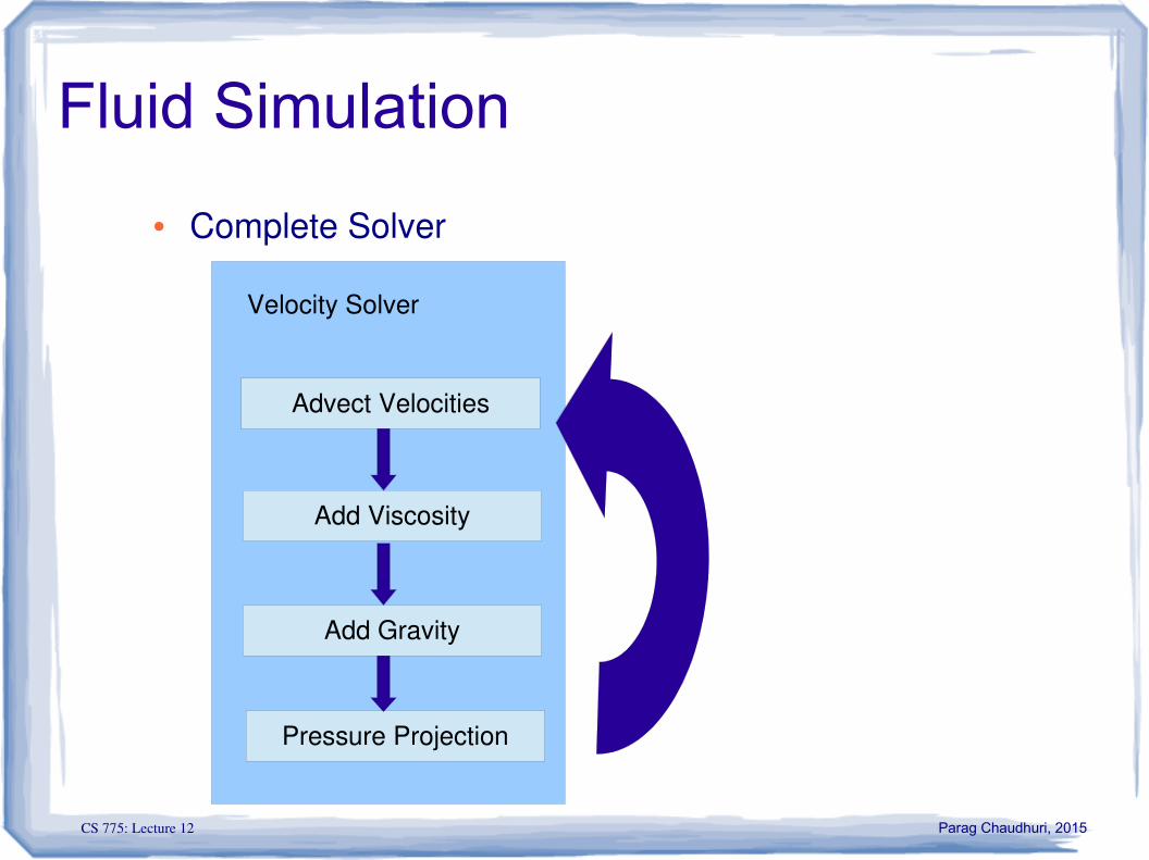
Fluid Simulation
● Complete Solver
Velocity Solver
Advect Velocities
Add Viscosity
Add Gravity
Pressure Projection
CS 775: Lecture 12 Parag Chaudhuri, 2015
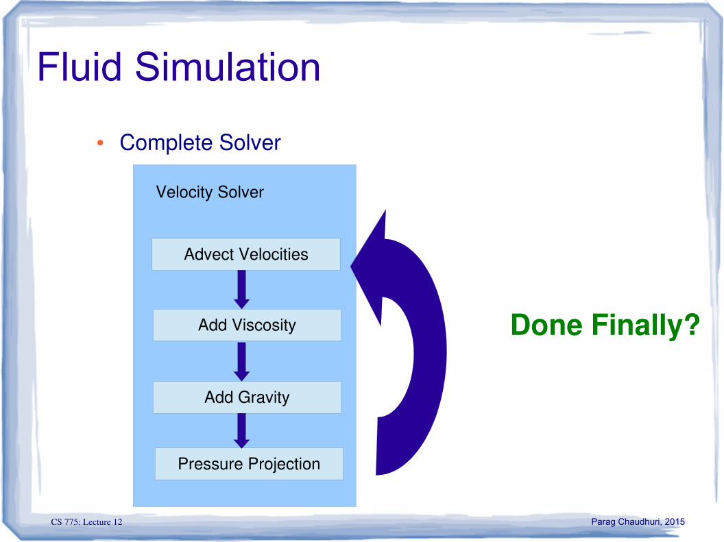
Fluid Simulation
● Complete Solver
Velocity Solver
Advect Velocities
Add Viscosity
Add Gravity
Pressure Projection
Done Finally?
CS 775: Lecture 12 Parag Chaudhuri, 2015
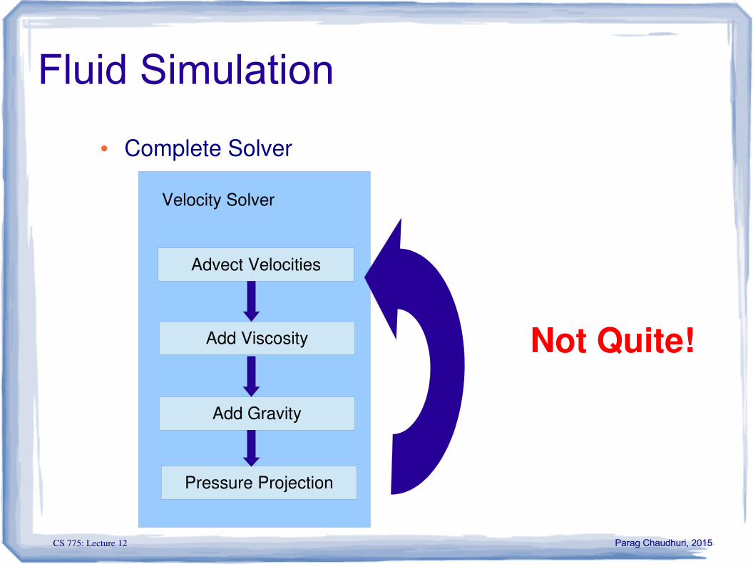
Fluid Simulation
● Complete Solver
Velocity Solver
Advect Velocities
Add Viscosity
Add Gravity
Pressure Projection
Not Quite!
CS 775: Lecture 12 Parag Chaudhuri, 2015
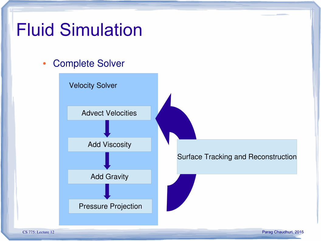
Fluid Simulation
● Complete Solver
Velocity Solver
Advect Velocities
Add Viscosity
Add Gravity
Pressure Projection
Surface Tracking and Reconstruction