Embed Size (px)
Citation preview
CS 598: Spectral Graph
Theory. Lecture 1
The Laplacian
Alexandra Kolla

Administrativia
� Email, office, office hours, course
website, scribe notes, homeworks,
projects, prerequisites.
� Course goals.
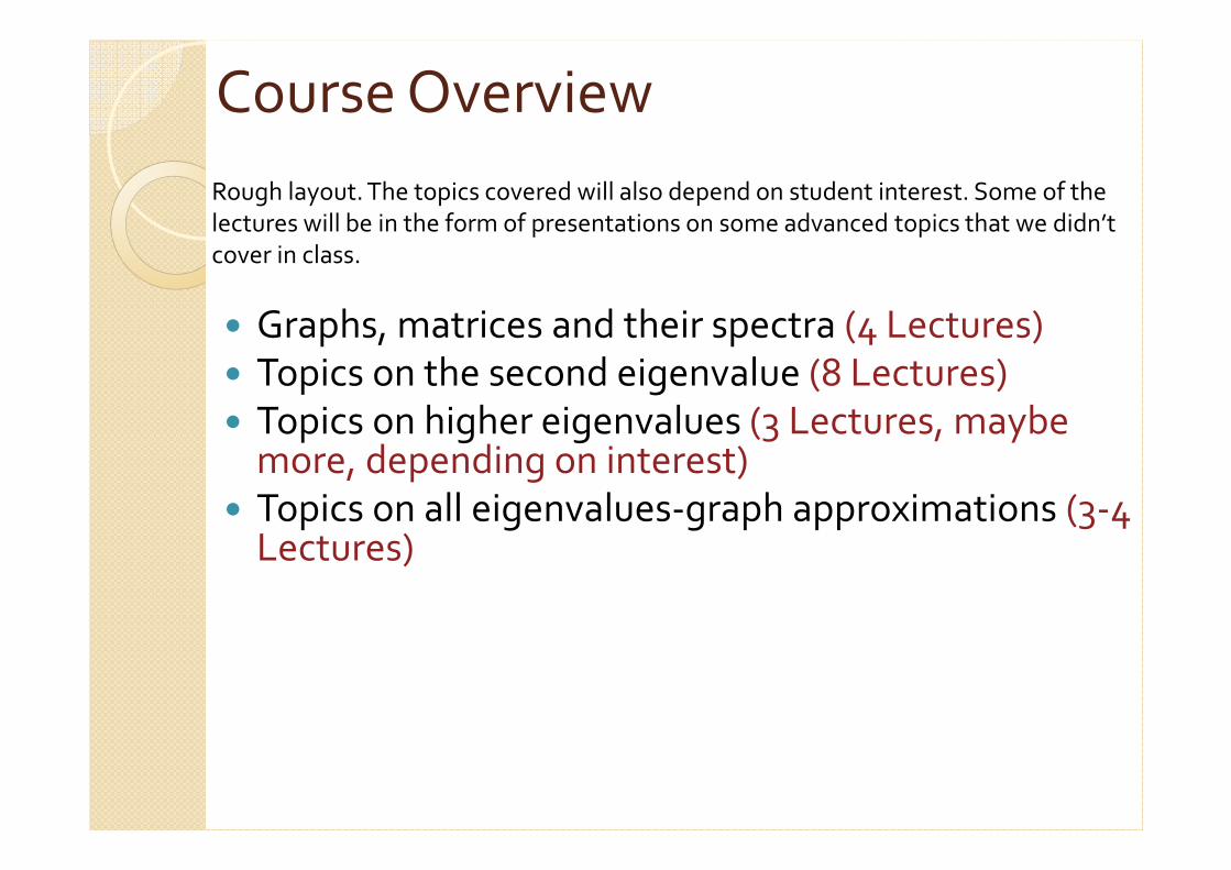
Course Overview
� Graphs, matrices and their spectra (4 Lectures)� Topics on the second eigenvalue (8 Lectures)� Topics on higher eigenvalues (3 Lectures, maybe
more, depending on interest)� Topics on all eigenvalues-graph approximations (3-4
Lectures)
Rough layout. The topics covered will also depend on student interest. Some of the
lectures will be in the form of presentations on some advanced topics that we didn’t
cover in class.
Graphs, Matrices and their Spectra
� Adjacency matrix, diffusion operator, Laplacian.
� Eigenvalues and eigenvectors of graphs, examples.
� Properties of the Laplacian, properties of adjacency matrix and their relations.
� Courant-Fischer, Perron-Frobenius, nodal domains.
� Eigenvalue bounding techniques, examples.
Topics on the Second Eigenvalue
� Edge expansion, graph cutting, Cheeger’s inequality.
� Semidefinite programming, duality and connections with the second eigenvalue.
� Second eigenvalue for planar graphs.
� Expanders: existence, constructions and applications.
Topics on Higher Eigenvalues
� Approximation algorithm for MAXCUT using the last eigenvalue.
� Small set expansion and higher eigenvalues, Cheeger-like inequalities.
� The Unique Games Conjecture and approximation algorithms using higher eigenvalues.
� Semidefinite programming hierarchies and higher spectra (maybe).
Topics on All Eigenvalues-Graph
Approximations
� Various graph approximations,
sparsification and applications.
� Spectral sparsifiers with effective
resistances.
� Solving Laplacian systems of linear
equations with preconditioning,
ultrasparsifiers.
In the next few minutes:
Why spectral graph theory is both natural
and magical
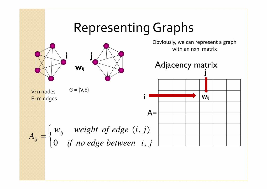
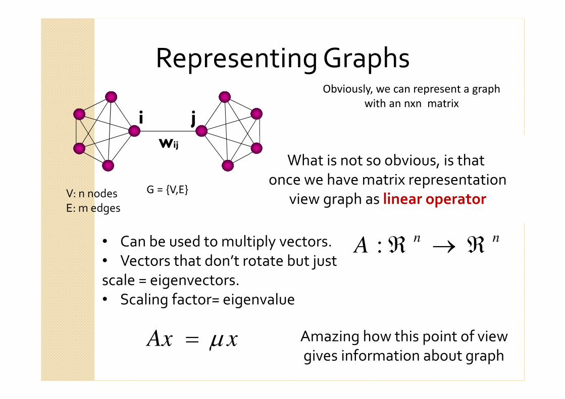
Representing Graphs
V: n nodes
E: m edges
G = {V,E}
Obviously, we can represent a graph
with an nxn matrix
wij
i j
wij
Adjacency matrixj
i
A=
=jibetweenedgenoif
jiedgeofweightwA
ij
ij,0
),(
Representing Graphs
V: n nodes
E: m edges
G = {V,E}
wij
i j
What is not so obvious, is that
once we have matrix representation
view graph as linear operator
xAx µ=
nnA ℜ→ℜ:• Can be used to multiply vectors.
• Vectors that don’t rotate but just
scale = eigenvectors.
• Scaling factor= eigenvalue
Amazing how this point of view
gives information about graph
Obviously, we can represent a graph
with an nxn matrix
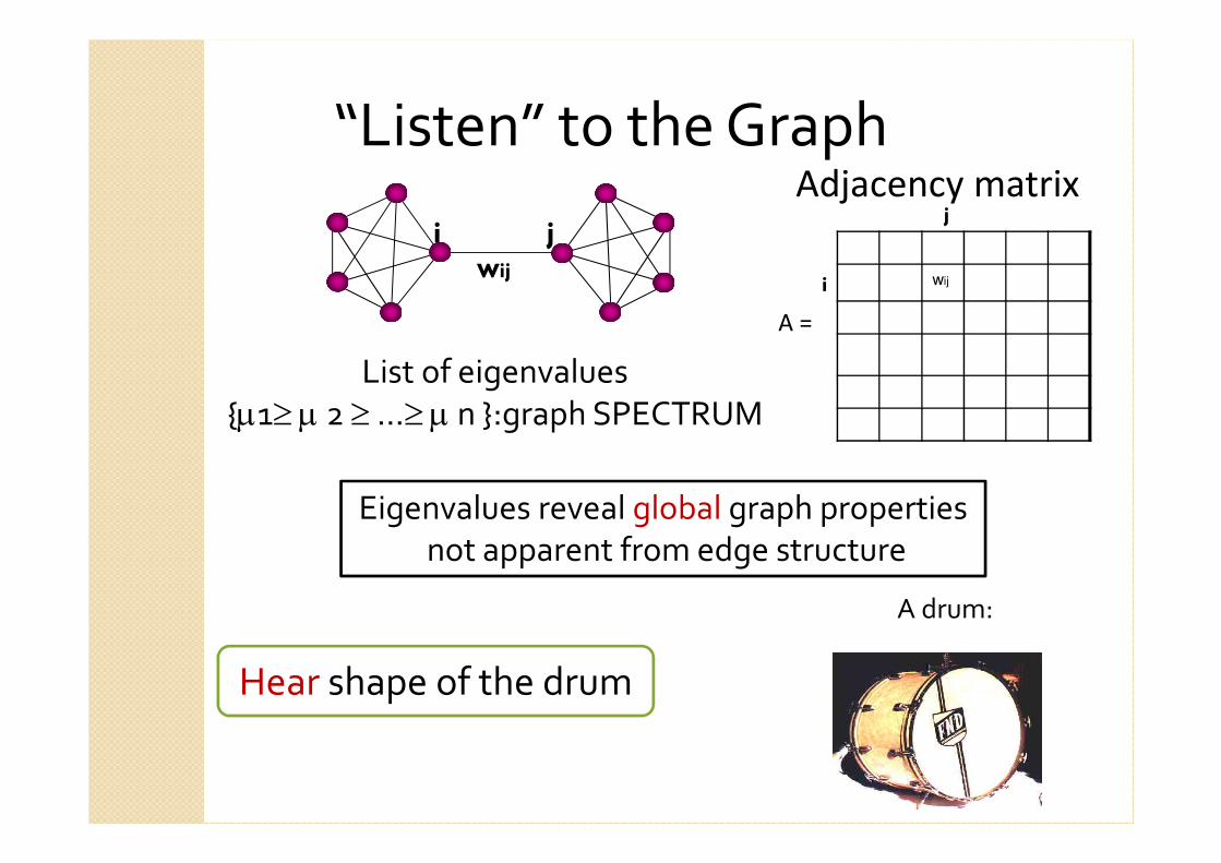
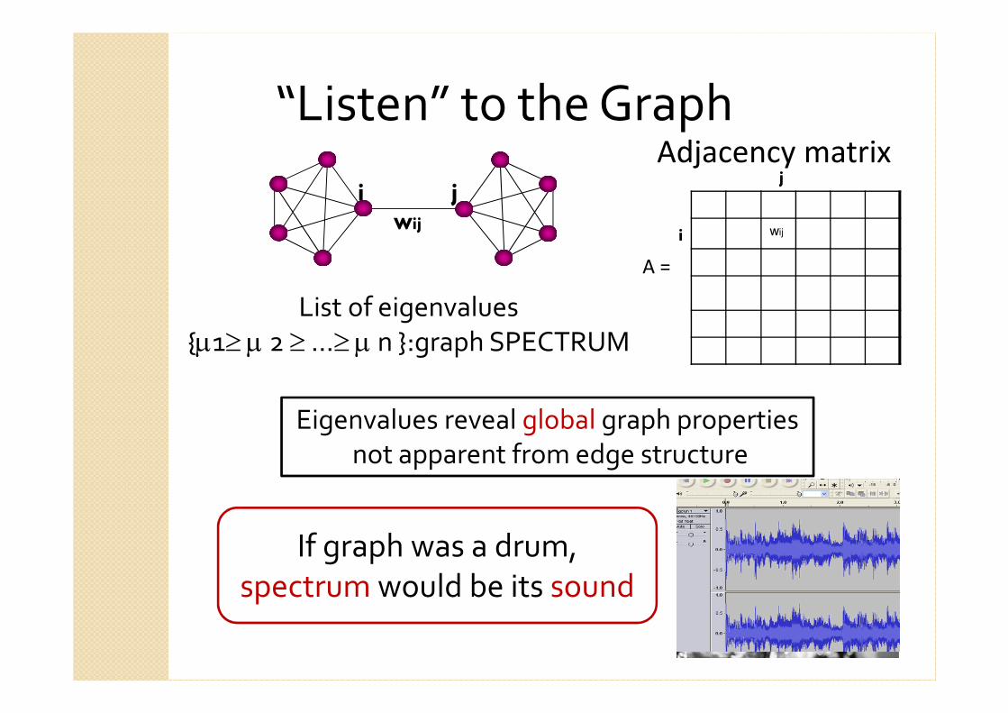
“Listen” to the Graph
List of eigenvalues
{µ1≥ µ 2 ≥…≥ µ n }:graph SPECTRUM
wiji j
Eigenvalues reveal global graph properties
not apparent from edge structure
Adjacency matrix
wij
j
i
A =
A drum:
Hear shape of the drum
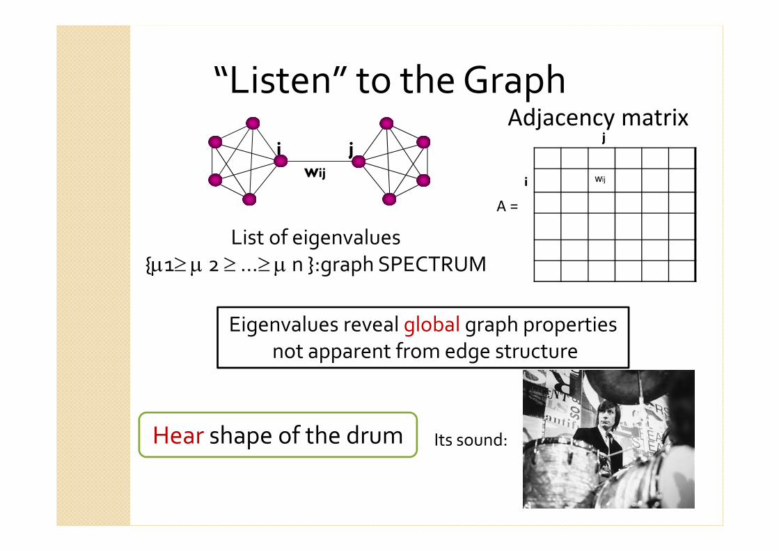
“Listen” to the Graph
List of eigenvalues
{µ1≥ µ 2 ≥…≥ µ n }:graph SPECTRUM
wiji j
Eigenvalues reveal global graph properties
not apparent from edge structure
Hear shape of the drum
Adjacency matrix
wij
j
i
A =
Its sound:
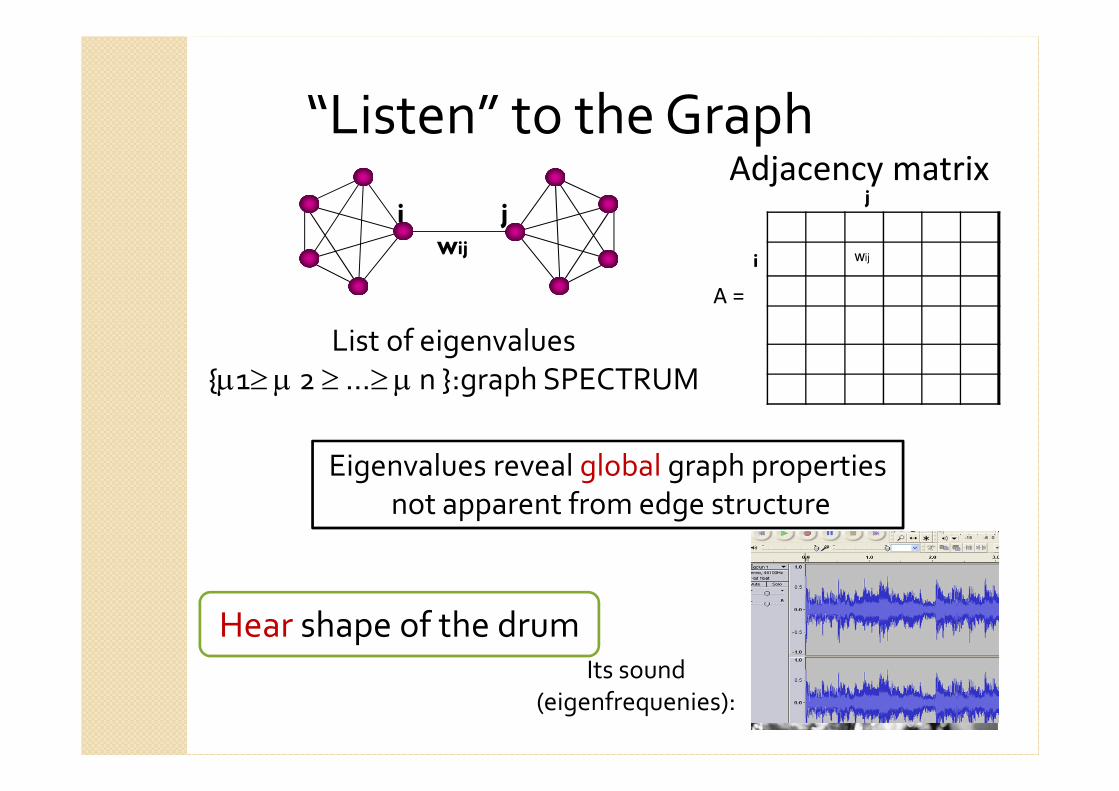
“Listen” to the Graph
List of eigenvalues
{µ1≥ µ 2 ≥…≥ µ n }:graph SPECTRUM
wiji j
Eigenvalues reveal global graph properties
not apparent from edge structure
Hear shape of the drum
Adjacency matrix
wij
j
i
A =
Its sound
(eigenfrequenies):
“Listen” to the Graph
List of eigenvalues
{µ1≥ µ 2 ≥…≥ µ n }:graph SPECTRUM
wiji j
Eigenvalues reveal global graph properties
not apparent from edge structure
Adjacency matrix
wij
j
i
A =
If graph was a drum,
spectrum would be its sound
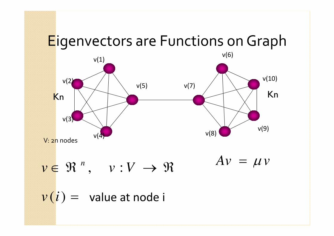
Eigenvectors are Functions on Graph
vAv µ=ℜ→ℜ∈ Vvvn
:,
=)(iv value at node i
v(2)
v(1)
v(3)
v(5)
v(4)V: 2n nodes
Kn Knv(7)
v(6)
v(8)
v(10)
v(9)
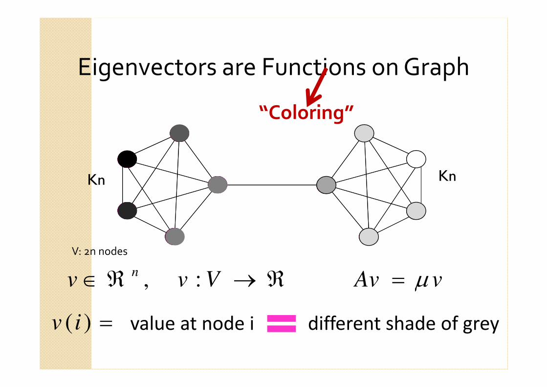
Eigenvectors are Functions on Graph
V: 2n nodes
Kn Kn
“Coloring”
vAv µ=ℜ→ℜ∈ Vvvn
:,
=)(iv value at node i different shade of grey
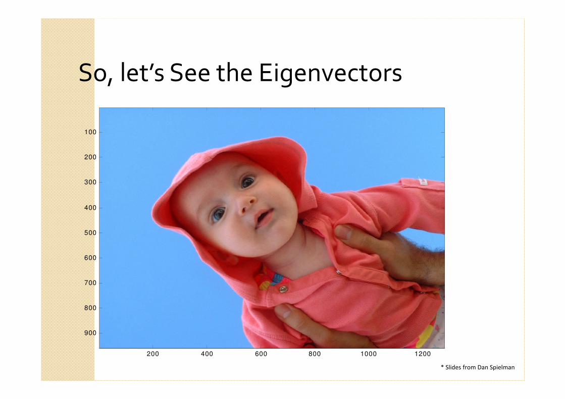
So, let’s See the Eigenvectors
200 400 600 800 1000 1200
100
200
300
400
500
600
700
800
900
* Slides from Dan Spielman
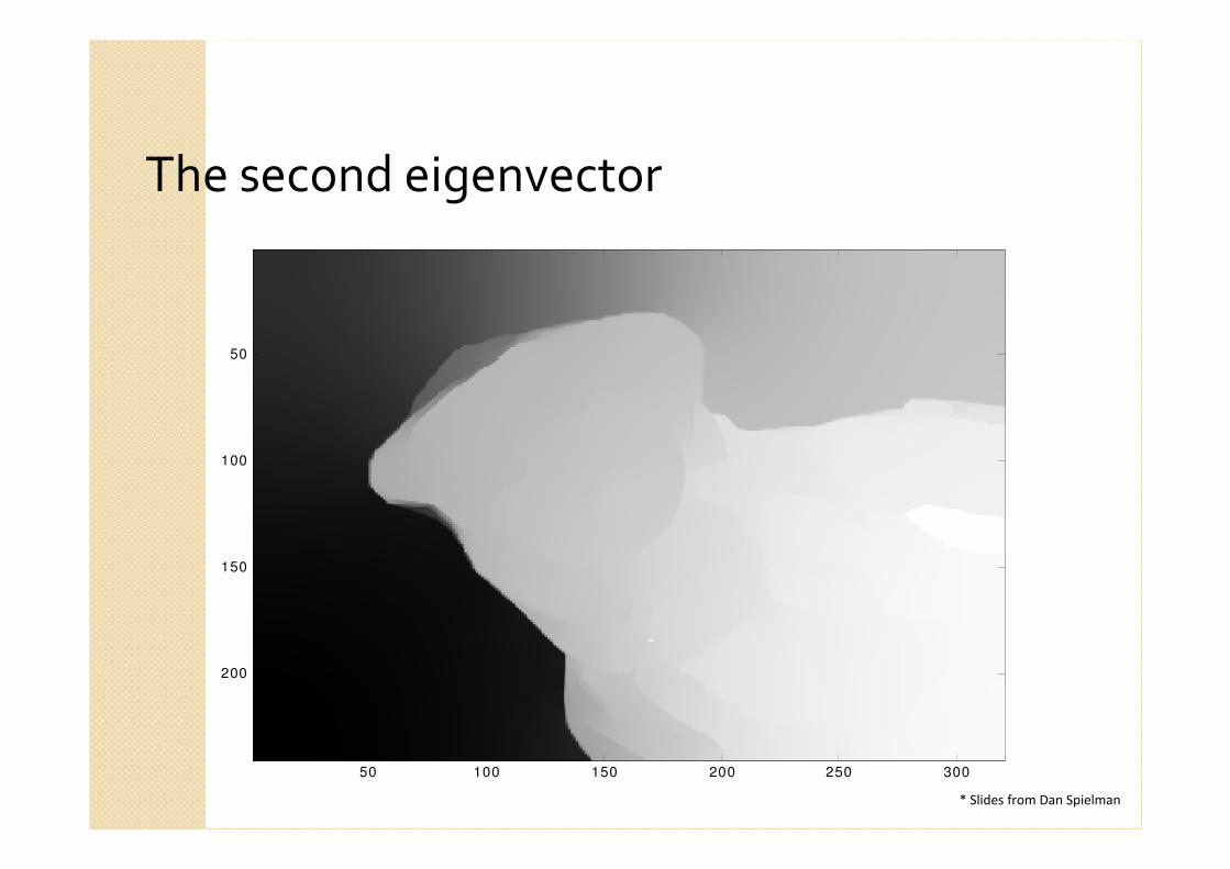
The second eigenvector
50 100 150 200 250 300
50
100
150
200
* Slides from Dan Spielman
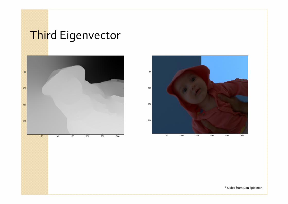
Third Eigenvector
50 100 150 200 250 300
50
100
150
200
50 100 150 200 250 300
50
100
150
200
* Slides from Dan Spielman
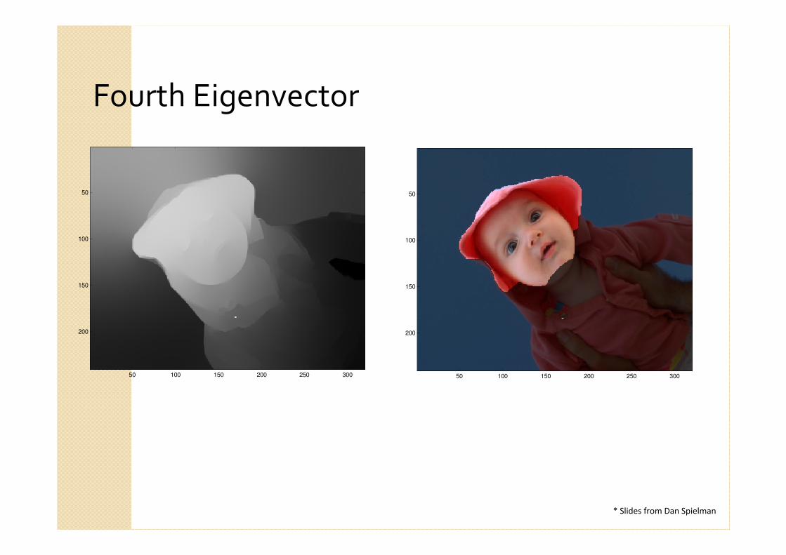
Fourth Eigenvector
50 100 150 200 250 300
50
100
150
200
50 100 150 200 250 300
50
100
150
200
* Slides from Dan Spielman
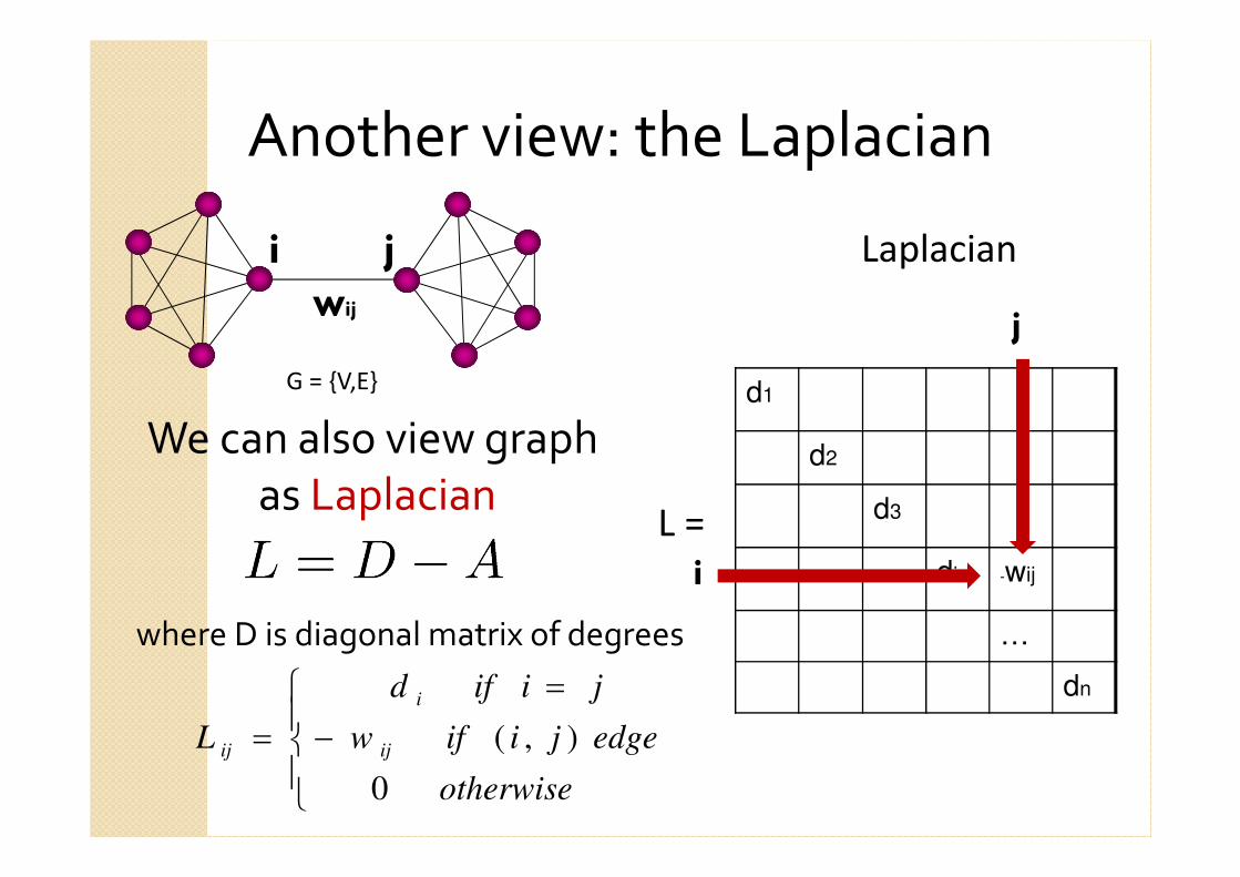
Another view: the Laplacian
where D is diagonal matrix of degrees
We can also view graph
as Laplacian
G = {V,E}
wij
i j
d1
d2
d3
di -wij
…
dn
Laplacian
j
i
L =
−
=
=
otherwise
edgejiifw
jiifd
L ij
i
ij
0
),(
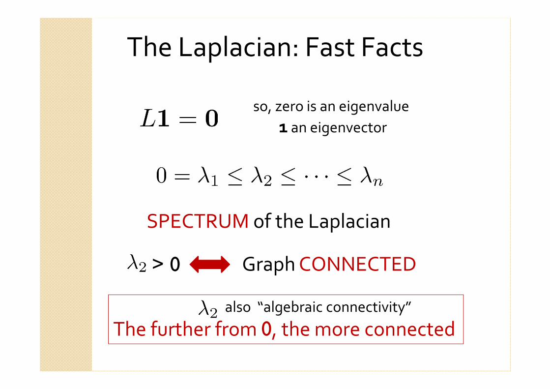
The Laplacian: Fast Facts
SPECTRUM of the Laplacian
so, zero is an eigenvalue
1 an eigenvector
> 0 Graph CONNECTED
also “algebraic connectivity”
The further from 0, the more connected
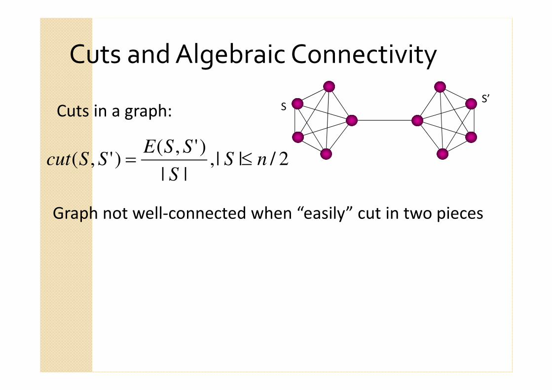
Cuts and Algebraic Connectivity
2/||,||
)',()',( nS
S
SSESScut ≤=
Cuts in a graph:
Graph not well-connected when “easily” cut in two pieces
SS’
Graph not well-connected when “easily” cut in two pieces
SS’
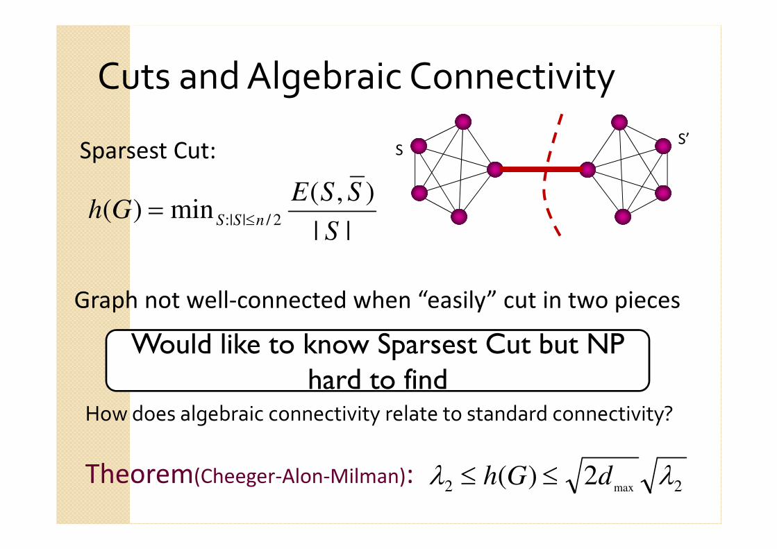
||
),(min)(
2/|:|S
SSEGh nSS ≤=
Sparsest Cut:
Would like to know Sparsest Cut but NP hard to find
How does algebraic connectivity relate to standard connectivity?
Theorem(Cheeger-Alon-Milman):22 max
2)( λλ dGh ≤≤
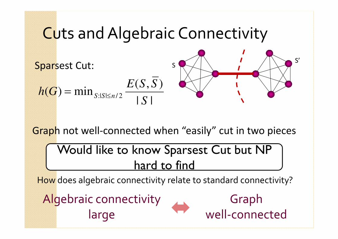
Cuts and Algebraic Connectivity
Graph not well-connected when “easily” cut in two pieces
SS’
||
),(min)( 2/|:|
S
SSEGh nSS ≤=
Sparsest Cut:
Algebraic connectivity
large
Graph
well-connected
How does algebraic connectivity relate to standard connectivity?
Would like to know Sparsest Cut but NP hard to find
Cuts and Algebraic Connectivity
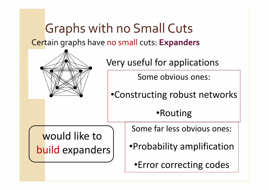
Graphs with no Small CutsCertain graphs have no small cuts: Expanders
Very useful for applications
Some obvious ones:
•Constructing robust networks
•Routing
Some far less obvious ones:
•Probability amplification
•Error correcting codes
would like to
build expanders
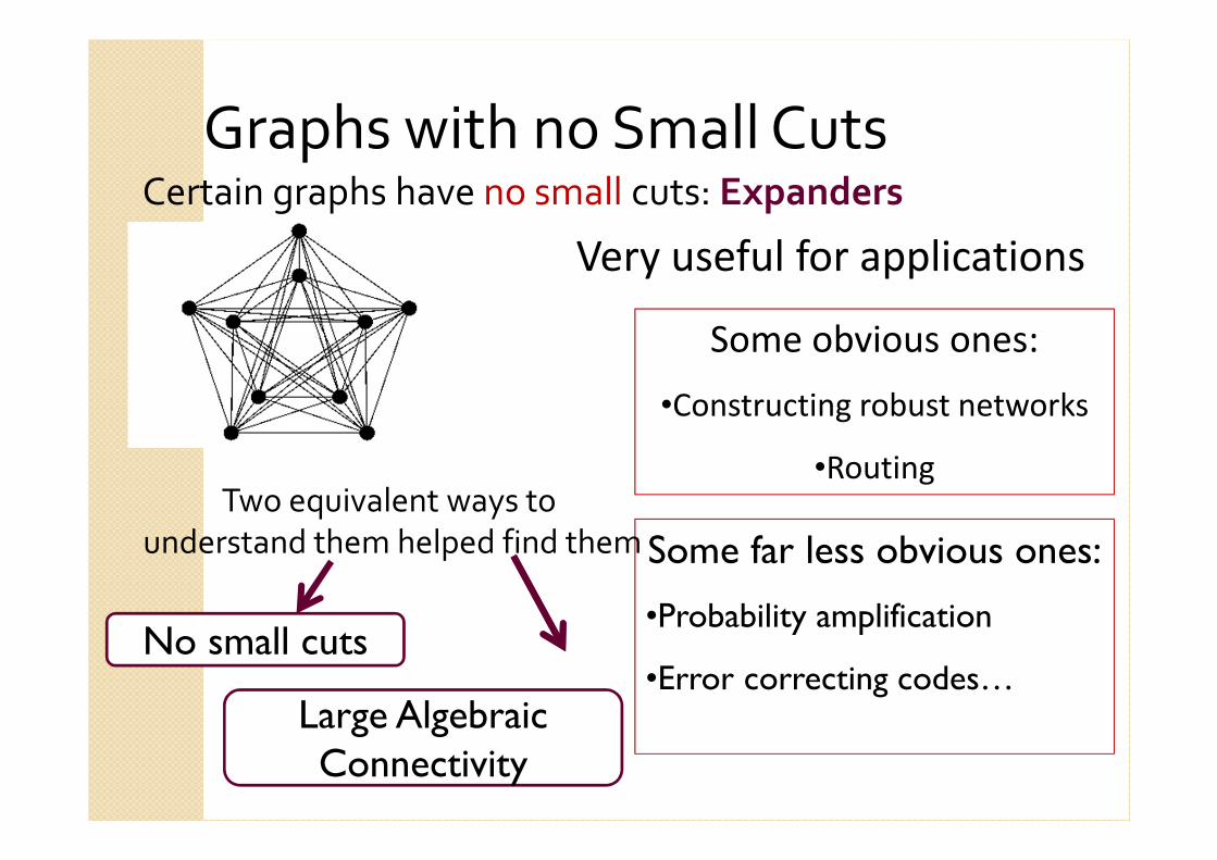
Certain graphs have no small cuts: Expanders
Very useful for applications
Some obvious ones:
•Constructing robust networks
•Routing
Some far less obvious ones:
•Probability amplification
•Error correcting codes…
Two equivalent ways to
understand them helped find them
No small cuts
Large Algebraic Connectivity
Graphs with no Small Cuts
Today
� More on evectors and evalues
� The Laplacian, revisited
� Properties of Laplacian spectra, PSD
matrices.
� Spectra of common graphs.
� Start bounding Laplacian evalues
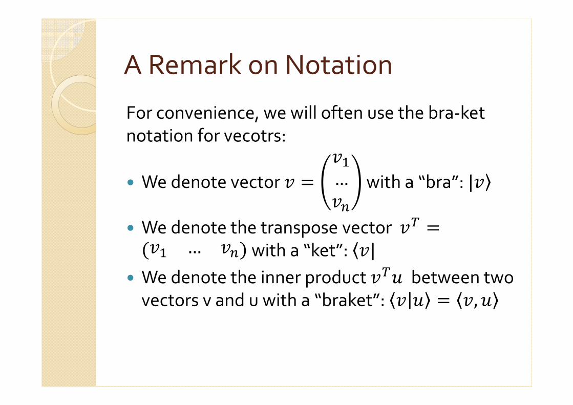
A Remark on Notation
For convenience, we will often use the bra-ket
notation for vecotrs:
� We denote vector � � ��…�� with a “bra”: |��� We denote the transpose vector �� ��� … �� with a “ket”: �|� We denote the inner product �� between two
vectors v and u with a “braket”: � � �, �
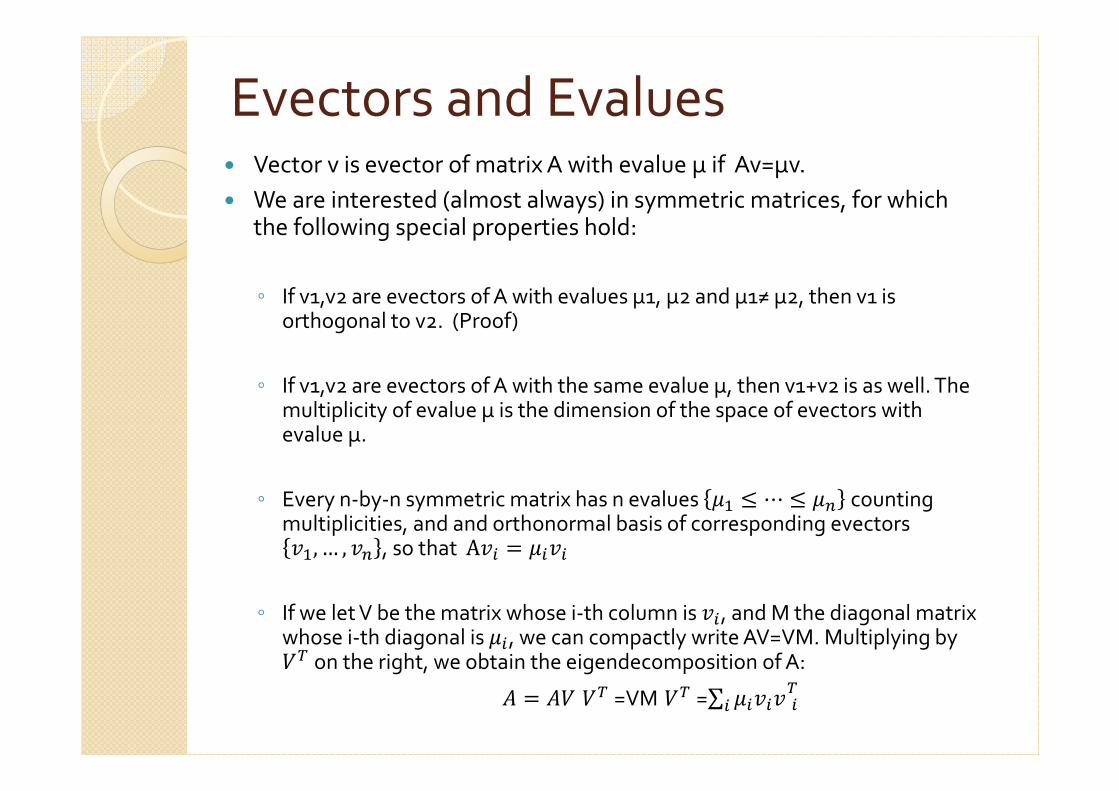
Evectors and Evalues� Vector v is evector of matrix A with evalue µ if Av=µv.
� We are interested (almost always) in symmetric matrices, for which the following special properties hold:
◦ If v1,v2 are evectors of A with evalues µ1, µ2 and µ1≠ µ2, then v1 is orthogonal to v2. (Proof)
◦ If v1,v2 are evectors of A with the same evalue µ, then v1+v2 is as well. The multiplicity of evalue µ is the dimension of the space of evectors with evalue µ.
◦ Every n-by-n symmetric matrix has n evalues � � ⋯ � � counting multiplicities, and and orthonormal basis of corresponding evectors��, … , �� , so that A�� � ���
◦ If we let V be the matrix whose i-th column is ��, and M the diagonal matrix whose i-th diagonal is �, we can compactly write AV=VM. Multiplying by ��on the right, we obtain the eigendecomposition of A:� � �� ��=VM ��=∑ ���� ���
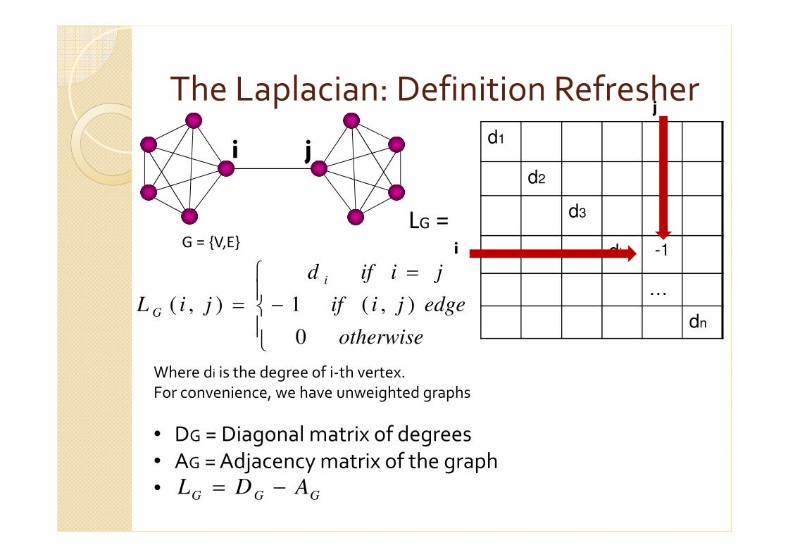
The Laplacian: Definition Refresher
G = {V,E}
i jd1
d2
d3
di -1
…
dn
j
i
LG =
Where di is the degree of i-th vertex.
For convenience, we have unweighted graphs
GGG ADL −=
• DG = Diagonal matrix of degrees
• AG = Adjacency matrix of the graph
•
−
=
=
otherwise
edgejiif
jiifd
jiL
i
G
0
),(1),(
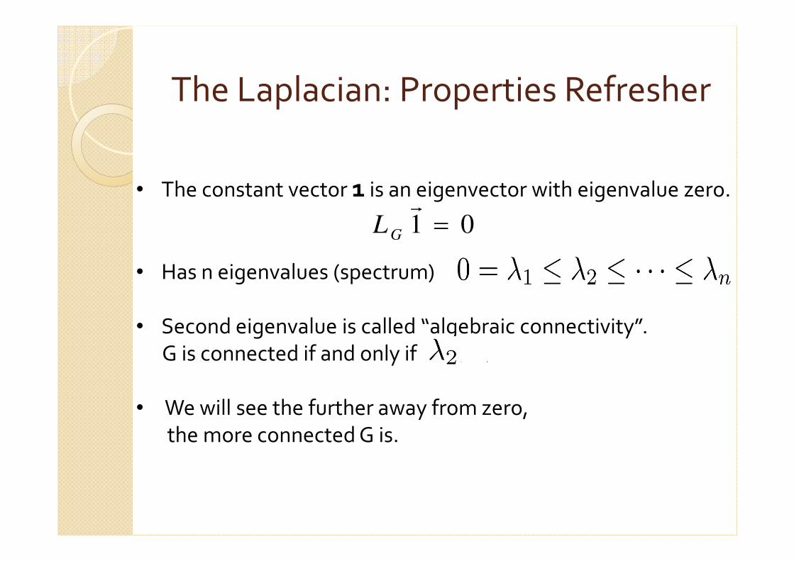
The Laplacian: Properties Refresher
• The constant vector 1 is an eigenvector with eigenvalue zero.
• Has n eigenvalues (spectrum)
• Second eigenvalue is called “algebraic connectivity”.
G is connected if and only if
• We will see the further away from zero,
the more connected G is.
> 0
01 =r
GL
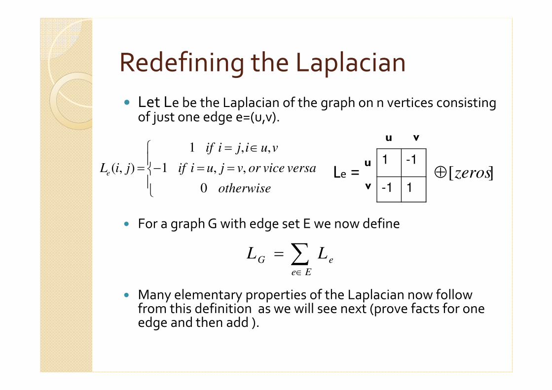
Redefining the Laplacian
� Let Le be the Laplacian of the graph on n vertices consisting of just one edge e=(u,v).
� For a graph G with edge set E we now define
� Many elementary properties of the Laplacian now follow from this definition as we will see next (prove facts for one edge and then add ).
1 -1
-1 1
uLe =
==−
∈=
=
otherwise
versaviceorvjuiif
vuijiif
jiLe
0
,,1
,,1
),(
v
u v
∑∈
=Ee
eG LL
][zeros⊕
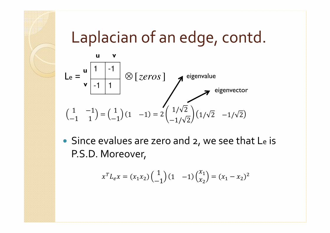
Laplacian of an edge, contd.
1 -1
-1 1
uLe =
v
u v
][zeros⊗
1 �1�1 1 � 1�1 1 �1 � 2 1/ 2�1/ 2 1/ 2 �1/ 2
eigenvalue
eigenvector
� Since evalues are zero and 2, we see that Le is
P.S.D. Moreover,
����� � ������ 1�1 1 �1 ���� � ��� � ����
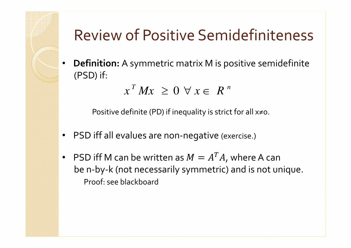
Review of Positive Semidefiniteness
• Definition: A symmetric matrix M is positive semidefinite
(PSD) if:
Positive definite (PD) if inequality is strict for all x≠0.
• PSD iff all evalues are non-negative (exercise.)
• PSD iff M can be written as � � ���, where A can be n-by-k (not necessarily symmetric) and is not unique.
Proof: see blackboard
nTRxMxx ∈∀≥ 0
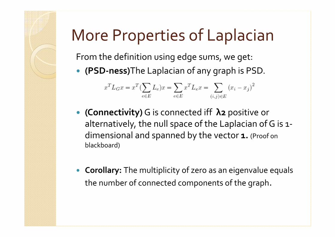
More Properties of LaplacianFrom the definition using edge sums, we get:
� (PSD-ness)The Laplacian of any graph is PSD.
� (Connectivity) G is connected iff λ2 positive or
alternatively, the null space of the Laplacian of G is 1-
dimensional and spanned by the vector 1. (Proof on
blackboard)
� Corollary: The multiplicity of zero as an eigenvalue equals
the number of connected components of the graph.
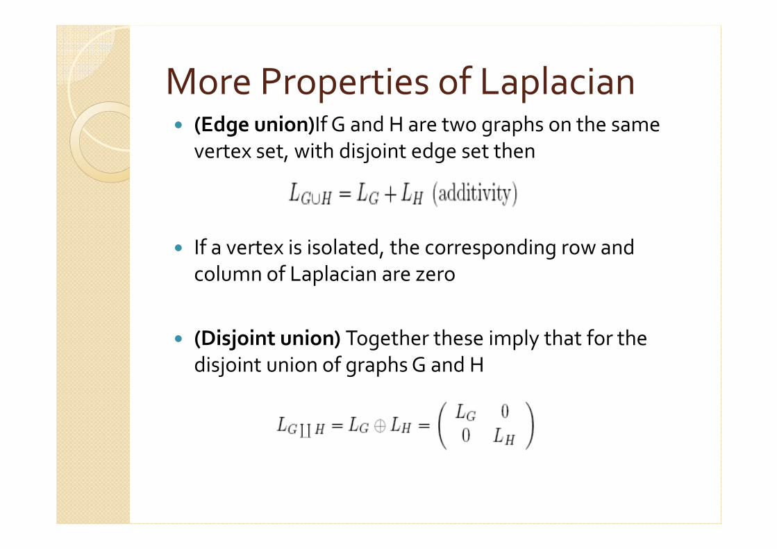
More Properties of Laplacian� (Edge union)If G and H are two graphs on the same
vertex set, with disjoint edge set then
� If a vertex is isolated, the corresponding row and
column of Laplacian are zero
� (Disjoint union) Together these imply that for the
disjoint union of graphs G and H
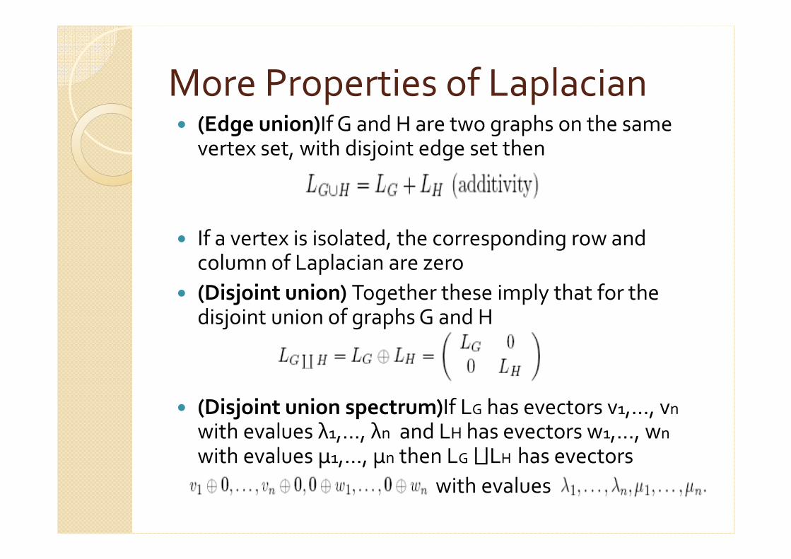
More Properties of Laplacian� (Edge union)If G and H are two graphs on the same
vertex set, with disjoint edge set then
� If a vertex is isolated, the corresponding row and column of Laplacian are zero
� (Disjoint union) Together these imply that for the disjoint union of graphs G and H
� (Disjoint union spectrum)If LG has evectors v1,…, vn
with evalues λ1,…, λn and LH has evectors w1,…, wn
with evalues µ1,…, µn then LG⨆LH has evectors
with evalues
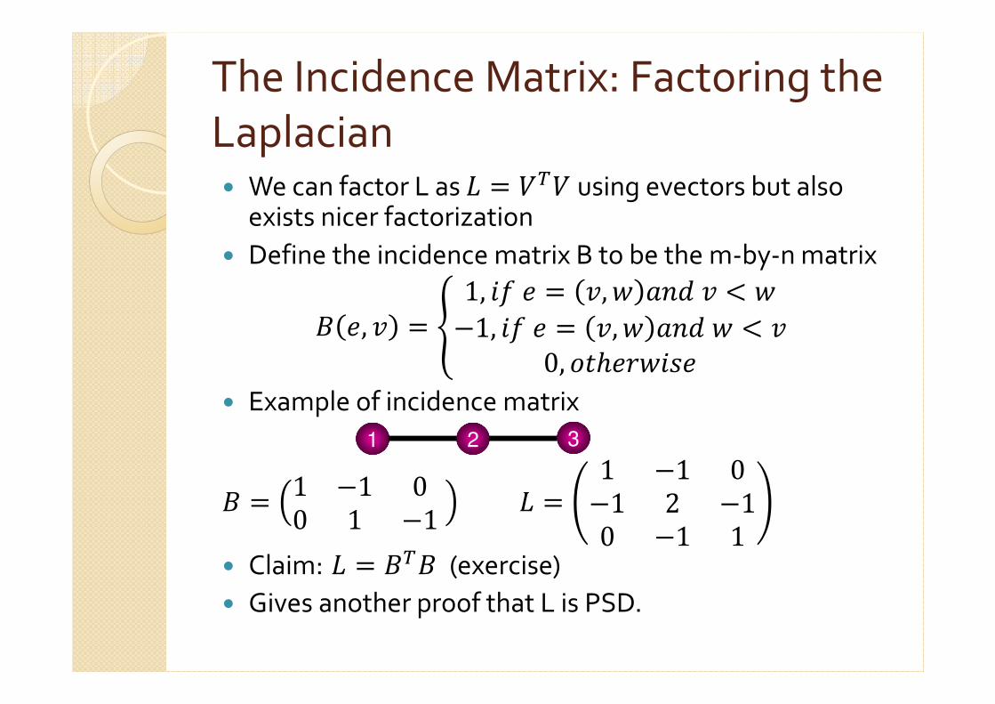
The Incidence Matrix: Factoring the
Laplacian� We can factor L as � � ���using evectors but also
exists nicer factorization
� Define the incidence matrix B to be the m-by-n matrix
! ", � � # 1, $%" � �,& '()� * &�1, $%" � �,& '()& * �0, ,-."/&$0"� Example of incidence matrix ! � 1 �1 00 1 �1 � � 1 �1 0�1 2 �10 �1 1� Claim: � � !�!(exercise)
� Gives another proof that L is PSD.
1 2 3
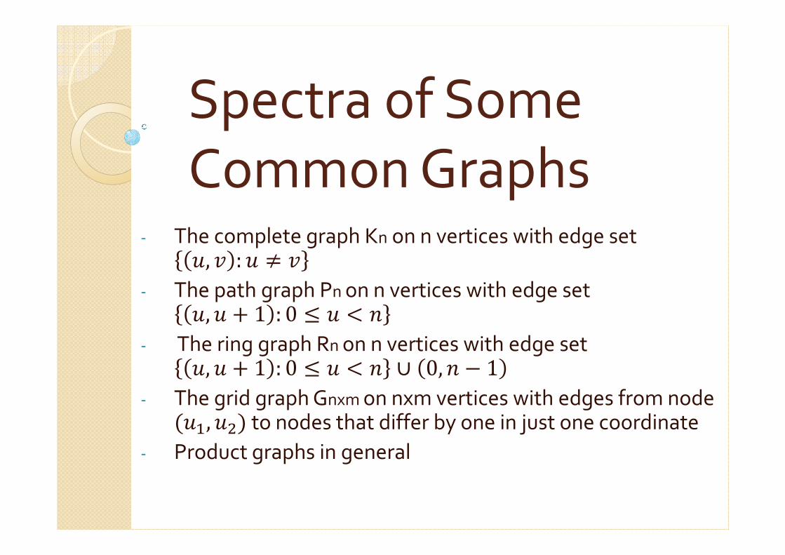
Spectra of Some
Common Graphs- The complete graph Kn on n vertices with edge set , � : 2 �- The path graph Pn on n vertices with edge set , 3 1 : 0 � * (- The ring graph Rn on n vertices with edge set , 3 1 : 0 � * ( ∪ 0, ( � 1- The grid graph Gnxm on nxm vertices with edges from node��, �� to nodes that differ by one in just one coordinate
- Product graphs in general
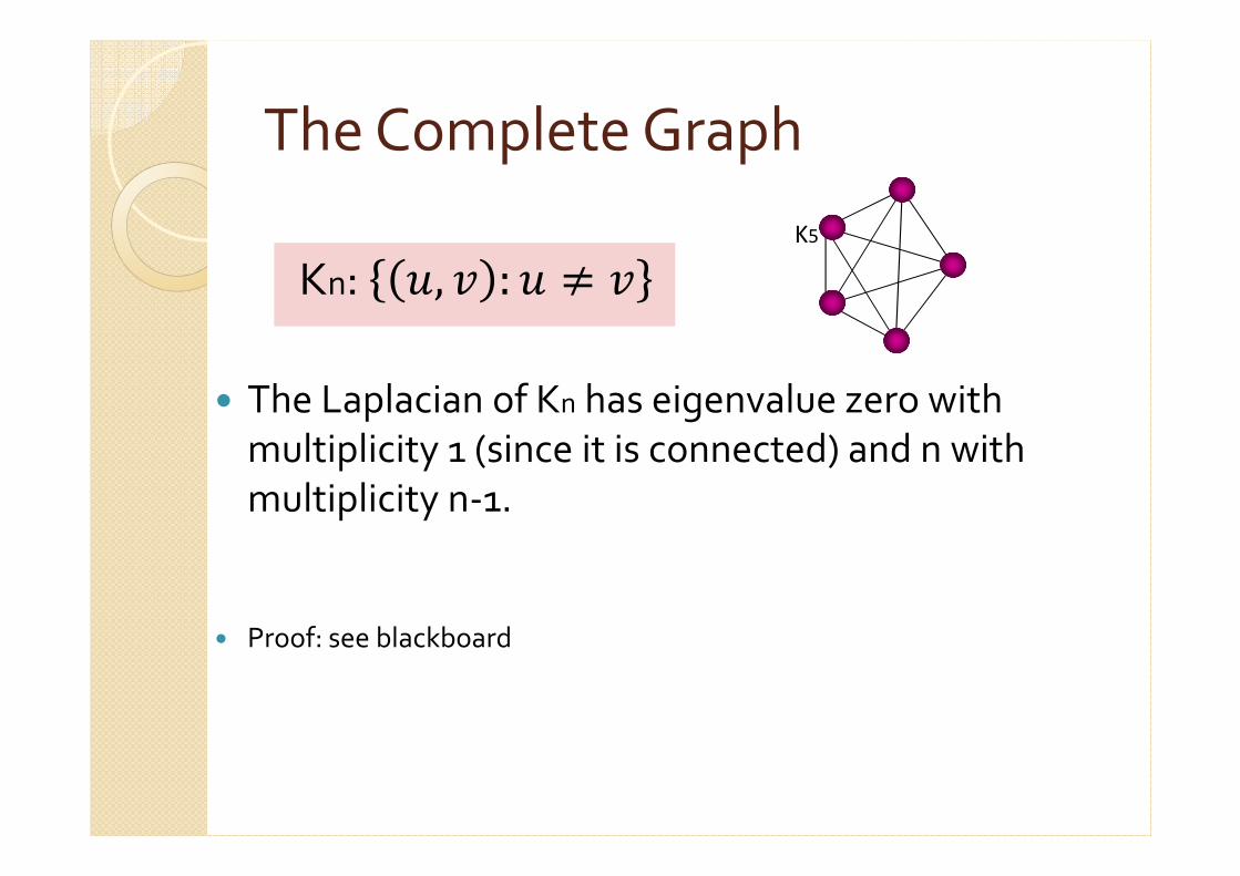
Kn: , � : 2 �� The Laplacian of Kn has eigenvalue zero with
multiplicity 1 (since it is connected) and n with
multiplicity n-1.
� Proof: see blackboard
The Complete Graph
K5
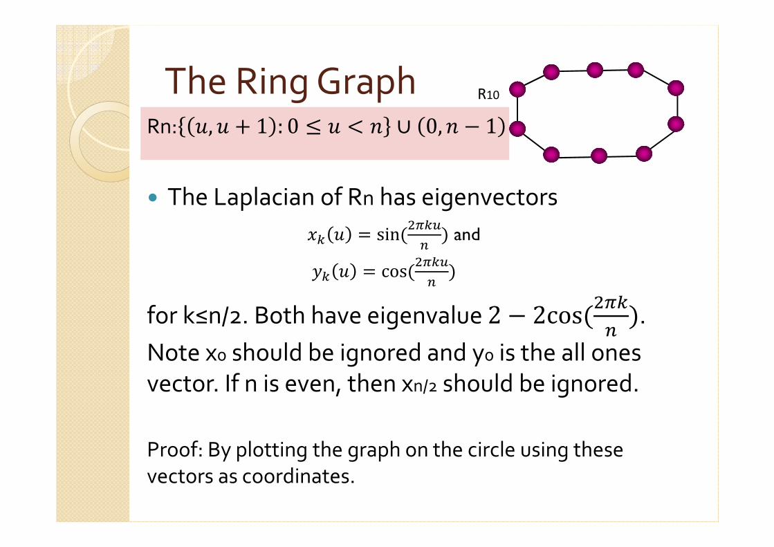
Rn: , 3 1 : 0 � * ( ∪ 0, ( � 1� The Laplacian of Rn has eigenvectors
�5 � sin��95:� � and
;5 � cos��95:� �for k≤n/2. Both have eigenvalue 2 � 2cos��95� �. Note x0 should be ignored and y0 is the all ones
vector. If n is even, then xn/2 should be ignored.
Proof: By plotting the graph on the circle using these
vectors as coordinates.
The Ring Graph R10
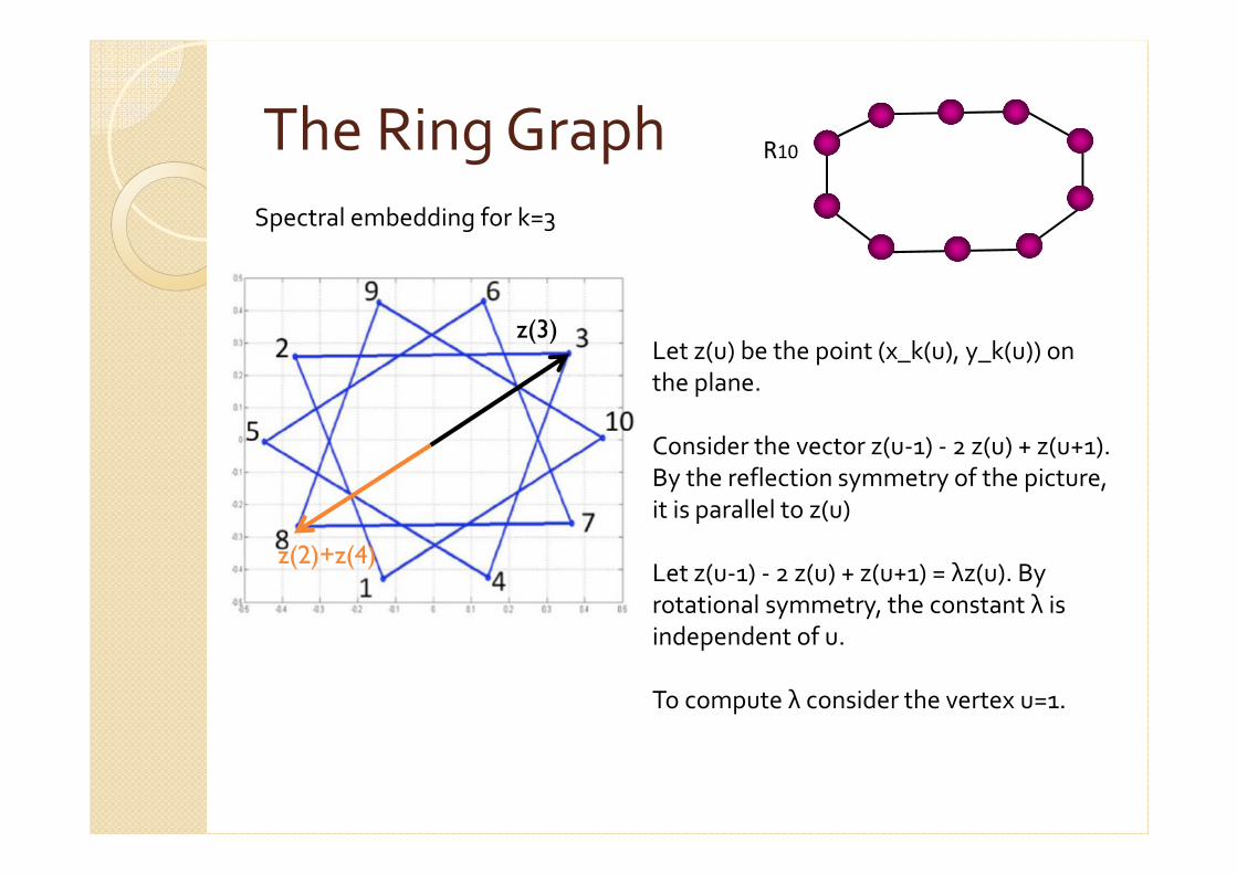
The Ring Graph
Let z(u) be the point (x_k(u), y_k(u)) on
the plane.
Consider the vector z(u-1) - 2 z(u) + z(u+1).
By the reflection symmetry of the picture,
it is parallel to z(u)
Let z(u-1) - 2 z(u) + z(u+1) = λz(u). By
rotational symmetry, the constant λ is
independent of u.
To compute λ consider the vertex u=1.
Spectral embedding for k=3
R10
z(3)
z(2)+z(4)
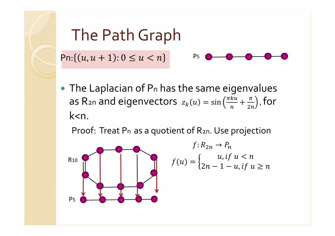
The Path GraphPn: , 3 1 : 0 � * (� The Laplacian of Pn has the same eigenvalues
as R2n and eigenvectors >5 � sin 95:� 3 9�� ,for
k<n.
Proof: Treat Pn as a quotient of R2n. Use projection%: ?�� → A�%�� � B , $% * (2( � 1 � , $% C (R10
P5
P5
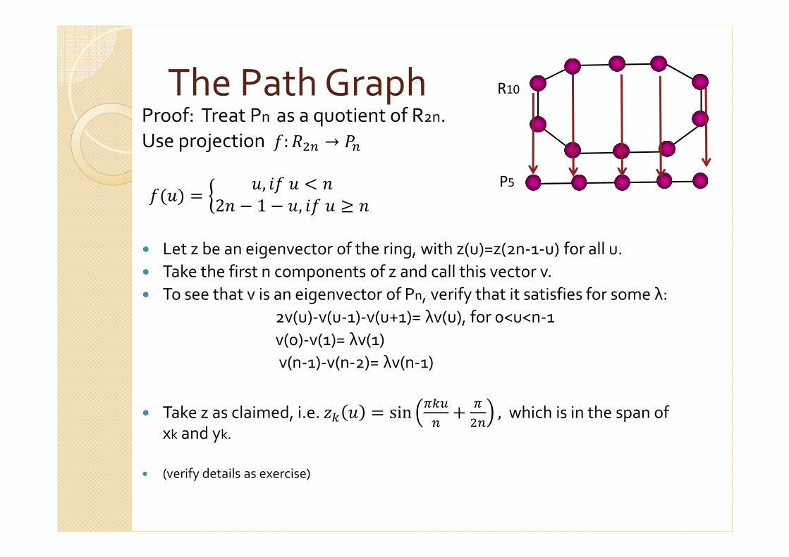
The Path GraphProof: Treat Pn as a quotient of R2n.
Use projection %: ?�� → A�%�� � B , $% * (2( � 1 � , $% C (� Let z be an eigenvector of the ring, with z(u)=z(2n-1-u) for all u.
� Take the first n components of z and call this vector v.
� To see that v is an eigenvector of Pn, verify that it satisfies for some λ:
2v(u)-v(u-1)-v(u+1)= λv(u), for 0<u<n-1
v(0)-v(1)= λv(1)
v(n-1)-v(n-2)= λv(n-1)
� Take z as claimed, i.e. >5 � sin 95:� 3 9�� ,which is in the span of xk and yk.
� (verify details as exercise)
R10
P5
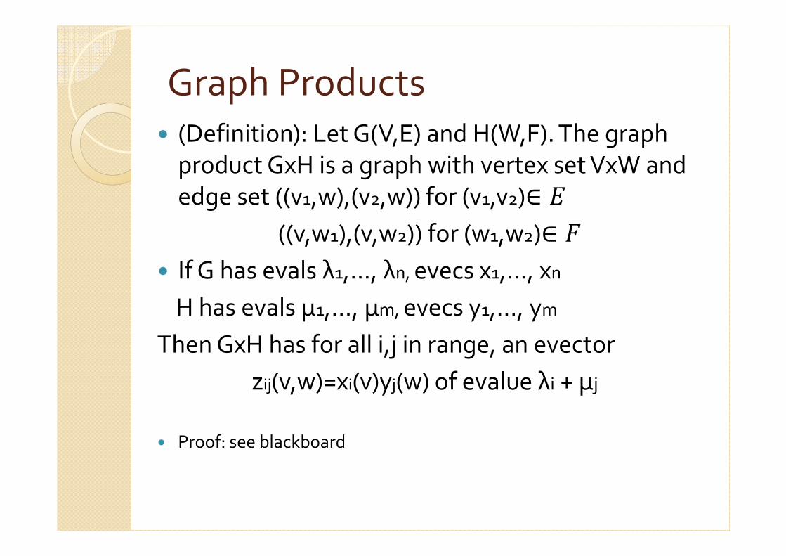
Graph Products� (Definition): Let G(V,E) and H(W,F). The graph
product GxH is a graph with vertex set VxW and
edge set ((v1,w),(v2,w)) for (v1,v2)∈ E((v,w1),(v,w2)) for (w1,w2)∈ F
� If G has evals λ1,…, λn, evecs x1,…, xn
H has evals µ1,…, µm, evecs y1,…, ym
Then GxH has for all i,j in range, an evector
zij(v,w)=xi(v)yj(w) of evalue λi + µj
� Proof: see blackboard
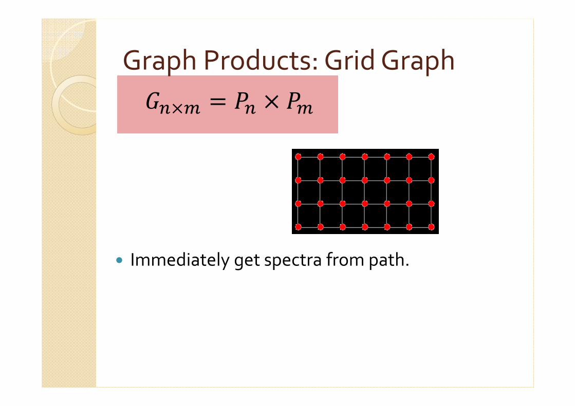
Graph Products: Grid Graph
� Immediately get spectra from path.
G�HI � A� H AI
Start Bounding
Laplacian Eigenvalues
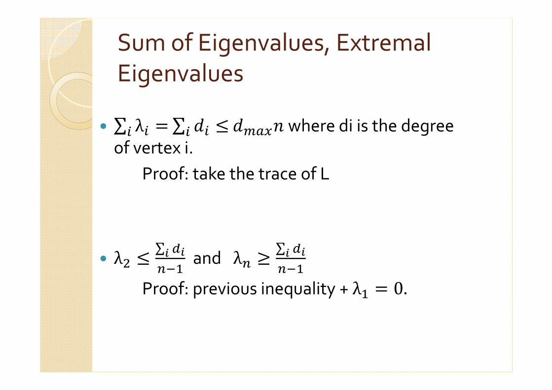
Sum of Eigenvalues, Extremal
Eigenvalues
� ∑ λ� �� ∑ )� �� )IKL( where di is the degree
of vertex i.
Proof: take the trace of L
� λ� � ∑ MNN�O� and λ� C ∑ MNN�O� Proof: previous inequality + λ� � 0.
Courant-Fischer
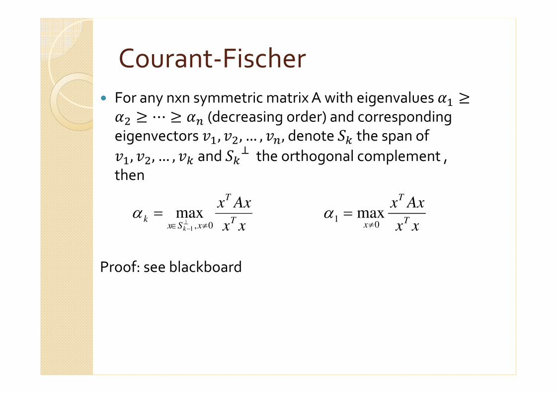
� For any nxn symmetric matrix A with eigenvalues Q� CQ� C ⋯ C Q� (decreasing order) and corresponding
eigenvectors ��, ��, … , ��, denote R5 the span of ��, ��, … , �5 and R5S the orthogonal complement , then
Proof: see blackboard
xx
AxxT
T
xSxk
k 0,1
max≠∈ ⊥
−
=αxx
AxxT
T
x 01 max
≠=α
Courant-Fischer
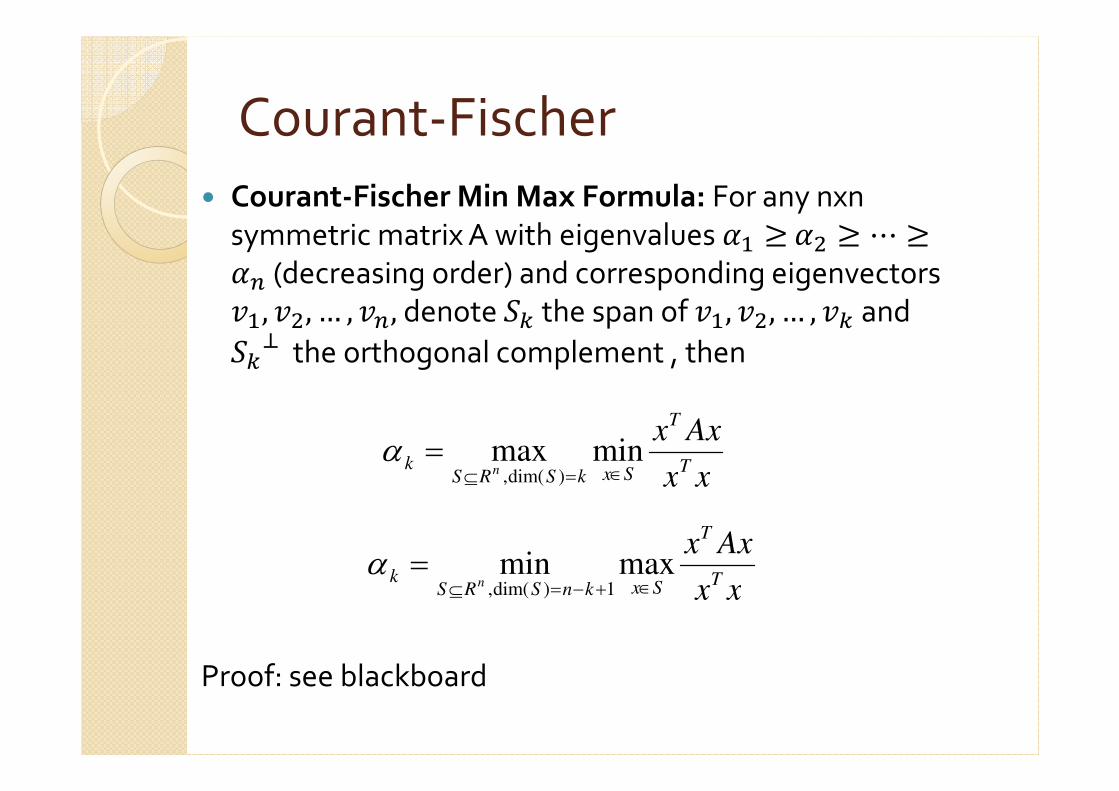
� Courant-Fischer Min Max Formula: For any nxn
symmetric matrix A with eigenvalues Q� CQ� C ⋯ CQ� (decreasing order) and corresponding eigenvectors ��, ��, … , ��, denote R5 the span of ��, ��, … , �5 and R5S the orthogonal complement , then
Proof: see blackboard
xx
AxxT
T
SxknSRSk n ∈+−=⊆= maxmin
1)dim(,
α
xx
AxxT
T
SxkSRSk n ∈=⊆= minmax
)dim(,
α
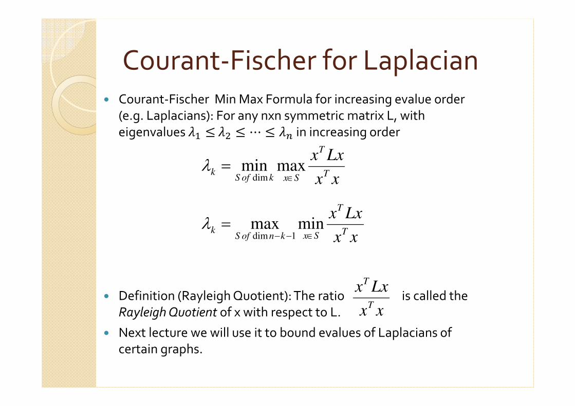
Courant-Fischer for Laplacian� Courant-Fischer Min Max Formula for increasing evalue order
(e.g. Laplacians): For any nxn symmetric matrix L, with
eigenvalues T� � T� � ⋯ � T� in increasing order
� Definition (Rayleigh Quotient): The ratio is called the
Rayleigh Quotient of x with respect to L.
� Next lecture we will use it to bound evalues of Laplacians of
certain graphs.
xx
LxxT
T
SxkofSk
∈= maxmin
dimλ
xx
LxxT
T
SxknofSk ∈−−= minmax
1dimλ
xx
LxxT
T