Embed Size (px)
Citation preview

CS 561, Sessions 8-9 1
Administrativia
• Assignment 1 due tuesday 9/24/2002 BEFORE midnight
• Midterm exam 10/10/2002
CS 561, Sessions 8-9 2
Last time: search strategies
Uninformed: Use only information available in the problem formulation• Breadth-first• Uniform-cost• Depth-first• Depth-limited• Iterative deepening
Informed: Use heuristics to guide the search• Best first:• Greedy search – queue first nodes that maximize heuristic “desirability”
based on estimated path cost from current node to goal;• A* search – queue first nodes that maximize sum of path cost so far and
estimated path cost to goal.• Iterative improvement – keep no memory of path; work on a single current
state and iteratively improve its “value.”• Hill climbing – select as new current state the successor state which
maximizes value.• Simulated annealing – refinement on hill climbing by which “bad moves”
are permitted, but with decreasing size and frequency. Will find global extremum.

CS 561, Sessions 8-9 3
Exercise: Search Algorithms
The following figure shows a portion of a partially expanded search tree. Each arc between nodes is labeled with the cost of the corresponding operator, and the leaves are labeled with the value of the heuristic function, h.
Which node (use the node’s letter) will be expanded next by each of the following search algorithms?
(a) Depth-first search(b) Breadth-first search(c) Uniform-cost search(d) Greedy search
(e) A* search
5
D
5
A
C
54
19
6
3
h=15
B
F GE
h=8h=12h=10 h=10
h=18
H
h=20
h=14

CS 561, Sessions 8-9 4
Depth-first search
Node queue: initialization
# state depth path cost parent #
1 A 0 0 --

CS 561, Sessions 8-9 5
Depth-first search
Node queue: add successors to queue front; empty queue from top
# state depth path cost parent #
2 B 1 3 13 C 1 19 14 D 1 5 11 A 0 0 --

CS 561, Sessions 8-9 6
Depth-first search
Node queue: add successors to queue front; empty queue from top
# state depth path cost parent #
5 E 2 7 26 F 2 8 27 G 2 8 28 H 2 9 22 B 1 3 13 C 1 19 14 D 1 5 11 A 0 0 --

CS 561, Sessions 8-9 7
Depth-first search
Node queue: add successors to queue front; empty queue from top
# state depth path cost parent #
5 E 2 7 26 F 2 8 27 G 2 8 28 H 2 9 22 B 1 3 13 C 1 19 14 D 1 5 11 A 0 0 --

CS 561, Sessions 8-9 8
Exercise: Search Algorithms
The following figure shows a portion of a partially expanded search tree. Each arc between nodes is labeled with the cost of the corresponding operator, and the leaves are labeled with the value of the heuristic function, h.
Which node (use the node’s letter) will be expanded next by each of the following search algorithms?
(a) Depth-first search(b) Breadth-first search(c) Uniform-cost search(d) Greedy search
(e) A* search
5
D
5
A
C
54
19
6
3
h=15
B
F GE
h=8h=12h=10 h=10
h=18
H
h=20
h=14

CS 561, Sessions 8-9 9
Breadth-first search
Node queue: initialization
# state depth path cost parent #
1 A 0 0 --

CS 561, Sessions 8-9 10
Breadth-first search
Node queue: add successors to queue end; empty queue from top
# state depth path cost parent #
1 A 0 0 --2 B 1 3 13 C 1 19 14 D 1 5 1

CS 561, Sessions 8-9 11
Breadth-first search
Node queue: add successors to queue end; empty queue from top
# state depth path cost parent #
1 A 0 0 --2 B 1 3 13 C 1 19 14 D 1 5 15 E 2 7 26 F 2 8 27 G 2 8 28 H 2 9 2

CS 561, Sessions 8-9 12
Breadth-first search
Node queue: add successors to queue end; empty queue from top
# state depth path cost parent #
1 A 0 0 --2 B 1 3 13 C 1 19 14 D 1 5 15 E 2 7 26 F 2 8 27 G 2 8 28 H 2 9 2

CS 561, Sessions 8-9 13
Exercise: Search Algorithms
The following figure shows a portion of a partially expanded search tree. Each arc between nodes is labeled with the cost of the corresponding operator, and the leaves are labeled with the value of the heuristic function, h.
Which node (use the node’s letter) will be expanded next by each of the following search algorithms?
(a) Depth-first search(b) Breadth-first search(c) Uniform-cost search(d) Greedy search
(e) A* search
5
D
5
A
C
54
19
6
3
h=15
B
F GE
h=8h=12h=10 h=10
h=18
H
h=20
h=14

CS 561, Sessions 8-9 14
Uniform-cost search
Node queue: initialization
# state depth path cost parent #
1 A 0 0 --

CS 561, Sessions 8-9 15
Uniform-cost search
Node queue: add successors to queue so that entire queue is sorted by path cost so far; empty queue from top
# state depth path cost parent #
1 A 0 0 --2 B 1 3 13 D 1 5 14 C 1 19 1

CS 561, Sessions 8-9 16
Uniform-cost search
Node queue: add successors to queue so that entire queue is sorted by path cost so far; empty queue from top
# state depth path cost parent #
1 A 0 0 --2 B 1 3 13 D 1 5 15 E 2 7 26 F 2 8 27 G 2 8 28 H 2 9 24 C 1 19 1

CS 561, Sessions 8-9 17
Uniform-cost search
Node queue: add successors to queue so that entire queue is sorted by path cost so far; empty queue from top
# state depth path cost parent #
1 A 0 0 --2 B 1 3 13 D 1 5 15 E 2 7 26 F 2 8 27 G 2 8 28 H 2 9 24 C 1 19 1

CS 561, Sessions 8-9 18
Exercise: Search Algorithms
The following figure shows a portion of a partially expanded search tree. Each arc between nodes is labeled with the cost of the corresponding operator, and the leaves are labeled with the value of the heuristic function, h.
Which node (use the node’s letter) will be expanded next by each of the following search algorithms?
(a) Depth-first search(b) Breadth-first search(c) Uniform-cost search(d) Greedy search
(e) A* search
5
D
5
A
C
54
19
6
3
h=15
B
F GE
h=8h=12h=10 h=10
h=18
H
h=20
h=14

CS 561, Sessions 8-9 19
Greedy search
Node queue: initialization
# state depth path cost total parent #cost to goalcost
1 A 0 0 20 20 --

CS 561, Sessions 8-9 20
Greedy search
Node queue: Add successors to queue, sorted by cost to goal.
# state depth path cost total parent #cost to goalcost
1 A 0 0 20 20 --2 B 1 3 14 17 13 D 1 5 15 20 14 C 1 19 18 37 1
Sort key

CS 561, Sessions 8-9 21
Greedy search
Node queue: Add successors to queue, sorted by cost to goal.
# state depth path cost total parent #cost to goalcost
1 A 0 0 20 20 --2 B 1 3 14 17 15 G 2 8 8 16 27 E 2 7 10 17 26 H 2 9 10 19 28 F 2 8 12 20 23 D 1 5 15 20 14 C 1 19 18 37 1

CS 561, Sessions 8-9 22
Greedy search
Node queue: Add successors to queue, sorted by cost to goal.
# state depth path cost total parent #cost to goalcost
1 A 0 0 20 20 --2 B 1 3 14 17 15 G 2 8 8 16 27 E 2 7 10 17 26 H 2 9 10 19 28 F 2 8 12 20 23 D 1 5 15 20 14 C 1 19 18 37 1

CS 561, Sessions 8-9 23
Exercise: Search Algorithms
The following figure shows a portion of a partially expanded search tree. Each arc between nodes is labeled with the cost of the corresponding operator, and the leaves are labeled with the value of the heuristic function, h.
Which node (use the node’s letter) will be expanded next by each of the following search algorithms?
(a) Depth-first search(b) Breadth-first search(c) Uniform-cost search(d) Greedy search
(e) A* search
5
D
5
A
C
54
19
6
3
h=15
B
F GE
h=8h=12h=10 h=10
h=18
H
h=20
h=14

CS 561, Sessions 8-9 24
A* search
Node queue: initialization
# state depth path cost total parent #cost to goalcost
1 A 0 0 20 20 --

CS 561, Sessions 8-9 25
A* search
Node queue: Add successors to queue, sorted by total cost.
# state depth path cost total parent #cost to goalcost
1 A 0 0 20 20 --2 B 1 3 14 17 13 D 1 5 15 20 14 C 1 19 18 37 1
Sort key

CS 561, Sessions 8-9 26
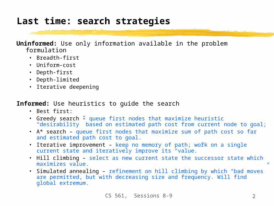
A* search
Node queue: Add successors to queue front, sorted by total cost.
# state depth path cost total parent #cost to goalcost
1 A 0 0 20 20 --2 B 1 3 14 17 15 G 2 8 8 16 26 E 2 7 10 17 27 H 2 9 10 19 23 D 1 5 15 20 18 F 2 8 12 20 24 C 1 19 18 37 1
CS 561, Sessions 8-9 27
A* search
Node queue: Add successors to queue front, sorted by total cost.
# state depth path cost total parent #cost to goalcost
1 A 0 0 20 20 --2 B 1 3 14 17 15 G 2 8 8 16 26 E 2 7 10 17 27 H 2 9 10 19 23 D 1 5 15 20 18 F 2 8 12 20 24 C 1 19 18 37 1

CS 561, Sessions 8-9 28
Exercise: Search Algorithms
The following figure shows a portion of a partially expanded search tree. Each arc between nodes is labeled with the cost of the corresponding operator, and the leaves are labeled with the value of the heuristic function, h.
Which node (use the node’s letter) will be expanded next by each of the following search algorithms?
(a) Depth-first search(b) Breadth-first search(c) Uniform-cost search(d) Greedy search
(e) A* search
5
D
5
A
C
54
19
6
3
h=15
B
F GE
h=8h=12h=10 h=10
h=18
H
h=20
h=14

CS 561, Sessions 8-9 29
Last time: Simulated annealing algorithm
• Idea: Escape local extrema by allowing “bad moves,” but gradually decrease their size and frequency.
Note: goal here is tomaximize E.-

CS 561, Sessions 8-9 30
Last time: Simulated annealing algorithm
• Idea: Escape local extrema by allowing “bad moves,” but gradually decrease their size and frequency.
Algorithm when goalis to minimize E.< -
-

CS 561, Sessions 8-9 31
This time: Outline
• Game playing• The minimax algorithm• Resource limitations• alpha-beta pruning• Elements of chance

CS 561, Sessions 8-9 32
What kind of games?
• Abstraction: To describe a game we must capture every relevant aspect of the game. Such as:• Chess• Tic-tac-toe• …
• Accessible environments: Such games are characterized by perfect information
• Search: game-playing then consists of a search through possible game positions
• Unpredictable opponent: introduces uncertainty thus game-playing must deal with contingency problems

CS 561, Sessions 8-9 33
Searching for the next move
• Complexity: many games have a huge search space• Chess: b = 35, m=100 nodes = 100 35
if each node takes about 1 ns to explorethen each move will take about 10 50 millennia
to calculate.
• Resource (e.g., time, memory) limit: optimal solution not feasible/possible, thus must approximate
1. Pruning: makes the search more efficient by discarding portions of the search tree that cannot improve quality result.
2. Evaluation functions: heuristics to evaluate utility of a state without exhaustive search.

CS 561, Sessions 8-9 34
Two-player games
• A game formulated as a search problem:
• Initial state: ?• Operators: ?• Terminal state: ?• Utility function: ?

CS 561, Sessions 8-9 35
Two-player games
• A game formulated as a search problem:
• Initial state: board position and turn• Operators: definition of legal moves• Terminal state: conditions for when game is over• Utility function: a numeric value that describes the
outcome of thegame. E.g., -1, 0, 1 for loss, draw, win.(AKA payoff function)

CS 561, Sessions 8-9 36
Game vs. search problem

CS 561, Sessions 8-9 37
Example: Tic-Tac-Toe

CS 561, Sessions 8-9 38
Type of games
CS 561, Sessions 8-9 39
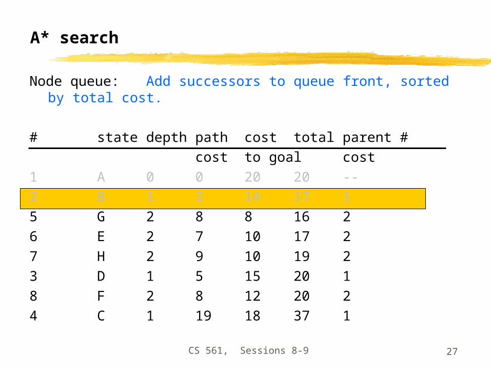
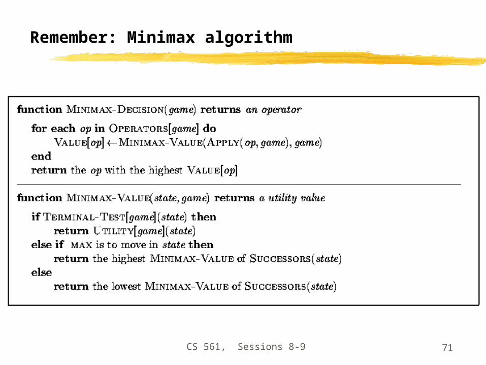
The minimax algorithm
• Perfect play for deterministic environments with perfect information
• Basic idea: choose move with highest minimax value= best achievable payoff against best play
• Algorithm: 1. Generate game tree completely2. Determine utility of each terminal state3. Propagate the utility values upward in the three by applying
MIN and MAX operators on the nodes in the current level4. At the root node use minimax decision to select the move
with the max (of the min) utility value
• Steps 2 and 3 in the algorithm assume that the opponent will play perfectly.

CS 561, Sessions 8-9 40
minimax = maximum of the minimum
1st ply
2nd ply
CS 561, Sessions 8-9 41
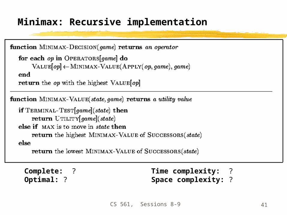
Minimax: Recursive implementation
Complete: ?Optimal: ?
Time complexity: ?Space complexity: ?

CS 561, Sessions 8-9 42
Minimax: Recursive implementation
Complete: Yes, for finite state-spaceOptimal: Yes
Time complexity: O(bm)Space complexity: O(bm) (= DFSDoes not keep all nodes in memory.)

CS 561, Sessions 8-9 43
1. Move evaluation without complete search
• Complete search is too complex and impractical
• Evaluation function: evaluates value of state using heuristics and cuts off search
• New MINIMAX:• CUTOFF-TEST: cutoff test to replace the termination condition
(e.g., deadline, depth-limit, etc.)• EVAL: evaluation function to replace utility function (e.g.,
number of chess pieces taken)

CS 561, Sessions 8-9 44
Evaluation functions
• Weighted linear evaluation function: to combine n heuristics
f = w1f1 + w2f2 + … + wnfn
E.g, w’s could be the values of pieces (1 for prawn, 3 for bishop etc.)f’s could be the number of type of pieces on the board

CS 561, Sessions 8-9 45
Note: exact values do not matter

CS 561, Sessions 8-9 46
Minimax with cutoff: viable algorithm?
Assume we have 100 seconds, evaluate 104 nodes/s;can evaluate 106 nodes/move

CS 561, Sessions 8-9 47
2. - pruning: search cutoff
• Pruning: eliminating a branch of the search tree from consideration without exhaustive examination of each node
- pruning: the basic idea is to prune portions of the search tree that cannot improve the utility value of the max or min node, by just considering the values of nodes seen so far.
• Does it work? Yes, in roughly cuts the branching factor from b to b resulting in double as far look-ahead than pure minimax

CS 561, Sessions 8-9 48
- pruning: example
6
6
MAX
6 12 8
MIN

CS 561, Sessions 8-9 49
- pruning: example
6
6
MAX
6 12 8 2
2MIN
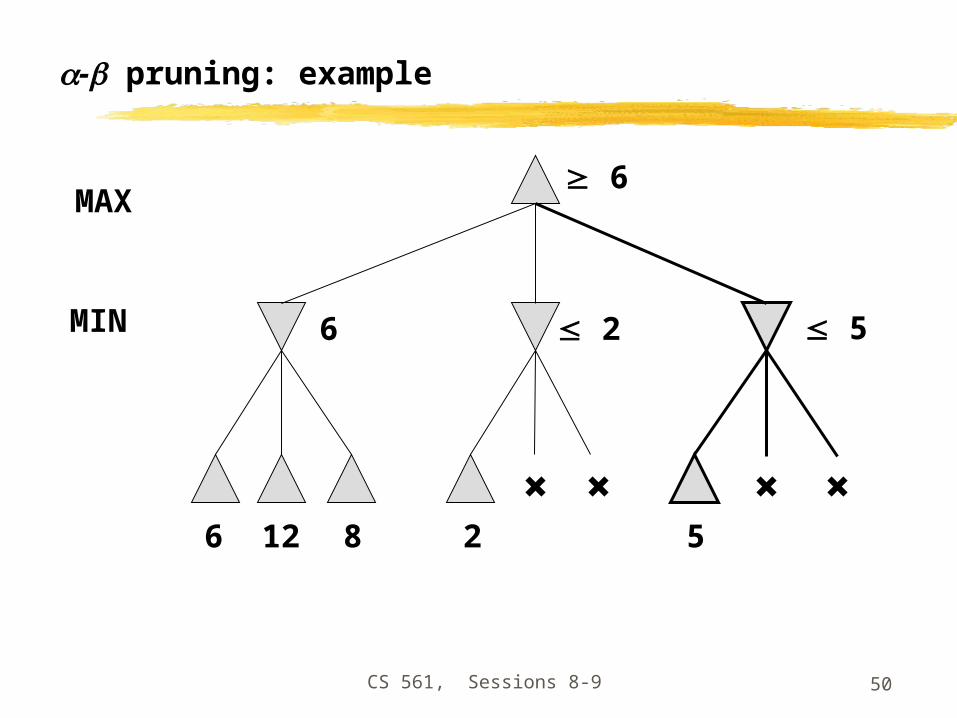
CS 561, Sessions 8-9 50
- pruning: example
6
6
MAX
6 12 8 2
2
5
5MIN

CS 561, Sessions 8-9 51
- pruning: example
6
6
MAX
6 12 8 2
2
5
5MIN
Selected move
CS 561, Sessions 8-9 52
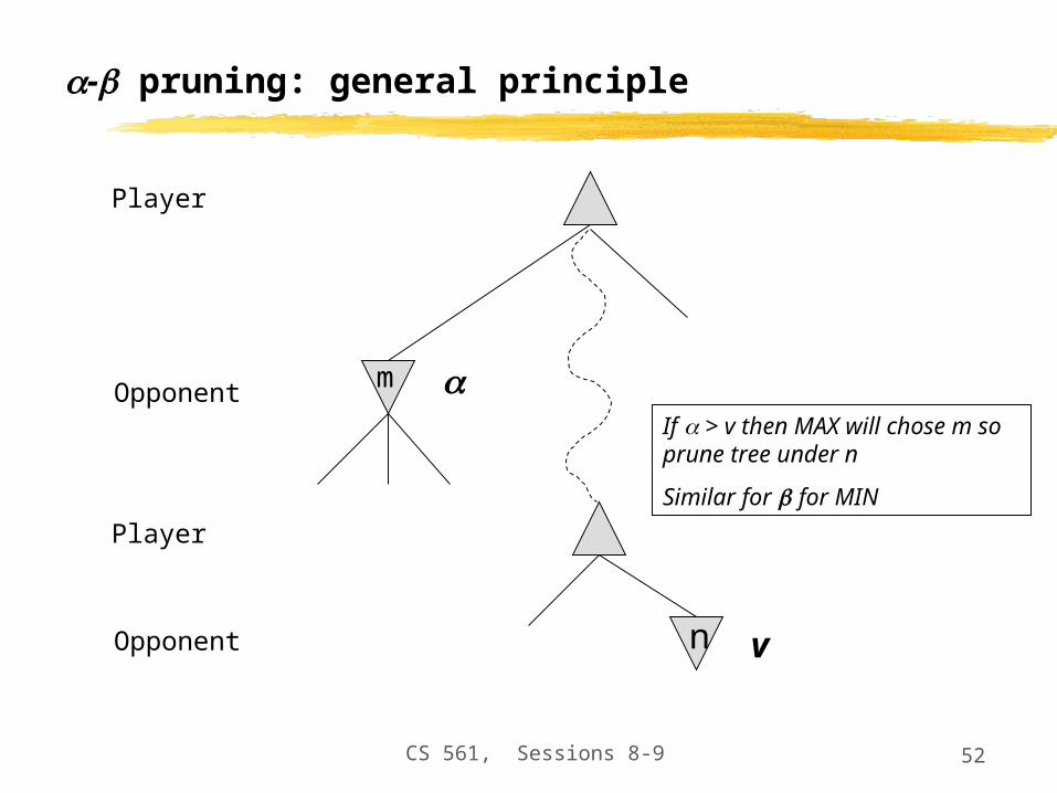
- pruning: general principle
Player
Player
Opponent
Opponent
m
n
v
If > v then MAX will chose m so prune tree under n
Similar for for MIN

CS 561, Sessions 8-9 53
Properties of -

CS 561, Sessions 8-9 54
The - algorithm

CS 561, Sessions 8-9 55
More on the - algorithm
• Same basic idea as minimax, but prune (cut away) branches of the tree that we know will not contain the solution.

CS 561, Sessions 8-9 56
More on the - algorithm: start from Minimax

CS 561, Sessions 8-9 57
Remember: Minimax: Recursive implementation
Complete: Yes, for finite state-spaceOptimal: Yes
Time complexity: O(bm)Space complexity: O(bm) (= DFSDoes not keep all nodes in memory.)

CS 561, Sessions 8-9 58
More on the - algorithm
• Same basic idea as minimax, but prune (cut away) branches of the tree that we know will not contain the solution.
• Because minimax is depth-first, let’s consider nodes along a given path in the tree. Then, as we go along this path, we keep track of: : Best choice so far for MAX : Best choice so far for MIN

CS 561, Sessions 8-9 59
More on the - algorithm: start from Minimax
Note: These are bothLocal variables. At theStart of the algorithm,We initialize them to = - and = +

CS 561, Sessions 8-9 60
More on the - algorithm
…
MAX
MIN
MAX
= - = +
5 10 6 2 8 7
Min-Value loopsover these
In Min-Value:
= - = 5
= - = 5
= - = 5
Max-Value loopsover these

CS 561, Sessions 8-9 61
More on the - algorithm
…
MAX
MIN
MAX
= - = +
5 10 6 2 8 7
In Max-Value:
= - = 5
= - = 5
= - = 5
= 5 = +Max-Value loops
over these
CS 561, Sessions 8-9 62
In Min-Value:More on the - algorithm
…
MAX
MIN
MAX
= - = +
5 10 6 2 8 7 = - = 5
= - = 5
= - = 5
= 5 = +
= 5 = 2End loop and return 5
Min-Value loopsover these

CS 561, Sessions 8-9 63
In Max-Value:More on the - algorithm
…
MAX
MIN
MAX
= - = +
5 10 6 2 8 7 = - = 5
= - = 5
= - = 5
= 5 = +
= 5 = 2End loop and return 5
= 5 = +
Max-Value loopsover these

CS 561, Sessions 8-9 64
Another way to understand the algorithm
• From: http://yoda.cis.temple.edu:8080/UGAIWWW/lectures95/search/alpha-beta.html
• For a given node N,
is the value of N to MAX is the value of N to MIN

CS 561, Sessions 8-9 65
Example

CS 561, Sessions 8-9 66
- algorithm:
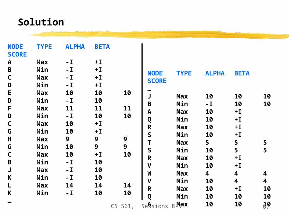
CS 561, Sessions 8-9 67
Solution
NODE TYPE ALPHA BETA SCORE A Max -I +IB Min -I +I C Max -I +I D Min -I +I E Max 10 10 10 D Min -I 10 F Max 11 11 11 D Min -I 10 10 C Max 10 +I G Min 10 +I H Max 9 9 9 G Min 10 9 9 C Max 10 +I 10 B Min -I 10 J Max -I 10 K Min -I 10 L Max 14 14 14 K Min -I 10 10 …
NODE TYPE ALPHA BETA SCORE …J Max 10 10 10 B Min -I 10 10 A Max 10 +I Q Min 10 +I R Max 10 +I S Min 10 +I T Max 5 5 5 S Min 10 5 5 R Max 10 +I V Min 10 +I W Max 4 4 4 V Min 10 4 4 R Max 10 +I 10 Q Min 10 10 10 A Max 10 10 10

CS 561, Sessions 8-9 68
State-of-the-art for deterministic games

CS 561, Sessions 8-9 69
Nondeterministic games

CS 561, Sessions 8-9 70
Algorithm for nondeterministic games
CS 561, Sessions 8-9 71
Remember: Minimax algorithm

CS 561, Sessions 8-9 72
Nondeterministic games: the element of chance
3 ?
0.50.5
817
8
?
CHANCE ?
expectimax and expectimin, expected values over all possible outcomes

CS 561, Sessions 8-9 73
Nondeterministic games: the element of chance
3 50.50.5
817
8
5
CHANCE 4 = 0.5*3 + 0.5*5Expectimax
Expectimin

CS 561, Sessions 8-9 74
Evaluation functions: Exact values DO matter
Order-preserving transformation do not necessarily behave the same!

CS 561, Sessions 8-9 75
State-of-the-art for nondeterministic games

CS 561, Sessions 8-9 76
Summary

CS 561, Sessions 8-9 77
Exercise: Game Playing
(a) Compute the backed-up values computed by the minimax algorithm. Show your answer by writing values at the appropriate nodes in the above tree.
(b) Compute the backed-up values computed by the alpha-beta algorithm. What nodes will not be examined by the alpha-beta pruning algorithm?
(c) What move should Max choose once the values have been backed-up all the way?
A
B C D
E F G H I J K
L M N O P Q R S T U V W YX
2 3 8 5 7 6 0 1 5 2 8 4 210
Max
Max
Min
Min
Consider the following game tree in which the evaluation function values are shown below each leaf node. Assume that the root node corresponds to the maximizing player. Assume the search always visits children left-to-right.