Embed Size (px)
Citation preview

CS 561, Lectures 3-5 1
Last time: Summary
• Definition of AI?• Turing Test?• Intelligent Agents:
• Anything that can be viewed as perceiving its environment through sensors and acting upon that environment through its effectors to maximize progress towards its goals.
• PAGE (Percepts, Actions, Goals, Environment)• Described as a Perception (sequence) to Action Mapping: f : P* A• Using look-up-table, closed form, etc.
• Agent Types: Reflex, state-based, goal-based, utility-based
• Rational Action: The action that maximizes the expected value of the performance measure given the percept sequence to date

CS 561, Lectures 3-5 2
Outline: Problem solving and search
• Introduction to Problem Solving
• Complexity
• Uninformed search• Problem formulation• Search strategies: depth-first, breadth-first
• Informed search• Search strategies: best-first, A*• Heuristic functions

CS 561, Lectures 3-5 3
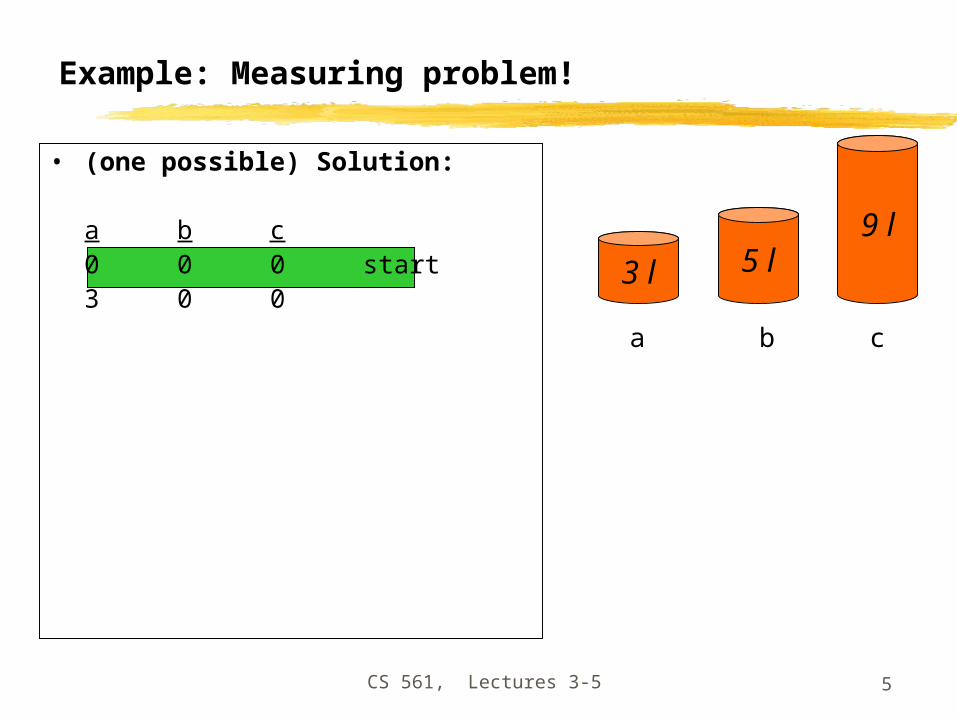
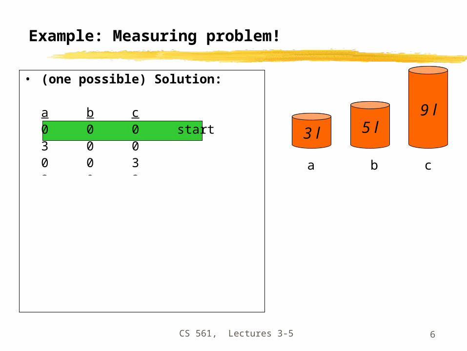
Example: Measuring problem!
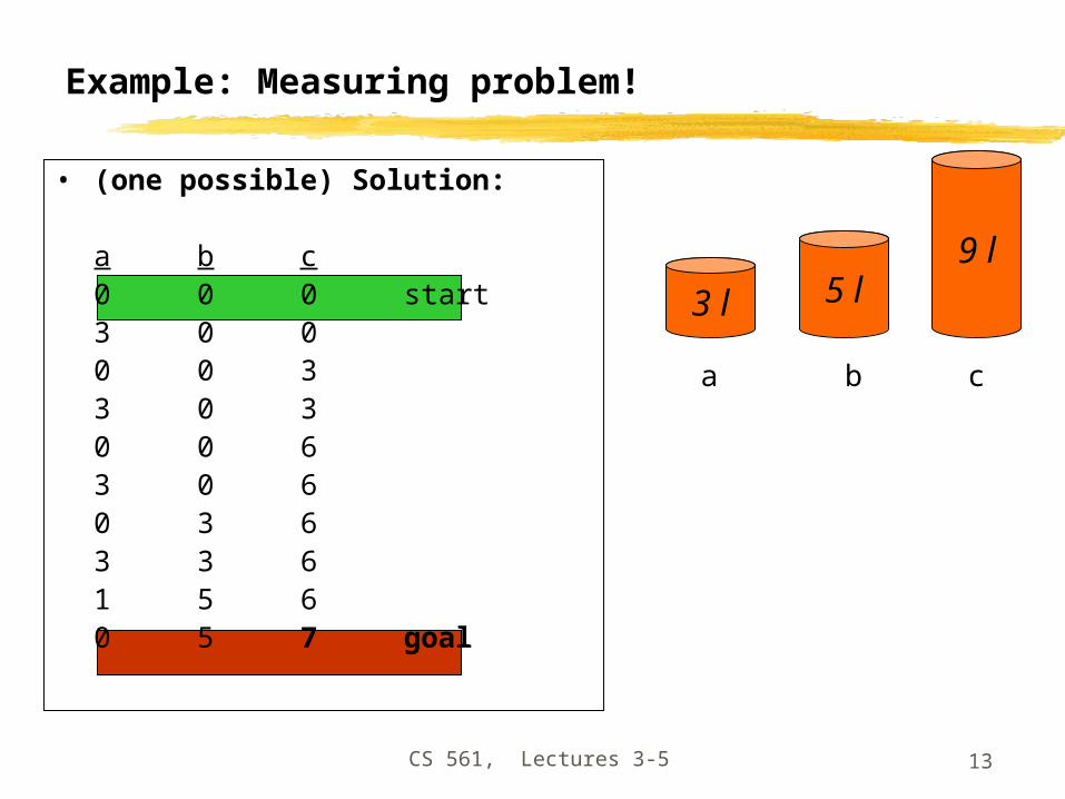
Problem: Using these three buckets,measure 7 liters of water.
3 l 5 l9 l

CS 561, Lectures 3-5 4
Example: Measuring problem!
• (one possible) Solution:
a b c0 0 0 start3 0 00 0 33 0 30 0 63 0 60 3 63 3 61 5 60 5 7 goal
3 l 5 l9 l
a b c
CS 561, Lectures 3-5 5
Example: Measuring problem!
• (one possible) Solution:
a b c0 0 0 start3 0 00 0 33 0 30 0 63 0 60 3 63 3 61 5 60 5 7 goal
3 l 5 l9 l
a b c
CS 561, Lectures 3-5 6
Example: Measuring problem!
• (one possible) Solution:
a b c0 0 0 start3 0 00 0 33 0 30 0 63 0 60 3 63 3 61 5 60 5 7 goal
3 l 5 l9 l
a b c

CS 561, Lectures 3-5 7
Example: Measuring problem!
• (one possible) Solution:
a b c0 0 0 start3 0 00 0 33 0 30 0 63 0 60 3 63 3 61 5 60 5 7 goal
3 l 5 l9 l
a b c

CS 561, Lectures 3-5 8
Example: Measuring problem!
• (one possible) Solution:
a b c0 0 0 start3 0 00 0 33 0 30 0 63 0 60 3 63 3 61 5 60 5 7 goal
3 l 5 l9 l
a b c

CS 561, Lectures 3-5 9
Example: Measuring problem!
• (one possible) Solution:
a b c0 0 0 start3 0 00 0 33 0 30 0 63 0 60 3 63 3 61 5 60 5 7 goal
3 l 5 l9 l
a b c

CS 561, Lectures 3-5 10
Example: Measuring problem!
• (one possible) Solution:
a b c0 0 0 start3 0 00 0 33 0 30 0 63 0 60 3 63 3 61 5 60 5 7 goal
3 l 5 l9 l
a b c

CS 561, Lectures 3-5 11
Example: Measuring problem!
• (one possible) Solution:
a b c0 0 0 start3 0 00 0 33 0 30 0 63 0 60 3 63 3 61 5 60 5 7 goal
3 l 5 l9 l
a b c

CS 561, Lectures 3-5 12
Example: Measuring problem!
• (one possible) Solution:
a b c0 0 0 start3 0 00 0 33 0 30 0 63 0 60 3 63 3 61 5 60 5 7 goal
3 l 5 l9 l
a b c
CS 561, Lectures 3-5 13
Example: Measuring problem!
• (one possible) Solution:
a b c0 0 0 start3 0 00 0 33 0 30 0 63 0 60 3 63 3 61 5 60 5 7 goal
3 l 5 l9 l
a b c

CS 561, Lectures 3-5 14
Example: Measuring problem!
• Another Solution:
a b c0 0 0 start0 5 00 0 33 0 30 0 63 0 60 3 63 3 61 5 60 5 7 goal
3 l 5 l9 l
a b c

CS 561, Lectures 3-5 15
Example: Measuring problem!
• Another Solution:
a b c0 0 0 start0 5 03 2 00 0 33 0 30 0 63 0 60 3 63 3 61 5 60 5 7 goal
3 l 5 l9 l
a b c
CS 561, Lectures 3-5 16
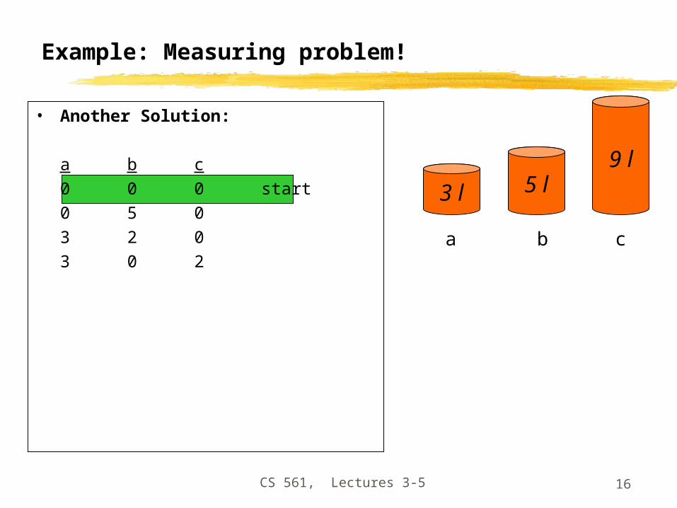
Example: Measuring problem!
• Another Solution:
a b c0 0 0 start0 5 03 2 03 0 23 0 30 0 63 0 60 3 63 3 61 5 60 5 7 goal
3 l 5 l9 l
a b c

CS 561, Lectures 3-5 17
Example: Measuring problem!
• Another Solution:
a b c0 0 0 start0 5 03 2 03 0 23 5 20 0 63 0 60 3 63 3 61 5 60 5 7 goal
3 l 5 l9 l
a b c

CS 561, Lectures 3-5 18
Example: Measuring problem!
• Another Solution:
a b c0 0 0 start0 5 03 2 03 0 23 5 23 0 7 goal3 0 60 3 63 3 61 5 60 5 7 goal
3 l 5 l9 l
a b c
CS 561, Lectures 3-5 19
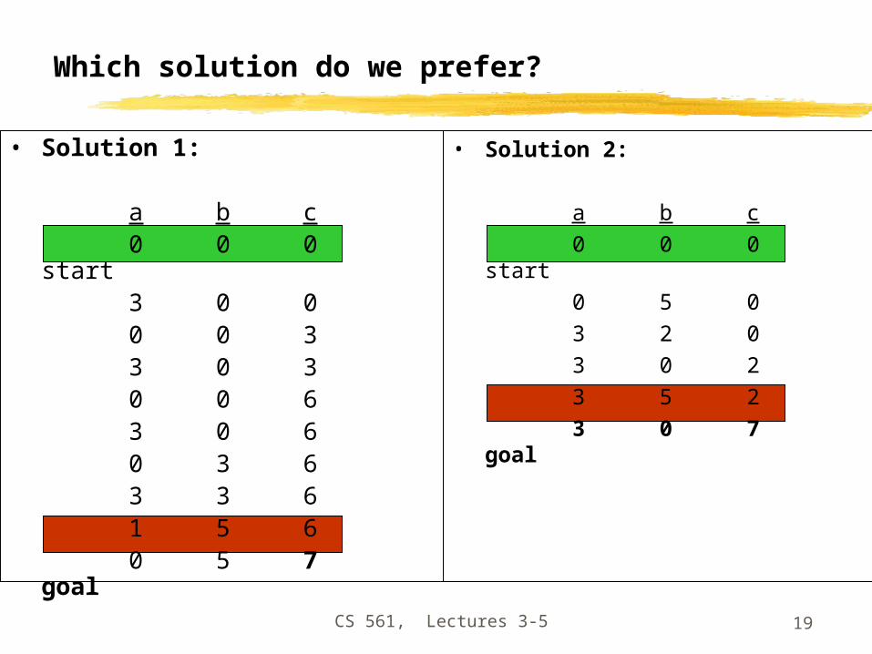
Which solution do we prefer?
• Solution 1:
a b c0 0 0
start3 0 00 0 33 0 30 0 63 0 60 3 63 3 61 5 60 5 7
goal
• Solution 2:
a b c0 0 0
start0 5 03 2 03 0 23 5 23 0 7
goal

CS 561, Lectures 3-5 20
Problem-Solving Agent
Note: This is offline problem-solving. Online problem-solving involves acting w/o complete knowledge of the problem and environment
action
// From LA to San Diego (given curr. state)
// e.g., Gas usage
// What is the current state?
// If fails to reach goal, update

CS 561, Lectures 3-5 21
Example: Buckets
Measure 7 liters of water using a 3-liter, a 5-liter, and a 9-liter buckets.
• Formulate goal:Have 7 liters of waterin 9-liter bucket
• Formulate problem:• States: amount of water in the buckets• Operators: Fill bucket from source, empty bucket
• Find solution: sequence of operators that bring youfrom current state to the goal state

CS 561, Lectures 3-5 22
Remember (lecture 2): Environment types
Environment Accessible
Deterministic
Episodic Static Discrete
Operating System
Yes Yes No No Yes
Virtual Reality
Yes Yes Yes/No No Yes/No
Office Environment
No No No No No
Mars No Semi No Semi No
The environment types largely determine the agent design.

CS 561, Lectures 3-5 23
Problem types
• Single-state problem: deterministic, accessibleAgent knows everything about world, thus can
calculate optimal action sequence to reach goal state.
• Multiple-state problem: deterministic, inaccessibleAgent must reason about sequences of actions and
states assumed while working towards goal state.
• Contingency problem: nondeterministic, inaccessible• Must use sensors during execution• Solution is a tree or policy• Often interleave search and execution
• Exploration problem: unknown state spaceDiscover and learn about environment while taking actions.

CS 561, Lectures 3-5 24
Problem types
• Single-state problem: deterministic, accessible
• Agent knows everything about world (the exact state),
• Can calculate optimal action sequence to reach goal state.
• E.g., playing chess. Any action will result in an exact state

CS 561, Lectures 3-5 25
Problem types
• Multiple-state problem: deterministic, inaccessible
• Agent does not know the exact state (could be in any of the possible states)
• May not have sensor at all
• Assume states while working towards goal state.
• E.g., walking in a dark room• If you are at the door, going straight will lead you to the kitchen• If you are at the kitchen, turning left leads you to the bedroom• …

CS 561, Lectures 3-5 26
Problem types
• Contingency problem: nondeterministic, inaccessible
• Must use sensors during execution• Solution is a tree or policy• Often interleave search and execution
• E.g., a new skater in an arena• Sliding problem.• Many skaters around

CS 561, Lectures 3-5 27
Problem types
• Exploration problem:unknown state space
Discover and learn about environment while taking actions.
• E.g., Maze

CS 561, Lectures 3-5 28
Example: Vacuum world
Simplified world: 2 locations, each may or not contain dirt,each may or not contain vacuuming agent.
Goal of agent: clean up the dirt.

CS 561, Lectures 3-5 29

CS 561, Lectures 3-5 30

CS 561, Lectures 3-5 31

CS 561, Lectures 3-5 32
Example: Romania
• In Romania, on vacation. Currently in Arad.• Flight leaves tomorrow from Bucharest.
• Formulate goal:be in Bucharest
• Formulate problem:states: various citiesoperators: drive between cities
• Find solution:sequence of cities, such that total driving
distance is minimized.

CS 561, Lectures 3-5 33
Example: Traveling from Arad To Bucharest

CS 561, Lectures 3-5 34
Problem formulation

CS 561, Lectures 3-5 35
Selecting a state space
• Real world is absurdly complex; some abstraction is necessary to allow us to reason on it…
• Selecting the correct abstraction and resulting state space is a difficult problem!
• Abstract states real-world states
• Abstract operators sequences or real-world actions(e.g., going from city i to city j costs Lij actually drive from city i to j)
• Abstract solution set of real actions to take in thereal world such as to solve problem

CS 561, Lectures 3-5 36
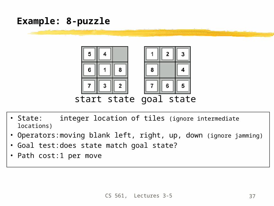
Example: 8-puzzle
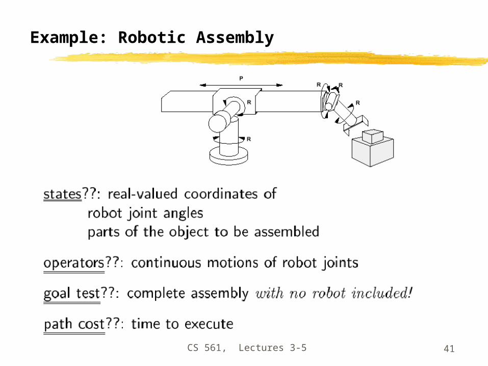
• State: • Operators:• Goal test:• Path cost:
start state goal state
CS 561, Lectures 3-5 37
• State: integer location of tiles (ignore intermediate locations)
• Operators: moving blank left, right, up, down (ignore jamming)
• Goal test: does state match goal state?• Path cost: 1 per move
Example: 8-puzzle
start state goal state

CS 561, Lectures 3-5 38
Example: 8-puzzle
start state goal state
Why search algorithms?• 8-puzzle has 362,800 states• 15-puzzle has 10^12 states• 24-puzzle has 10^25 states
So, we need a principled way to look for a solution in these huge search spaces…

CS 561, Lectures 3-5 39
Back to Vacuum World

CS 561, Lectures 3-5 40
Back to Vacuum World
CS 561, Lectures 3-5 41
Example: Robotic Assembly

CS 561, Lectures 3-5 42
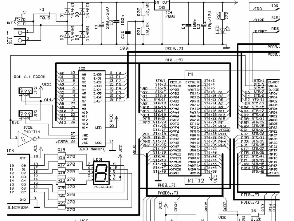
Real-life example: VLSI Layout
• Given schematic diagram comprising components (chips, resistors, capacitors, etc) and interconnections (wires), find optimal way to place components on a printed circuit board, under the constraint that only a small number of wire layers are available (and wires on a given layer cannot cross!)
• “optimal way”??
minimize surface area minimize number of signal layers minimize number of vias (connections from one layer to
another) minimize length of some signal lines (e.g., clock line) distribute heat throughout board etc.

CS 561, Lectures 3-5 43
En
ter
sch
em
ati
cs;
do n
ot
worr
y a
bout
pla
cem
en
t &
wir
e c
ross
ing
CS 561, Lectures 3-5 44

CS 561, Lectures 3-5 45
Use
auto
mate
d t
ools
to p
lace
com
pon
en
tsand
route
wir
ing
.

CS 561, Lectures 3-5 46

CS 561, Lectures 3-5 47
Function General-Search(problem, strategy) returns a solution, or failureinitialize the search tree using the initial state problemloop do
if there are no candidates for expansion then return failurechoose a leaf node for expansion according to strategyif the node contains a goal state then
return the corresponding solutionelse expand the node and add resulting nodes to the search
treeend
Search algorithms
Basic idea:
offline, systematic exploration of simulated state-space by generating successors of explored states (expanding)

CS 561, Lectures 3-5 48
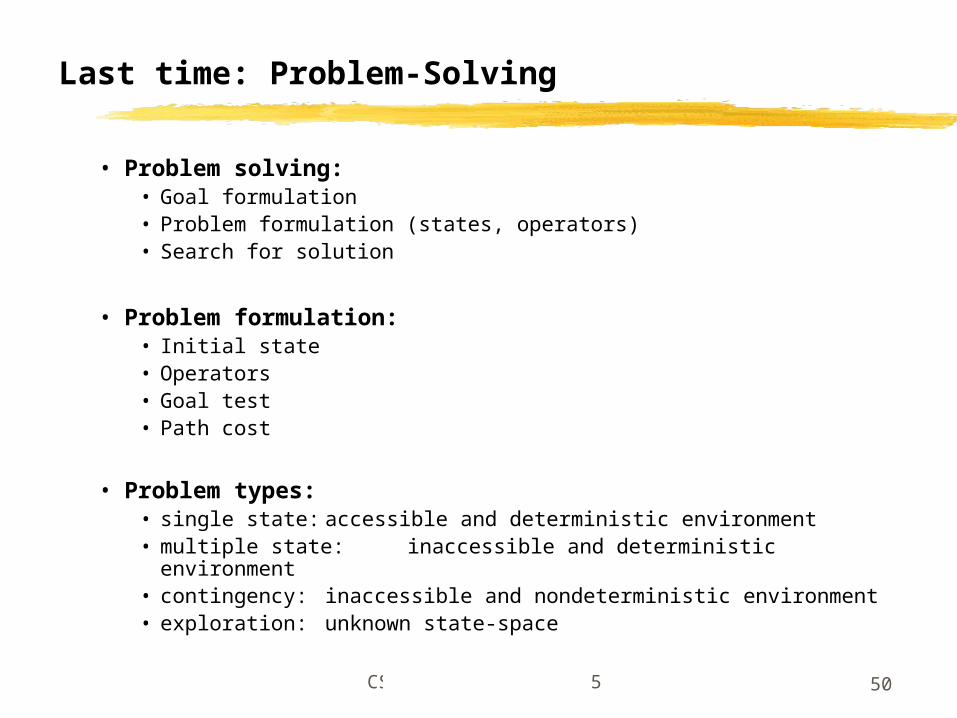
Last time: Problem-Solving
• Problem solving: • Goal formulation • Problem formulation (states, operators) • Search for solution
• Problem formulation:• Initial state• ?• ?• ?
• Problem types: • single state: accessible and deterministic environment• multiple state: ?• contingency: ?• exploration: ?

CS 561, Lectures 3-5 49
Last time: Problem-Solving
• Problem solving: • Goal formulation • Problem formulation (states, operators) • Search for solution
• Problem formulation:• Initial state• Operators• Goal test• Path cost
• Problem types: • single state: accessible and deterministic environment• multiple state: ?• contingency: ?• exploration: ?
CS 561, Lectures 3-5 50
Last time: Problem-Solving
• Problem solving: • Goal formulation • Problem formulation (states, operators) • Search for solution
• Problem formulation:• Initial state• Operators• Goal test• Path cost
• Problem types: • single state: accessible and deterministic environment• multiple state: inaccessible and deterministic environment• contingency: inaccessible and nondeterministic environment• exploration: unknown state-space

CS 561, Lectures 3-5 51
Last time: Finding a solution
Function General-Search(problem, strategy) returns a solution, or failureinitialize the search tree using the initial state problemloop do
if there are no candidates for expansion then return failurechoose a leaf node for expansion according to strategyif the node contains a goal state then return the corresponding
solutionelse expand the node and add resulting nodes to the search tree
end
Solution: is ???
Basic idea: offline, systematic exploration of simulated state-space by generating successors of explored states (expanding)

CS 561, Lectures 3-5 52
Last time: Finding a solution
Function General-Search(problem, strategy) returns a solution, or failureinitialize the search tree using the initial state problemloop do
if there are no candidates for expansion then return failurechoose a leaf node for expansion according to strategyif the node contains a goal state then return the corresponding
solutionelse expand the node and add resulting nodes to the search tree
end
Solution: is a sequence of operators that bring you from current state to the goal state.
Basic idea: offline, systematic exploration of simulated state-space by generating successors of explored states (expanding).
Strategy: The search strategy is determined by ???

CS 561, Lectures 3-5 53
Last time: Finding a solution
Function General-Search(problem, strategy) returns a solution, or failureinitialize the search tree using the initial state problemloop do
if there are no candidates for expansion then return failurechoose a leaf node for expansion according to strategyif the node contains a goal state then return the corresponding
solutionelse expand the node and add resulting nodes to the search tree
end
Solution: is a sequence of operators that bring you from current state to the goal state
Basic idea: offline, systematic exploration of simulated state-space by generating successors of explored states (expanding)
Strategy: The search strategy is determined by the order in which the nodes are expanded.

CS 561, Lectures 3-5 54
Example: Traveling from Arad To Bucharest

CS 561, Lectures 3-5 55
From problem space to search tree
• Some material in this and following slides is fromhttp://www.cs.kuleuven.ac.be/~dannyd/FAI/ check it
out!
AA
DD
BB
EE
CC
FFGG
SS33
44
44
44
55 55
44
3322
SSAA DD
BB DD EEAA
CC EE EE BB BB FF
DD FF BB FF CC EE AA CC GG
GG CC GG FF
GG
33
33 33
33
33
22
22
2244
44
4444
44
4444
44
44
44
44
44
5555
55 55
5555
Problem space
Associatedloop-freesearch tree

CS 561, Lectures 3-5 56
Paths in search trees
SSAA DD
BB DD EEAA
CC EE EE BB BB FF
DD FF BB FF CC EE AA CC GG
GG CC GG FF
GG
Denotes:Denotes:SASA Denotes:Denotes:SDSD
AA
DenotesDenotes:: SDEBASDEBA

CS 561, Lectures 3-5 57
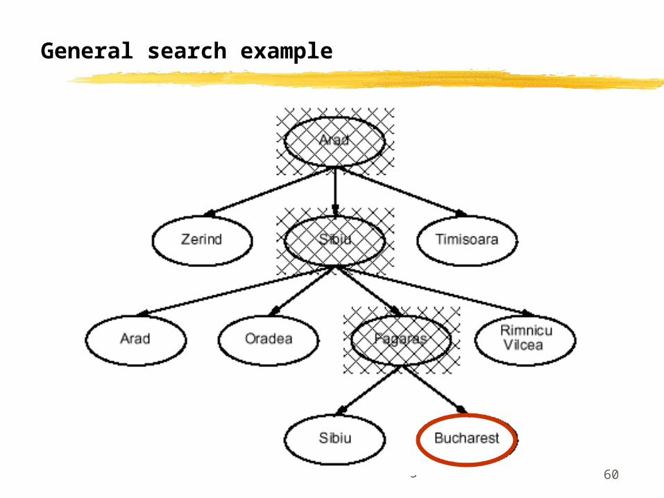
General search example

CS 561, Lectures 3-5 58
General search example

CS 561, Lectures 3-5 59
General search example
CS 561, Lectures 3-5 60
General search example

CS 561, Lectures 3-5 61
Implementation of search algorithms
Function General-Search(problem, Queuing-Fn) returns a solution, or failurenodes make-queue(make-node(initial-state[problem]))loop doif nodes is empty then return failurenode Remove-Front(nodes)if Goal-Test[problem] applied to State(node) succeeds then return nodenodes Queuing-Fn(nodes, Expand(node, Operators[problem]))end
Queuing-Fn(queue, elements) is a queuing function that inserts a set of elements into the queue and determines the order of node expansion. Varieties of the queuing function produce varieties of the search algorithm.

CS 561, Lectures 3-5 62
Encapsulating state information in nodes

CS 561, Lectures 3-5 63
Evaluation of search strategies
• A search strategy is defined by picking the order of node expansion.
• Search algorithms are commonly evaluated according to the following four criteria:• Completeness: does it always find a solution if one exists?• Time complexity: how long does it take as function of num. of
nodes?• Space complexity: how much memory does it require?• Optimality: does it guarantee the least-cost solution?
• Time and space complexity are measured in terms of:• b – max branching factor of the search tree• d – depth of the least-cost solution• m – max depth of the search tree (may be infinity)

CS 561, Lectures 3-5 64
Binary Tree Example
root
N1 N2
N3 N4 N5 N6
Number of nodes: n = 2 max depth
Number of levels (max depth) = log(n) (could be n)
Depth = 0
Depth = 1
Depth = 2

CS 561, Lectures 3-5 65
Complexity
• Why worry about complexity of algorithms?
because a problem may be solvable in principle but may take too long to solve in practice
CS 561, Lectures 3-5 66
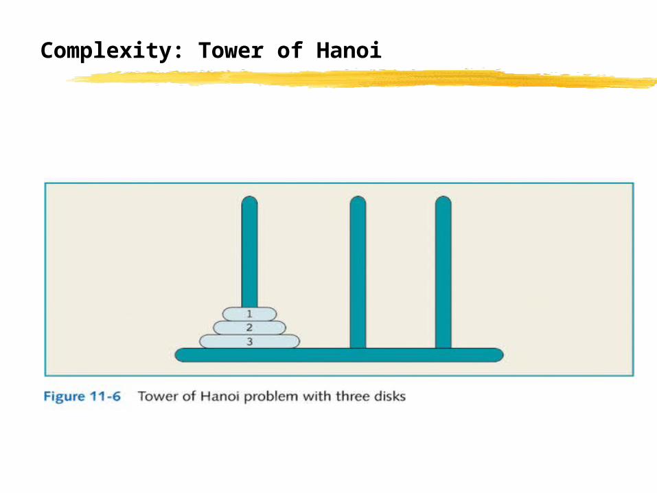
Complexity: Tower of Hanoi

CS 561, Lectures 3-5 67
Complexity:Tower of Hanoi

CS 561, Lectures 3-5 68
Complexity: Tower of Hanoi
3-disk problem: 23 - 1 = 7 moves
64-disk problem: 264 - 1. 210 = 1024 1000 = 103, 264 = 24 * 260 24 * 1018 = 1.6 * 1019
One year 3.2 * 107 seconds

CS 561, Lectures 3-5 69
Complexity: Tower of Hanoi
The wizard’s speed = one disk / second
1.6 * 1019 = 5 * 3.2 * 1018 =
5 * (3.2 * 107) * 1011 =
(3.2 * 107) * (5 * 1011)
CS 561, Lectures 3-5 70
Complexity: Tower of Hanoi
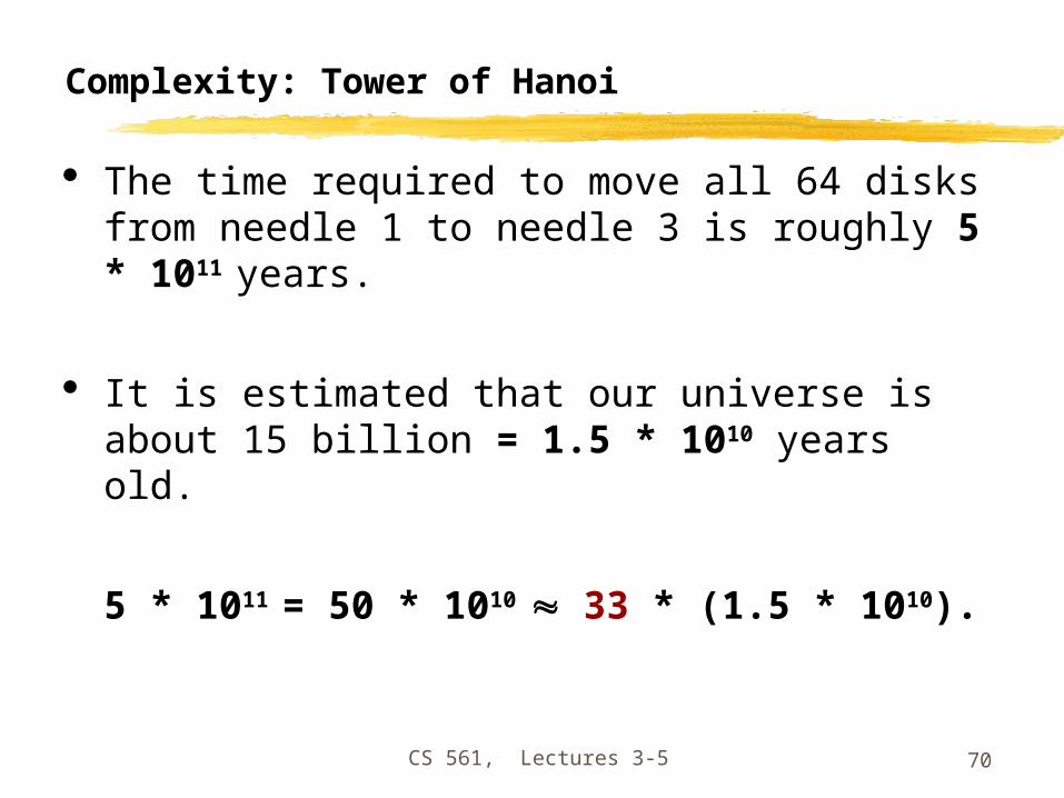
The time required to move all 64 disks from needle 1 to needle 3 is roughly 5 * 1011
years.
It is estimated that our universe is about 15 billion = 1.5 * 1010 years old.
5 * 1011 = 50 * 1010 33 * (1.5 * 1010).

CS 561, Lectures 3-5 71
Complexity: Tower of Hanoi
Assume: a computer with 1 billion = 109 moves/second. Moves/year=(3.2 *107) * 109 = 3.2 * 1016
To solve the problem for 64 disks: 264 1.6 * 1019 = 1.6 * 1016 * 103 =
(3.2 * 1016) * 500
500 years for the computer to generate 264 moves at the rate of 1 billion moves per second.

CS 561, Lectures 3-5 72
Complexity
• Why worry about complexity of algorithms? because a problem may be solvable in principle
but may take too long to solve in practice
• How can we evaluate the complexity of algorithms?
through asymptotic analysis, i.e., estimate time (or number of operations) necessary to solve an instance of size n of a problem when n tends towards infinity
See AIMA, Appendix A.

CS 561, Lectures 3-5 73
Complexity example: Traveling Salesman Problem
• There are n cities, with a road of length Lij joining city i to city j.
• The salesman wishes to find a way to visit all cities that
is optimal in two ways:each city is visited only once, and the total route is as short as possible.

CS 561, Lectures 3-5 74
Complexity example: Traveling Salesman Problem
This is a hard problem: the only known algorithms (so far) to solve it have exponential complexity, that is, the number of operations required to solve it grows as exp(n) for n cities.

CS 561, Lectures 3-5 75
Why is exponential complexity “hard”?
It means that the number of operations necessary to compute the exact solution of the problem grows exponentially with the size of the problem (here, the number of cities).
• exp(1) = 2.72• exp(10) = 2.20 104 (daily salesman trip)• exp(100) = 2.69 1043 (monthly salesman planning)• exp(500) = 1.40 10217 (music band worldwide tour)• exp(250,000) = 10108,573 (fedex, postal services)• Fastest
computer = 1012 operations/second
CS 561, Lectures 3-5 76
So…
In general, exponential-complexity problems cannot be solved for any but the smallest instances!

CS 561, Lectures 3-5 77
Complexity
• Polynomial-time (P) problems: we can find algorithms that will solve them in a time (=number of operations) that grows polynomially with the size of the input.
for example: sort n numbers into increasing order: poor algorithms have n^2 complexity, better ones have n log(n) complexity.

CS 561, Lectures 3-5 78
Complexity
• Since we did not state what the order of the polynomial is, it could be very large! Are there algorithms that require more than polynomial time?
• Yes (until proof of the contrary); for some algorithms, we do not know of any polynomial-time algorithm to solve them. These belong to the class of nondeterministic-polynomial-time (NP) algorithms (which includes P problems as well as harder ones).
for example: traveling salesman problem.
• In particular, exponential-time algorithms are believed to be NP.

CS 561, Lectures 3-5 79
Note on NP-hard problems
• The formal definition of NP problems is:
A problem is nondeterministic polynomial if there exists some algorithm that can guess a solution and then verify whether or not the guess is correct in polynomial time.
(one can also state this as these problems being solvable in polynomial time on a nondeterministic Turing machine.)
In practice, until proof of the contrary, this means that known algorithms that run on known computer architectures will take more than polynomial time to solve the problem.

CS 561, Lectures 3-5 80
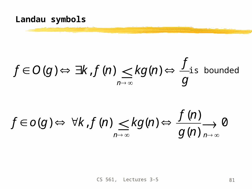
Complexity: O() and o() measures (Landau symbols)
• How can we represent the complexity of an algorithm?
• Given: Problem input (or instance) size: nNumber of operations to solve problem: f(n)
• If, for a given function g(n), we have:
then f is dominated by g
• If, for a given function g(n), we have:
then f is negligible compared to g
)(
)()(,,,, 00
gOf
nkgnfnnnnk
)(
)()(,,,, 00
gof
nkgnfnnnnk
CS 561, Lectures 3-5 81
Landau symbols
0)(
)()()(,)(
nn ng
nfnkgnfkgof
g
fnkgnfkgOf
n
)()(,)( is bounded

CS 561, Lectures 3-5 82
Examples, properties
• f(n)=n, g(n)=n^2:n is o(n^2), because n/n^2 = 1/n -> 0 as n -
>infinitysimilarly, log(n) is o(n)
n^C is o(exp(n)) for any C
• if f is O(g), then for any K, K.f is also O(g); idem for o()• if f is O(h) and g is O(h), then for any K, L: K.f + L.g is O(h)
idem for o()
• if f is O(g) and g is O(h), then f is O(h)• if f is O(g) and g is o(h), then f is o(h)• if f is o(g) and g is O(h), then f is o(h)

CS 561, Lectures 3-5 83
Polynomial-time hierarchy
• From Handbook of BrainTheory & Neural Networks(Arbib, ed.;MIT Press 1995).
AC0 NC1 NC P complete NP complete
PNP
PH
AC0: can be solved using gates of constant depthNC1: can be solved in logarithmic depth using 2-input gatesNC: can be solved by small, fast parallel computerP: can be solved in polynomial timeP-complete: hardest problems in P; if one of them can be proven to be
NC, then P = NCNP: nondeterministic-polynomial algorithmsNP-complete: hardest NP problems; if one of them can be proven to be
P, then NP = PPH: polynomial-time hierarchy

CS 561, Lectures 3-5 84
Complexity and the human brain
• Are computers close to human brain power?
• Current computer chip (CPU):• 10^3 inputs (pins)• 10^7 processing elements (gates)• 2 inputs per processing element (fan-in = 2)• processing elements compute boolean logic (OR, AND,
NOT, etc)
• Typical human brain:• 10^7 inputs (sensors)• 10^10 processing elements (neurons)• fan-in = 10^3• processing elements compute complicated
functionsStill a lot of improvement needed for computers; butcomputer clusters come close!

CS 561, Lectures 3-5 85
Remember: Implementation of search algorithms
Function General-Search(problem, Queuing-Fn) returns a solution, or failurenodes make-queue(make-node(initial-state[problem]))loop doif nodes is empty then return failurenode Remove-Front(nodes)if Goal-Test[problem] applied to State(node) succeeds then return nodenodes Queuing-Fn(nodes, Expand(node, Operators[problem]))end
Queuing-Fn(queue, elements) is a queuing function that inserts a set of elements into the queue and determines the order of node expansion. Varieties of the queuing function produce varieties of the search algorithm.

CS 561, Lectures 3-5 86
Encapsulating state information in nodes

CS 561, Lectures 3-5 87
Evaluation of search strategies
• A search strategy is defined by picking the order of node expansion.
• Search algorithms are commonly evaluated according to the following four criteria:• Completeness: does it always find a solution if one exists?• Time complexity: how long does it take as function of num. of
nodes?• Space complexity: how much memory does it require?• Optimality: does it guarantee the least-cost solution?
• Time and space complexity are measured in terms of:• b – max branching factor of the search tree• d – depth of the least-cost solution• m – max depth of the search tree (may be infinity)

CS 561, Lectures 3-5 88
Note: Approximations
• In our complexity analysis, we do not take the built-in loop-detection into account.
• The results only ‘formally’ apply to the variants of our algorithms WITHOUT loop-checks.
• Studying the effect of the loop-checking on the complexity is hard: • overhead of the checking MAY or MAY NOT be compensated
by the reduction of the size of the tree.
• Also: our analysis DOES NOT take the length (space) of representing paths into account !!
http://www.cs.kuleuven.ac.be/~dannyd/FAI/

CS 561, Lectures 3-5 89
Uninformed search strategies
Use only information available in the problem formulation
• Breadth-first• Uniform-cost• Depth-first• Depth-limited• Iterative deepening

CS 561, Lectures 3-5 90
Breadth-first search

CS 561, Lectures 3-5 91
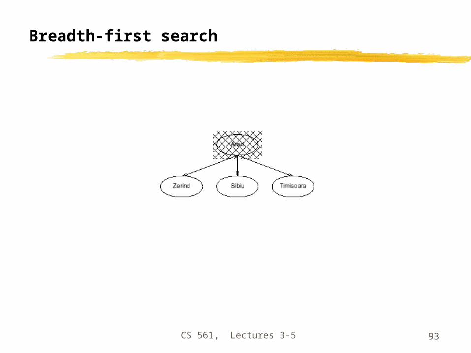
Breadth-first search
Move downwards, level by level, until goal is reached.
SS
AA DD
BB DD AA EE
CC EE EE BB BB FF
DD FF BB FF CC EE AA CC GG
GG
GGGG FFCC

CS 561, Lectures 3-5 92
Example: Traveling from Arad To Bucharest
CS 561, Lectures 3-5 93
Breadth-first search

CS 561, Lectures 3-5 94
Breadth-first search

CS 561, Lectures 3-5 95
Breadth-first search

CS 561, Lectures 3-5 96
Properties of breadth-first search
• Completeness:• Time complexity:• Space complexity:• Optimality:
• Search algorithms are commonly evaluated according to the following four criteria:
• Completeness: does it always find a solution if one exists?• Time complexity: how long does it take as function of num. of nodes?• Space complexity: how much memory does it require?• Optimality: does it guarantee the least-cost solution?
• Time and space complexity are measured in terms of:• b – max branching factor of the search tree• d – depth of the least-cost solution• m – max depth of the search tree (may be infinity)
CS 561, Lectures 3-5 97
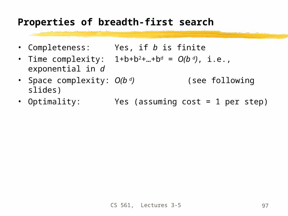
Properties of breadth-first search
• Completeness: Yes, if b is finite• Time complexity: 1+b+b2+…+bd = O(b d), i.e.,
exponential in d• Space complexity: O(b d) (see following slides)• Optimality: Yes (assuming cost = 1 per step)

CS 561, Lectures 3-5 98
Time complexity of breadth-first search
• If a goal node is found on depth d of the tree, all nodes up till that depth are created.
mmGGbb
dd
• Thus: O(bd)

CS 561, Lectures 3-5 99
• QUEUE contains all and nodes. (Thus: 4) .
• In General: bd
Space complexity of breadth-first
• Largest number of nodes in QUEUE is reached on the level d of the goal node.
GGmmbb
dd
GG

CS 561, Lectures 3-5 100
Uniform-cost search
So, the queueing function keeps the node list sorted by increasing path cost, and we expand the first unexpanded node (hence with smallest path cost)
A refinement of the breadth-first strategy:
Breadth-first = uniform-cost with path cost = node depth

CS 561, Lectures 3-5 101
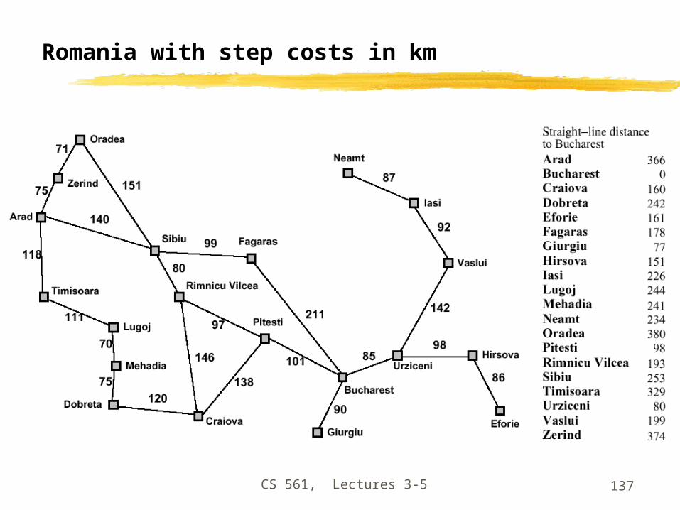
Romania with step costs in km

CS 561, Lectures 3-5 102
Uniform-cost search

CS 561, Lectures 3-5 103
Uniform-cost search

CS 561, Lectures 3-5 104
Uniform-cost search

CS 561, Lectures 3-5 105
Properties of uniform-cost search
• Completeness: Yes, if step cost >0• Time complexity: # nodes with g cost of optimal solution,
O(b d)
• Space complexity: # nodes with g cost of optimal solution, O(b d)
• Optimality: Yes, as long as path cost never decreases
g(n) is the path cost to node nRemember:
b = branching factord = depth of least-cost solution

CS 561, Lectures 3-5 106
Implementation of uniform-cost search
• Initialize Queue with root node (built from start state)
• Repeat until (Queue empty) or (first node has Goal state):
• Remove first node from front of Queue• Expand node (find its children)• Reject those children that have already been considered, to
avoid loops• Add remaining children to Queue, in a way that keeps
entire queue sorted by increasing path cost
• If Goal was reached, return success, otherwise failure
CS 561, Lectures 3-5 107
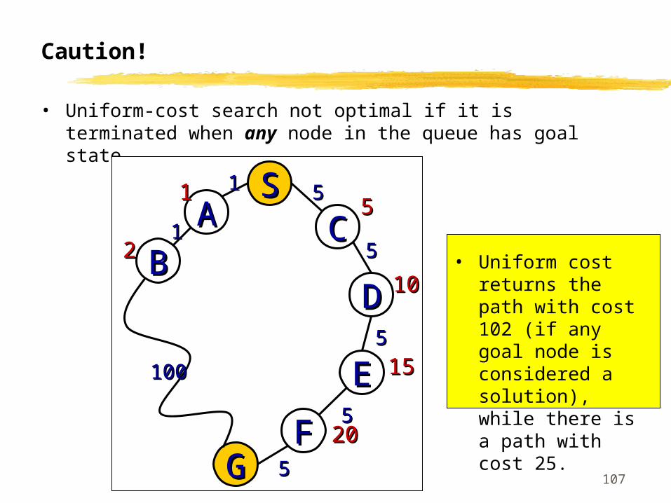
Caution!
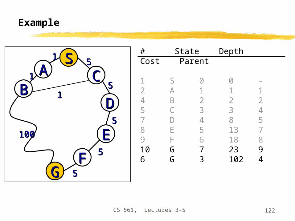
• Uniform-cost search not optimal if it is terminated when any node in the queue has goal state.
GG
100100
55
DD
55
1010
EE55
1515
FF55
2020
SSAA CC
11 5555
11
BB11
22 • Uniform cost returns the path with cost 102 (if any goal node is considered a solution), while there is a path with cost 25.
CS 561, Lectures 3-5 108
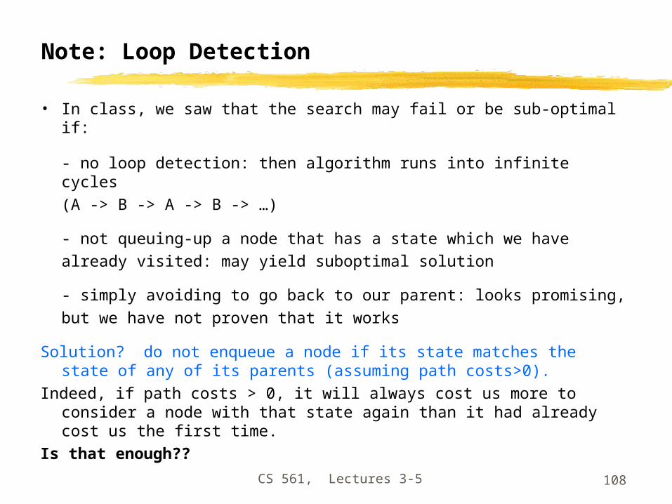
Note: Loop Detection
• In class, we saw that the search may fail or be sub-optimal if:
- no loop detection: then algorithm runs into infinite cycles(A -> B -> A -> B -> …)
- not queuing-up a node that has a state which we havealready visited: may yield suboptimal solution
- simply avoiding to go back to our parent: looks promising, but we have not proven that it works
Solution? do not enqueue a node if its state matches the state of any of its parents (assuming path costs>0).
Indeed, if path costs > 0, it will always cost us more to consider a node with that state again than it had already cost us the first time.
Is that enough??

CS 561, Lectures 3-5 109
Example
G
From: http://www.csee.umbc.edu/471/current/notes/uninformed-search/
CS 561, Lectures 3-5 110
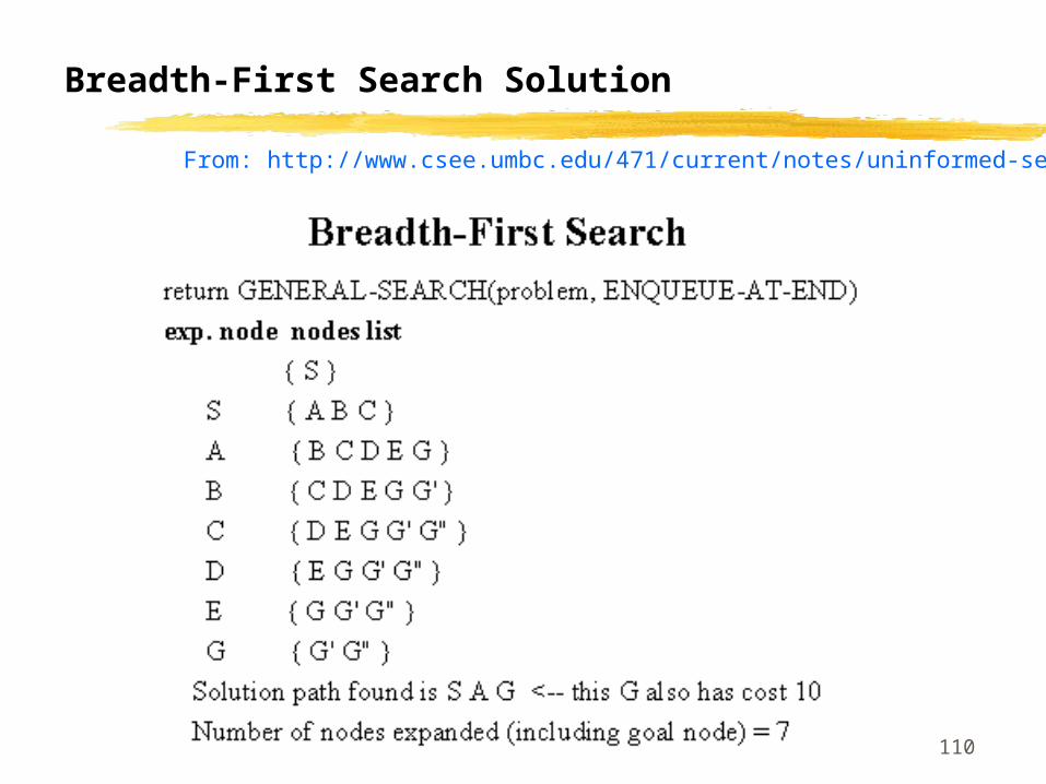
Breadth-First Search Solution
From: http://www.csee.umbc.edu/471/current/notes/uninformed-search/

CS 561, Lectures 3-5 111
Uniform-Cost Search Solution
From: http://www.csee.umbc.edu/471/current/notes/uninformed-search/

CS 561, Lectures 3-5 112
Note: Queueing in Uniform-Cost Search
In the previous example, it is wasteful (but not incorrect) to queue-up three nodes with G state, if our goal if to find the least-cost solution:
Although they represent different paths, we know for sure that the one with smallest path cost (9 in the example) will yield a solution with smaller total path cost than the others.
So we can refine the queueing function by:- queue-up node if
1) its state does not match the state of any parentand 2) path cost smaller than path cost of any
unexpanded node with same state in the queue (and in this case, replace old node with same
state by our new node)Is that it??

CS 561, Lectures 3-5 113
A Clean Robust Algorithm
Function UniformCost-Search(problem, Queuing-Fn) returns a solution, or failureopen make-queue(make-node(initial-state[problem]))closed [empty]loop do
if open is empty then return failurecurrnode Remove-Front(open)if Goal-Test[problem] applied to State(currnode) then return
currnodechildren Expand(currnode, Operators[problem])while children not empty
[… see next slide …]endclosed Insert(closed, currnode)open Sort-By-PathCost(open)
end

CS 561, Lectures 3-5 114
A Clean Robust Algorithm
[… see previous slide …]children Expand(currnode, Operators[problem])while children not empty
child Remove-Front(children)if no node in open or closed has child’s state
open Queuing-Fn(open, child)else if there exists node in open that has child’s state
if PathCost(child) < PathCost(node)open Delete-Node(open, node)open Queuing-Fn(open, child)
else if there exists node in closed that has child’s state
if PathCost(child) < PathCost(node)closed Delete-Node(closed, node)open Queuing-Fn(open, child)
end[… see previous slide …]

CS 561, Lectures 3-5 115
Example
GG
100100
55
DD55
EE55
FF 55
SSAA CC
1155
BB11
11
# State Depth Cost Parent
1 S 0 0 -

CS 561, Lectures 3-5 116
Example
GG
100100
55
DD55
EE55
FF 55
SSAA CC
1155
BB11
11
# State Depth Cost Parent
1 S 0 0 -2 A 1 1 13 C 1 5 1
Insert expanded nodesSuch as to keep open queuesorted
Black = open queueGrey = closed queue

CS 561, Lectures 3-5 117
Example
GG
100100
55
DD55
EE55
FF 55
SSAA CC
1155
BB11
11
# State Depth Cost Parent
1 S 0 0 -2 A 1 1 14 B 2 2 23 C 1 5 1
Node 2 has 2 successors: one with state Band one with state S.
We have node #1 in closed with state S;but its path cost 0 is smaller than the pathcost obtained by expanding from A to S.So we do not queue-up the successor ofnode 2 that has state S.

CS 561, Lectures 3-5 118
Example
GG
100100
55
DD55
EE55
FF 55
SSAA CC
1155
BB11
11
# State Depth Cost Parent
1 S 0 0 -2 A 1 1 14 B 2 2 25 C 3 3 46 G 3 102 4
Node 4 has a successor with state C andCost smaller than node #3 in open thatAlso had state C; so we update openTo reflect the shortest path.

CS 561, Lectures 3-5 119
Example
GG
100100
55
DD55
EE55
FF 55
SSAA CC
1155
BB11
11
# State Depth Cost Parent
1 S 0 0 -2 A 1 1 14 B 2 2 25 C 3 3 47 D 4 8 56 G 3 102 4

CS 561, Lectures 3-5 120
Example
GG
100100
55
DD55
EE55
FF 55
SSAA CC
1155
BB11
11
# State Depth Cost Parent
1 S 0 0 -2 A 1 1 14 B 2 2 25 C 3 3 47 D 4 8 58 E 5 13 76 G 3 102 4

CS 561, Lectures 3-5 121
Example
GG
100100
55
DD55
EE55
FF 55
SSAA CC
1155
BB11
11
# State Depth Cost Parent
1 S 0 0 -2 A 1 1 14 B 2 2 25 C 3 3 47 D 4 8 58 E 5 13 79 F 6 18 86 G 3 102 4
CS 561, Lectures 3-5 122
Example
GG
100100
55
DD55
EE55
FF 55
SSAA CC
1155
BB11
11
# State Depth Cost Parent
1 S 0 0 -2 A 1 1 14 B 2 2 25 C 3 3 47 D 4 8 58 E 5 13 79 F 6 18 810 G 7 23 96 G 3 102 4

CS 561, Lectures 3-5 123
Example
GG
100100
55
DD55
EE55
FF 55
SSAA CC
1155
BB11
11
# State Depth Cost Parent
1 S 0 0 -2 A 1 1 14 B 2 2 25 C 3 3 47 D 4 8 58 E 5 13 79 F 6 18 810 G 7 23 96 G 3 102 4
Goal reached

CS 561, Lectures 3-5 124
More examples…
• See the great demos at:
http://pages.pomona.edu/~jbm04747/courses/spring2001/cs151/Search/Strategies.html

CS 561, Lectures 3-5 125
Depth-first search
CS 561, Lectures 3-5 126
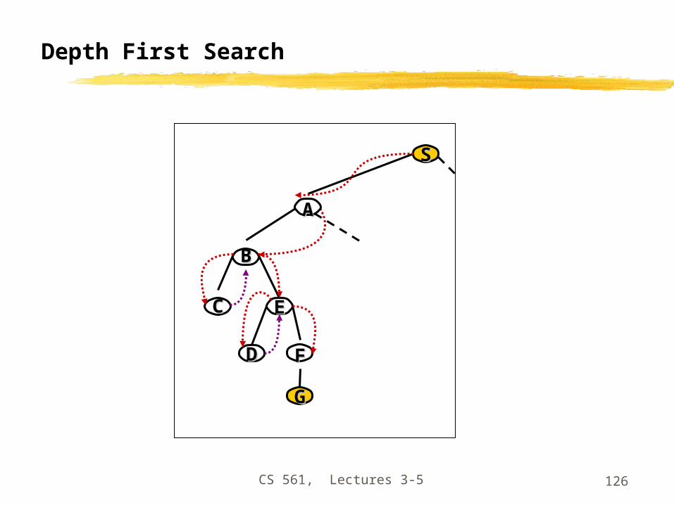
Depth First Search
BB
CC EE
DD FF
GG
SS
AA

CS 561, Lectures 3-5 127
Romania with step costs in km

CS 561, Lectures 3-5 128
Depth-first search

CS 561, Lectures 3-5 129
Depth-first search

CS 561, Lectures 3-5 130
Depth-first search

CS 561, Lectures 3-5 131
Properties of depth-first search
• Completeness: No, fails in infinite state-space (yes if finite state space)
• Time complexity: O(b m)• Space complexity: O(bm)• Optimality: No
Remember:
b = branching factor
m = max depth of search tree

CS 561, Lectures 3-5 132
Time complexity of depth-first: details
• In the worst case: • the (only) goal node may be on the right-most branch,
GG
mmbb
• Time complexity == bm + bm-1 + … + 1 = bm+1 -1
• Thus: O(bm) b - 1b - 1

CS 561, Lectures 3-5 133
Space complexity of depth-first
• Largest number of nodes in QUEUE is reached in bottom left-most node.
• Example: m = 3, b = 3 :
......
• QUEUE contains all nodes. Thus: 7.• In General: ((b-1) * m) + 1• Order: O(m*b)

CS 561, Lectures 3-5 134
Avoiding repeated states
In increasing order of effectiveness and computational overhead:
• do not return to state we come from, i.e., expand function will skip possible successors that are in same state as node’s parent.
• do not create paths with cycles, i.e., expand function will skip possible successors that are in same state as any of node’s ancestors.
• do not generate any state that was ever generated before, by keeping track (in memory) of every state generated, unless the cost of reaching that state is lower than last time we reached it.
CS 561, Lectures 3-5 135
Depth-limited search
Is a depth-first search with depth limit l
Implementation: Nodes at depth l have no successors.
Complete: if cutoff chosen appropriately then it is guaranteed to find a solution.
Optimal: it does not guarantee to find the least-cost solution

CS 561, Lectures 3-5 136
Iterative deepening search
Function Iterative-deepening-Search(problem) returns a solution,
or failurefor depth = 0 to do
result Depth-Limited-Search(problem, depth)if result succeeds then return result
endreturn failure
Combines the best of breadth-first and depth-first search strategies.
• Completeness: Yes,• Time complexity: O(b d)• Space complexity: O(bd)• Optimality: Yes, if step cost = 1
CS 561, Lectures 3-5 137
Romania with step costs in km

CS 561, Lectures 3-5 138

CS 561, Lectures 3-5 139

CS 561, Lectures 3-5 140

CS 561, Lectures 3-5 141

CS 561, Lectures 3-5 142

CS 561, Lectures 3-5 143

CS 561, Lectures 3-5 144

CS 561, Lectures 3-5 145

CS 561, Lectures 3-5 146
Iterative deepening complexity
• Iterative deepening search may seem wasteful because so many states are expanded multiple times.
• In practice, however, the overhead of these multiple expansions is small, because most of the nodes are towards leaves (bottom) of the search tree:
thus, the nodes that are evaluated several times (towards top of tree) are in relatively small number.

CS 561, Lectures 3-5 147
Iterative deepening complexity
• In iterative deepening, nodes at bottom level are expanded once, level above twice, etc. up to root (expanded d+1 times) so total number of expansions is:(d+1)1 + (d)b + (d-1)b^2 + … + 3b^(d-2) + 2b^(d-1) + 1b^d = O(b^d)
• In general, iterative deepening is preferred to depth-first or breadth-first when search space large and depth of solution not known.

CS 561, Lectures 3-5 148
Bidirectional search
• Both search forward from initial state, and backwards from goal.
• Stop when the two searches meet in the middle.
• Problem: how do we search backwards from goal??• predecessor of node n = all nodes that have n as
successor• this may not always be easy to compute!• if several goal states, apply predecessor function to
them just as we applied successor (only works well if goals are explicitly known; may be difficult if goals only characterized implicitly).
GoalGoalStartStart
CS 561, Lectures 3-5 149
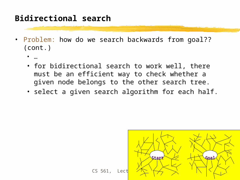
Bidirectional search
• Problem: how do we search backwards from goal?? (cont.)• …
• for bidirectional search to work well, there must be an efficient way to check whether a given node belongs to the other search tree.
• select a given search algorithm for each half.
GoalGoalStartStart
CS 561, Lectures 3-5 150
Bidirectional search
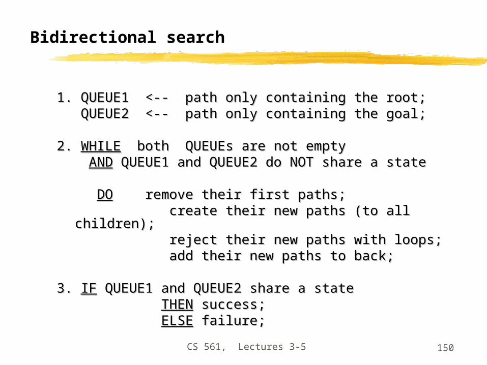
1. QUEUE1 <-- path only containing the root;1. QUEUE1 <-- path only containing the root; QUEUE2 <-- path only containing the goal;QUEUE2 <-- path only containing the goal;
2. 2. WHILEWHILE both QUEUEs are not empty both QUEUEs are not empty ANDAND QUEUE1 and QUEUE2 do NOT share a state QUEUE1 and QUEUE2 do NOT share a state
DODO remove their first paths; remove their first paths; create their new paths (to all children);create their new paths (to all children); reject their new paths with loops;reject their new paths with loops; add their new paths to back;add their new paths to back;
3. 3. IFIF QUEUE1 and QUEUE2 share a state QUEUE1 and QUEUE2 share a state THENTHEN success; success; ELSEELSE failure; failure;

CS 561, Lectures 3-5 151
Bidirectional search
• Completeness: Yes,
• Time complexity: 2*O(b d/2) = O(b d/2) • Space complexity: O(b m/2) • Optimality: Yes
• To avoid one by one comparison, we need a hash table of size O(b m/2)
• If hash table is used, the cost of comparison is O(1)

CS 561, Lectures 3-5 152
Bidirectional Search
d
d / 2
Initial State Final State

CS 561, Lectures 3-5 153
Bidirectional search
• Bidirectional search merits:• Big difference for problems with branching
factor b in both directions• A solution of length d will be found in O(2bd/2) = O(bd/2)• For b = 10 and d = 6, only 2,222 nodes are needed
instead of 1,111,111 for breadth-first search

CS 561, Lectures 3-5 154
Bidirectional search
• Bidirectional search issues• Predecessors of a node need to be generated
• Difficult when operators are not reversible
• What to do if there is no explicit list of goal states?
• For each node: check if it appeared in the other search
• Needs a hash table of O(bd/2)
• What is the best search strategy for the two searches?

CS 561, Lectures 3-5 155
Comparing uninformed search strategies
Criterion Breadth- UniformDepth- Depth- Iterative Bidirectional
first cost first limited deepening (if applicable)
Time b^d b^d b^m b^l b^d b^(d/2)
Space b^d b^d bm bl bd b^(d/2)
Optimal? Yes Yes No No Yes Yes
Complete? Yes Yes No Yes, Yes Yesif ld
• b – max branching factor of the search tree• d – depth of the least-cost solution• m – max depth of the state-space (may be infinity)• l – depth cutoff
CS 561, Lectures 3-5 156
Summary
• Problem formulation usually requires abstracting away real-world details to define a state space that can be explored using computer algorithms.
• Once problem is formulated in abstract form, complexity analysis helps us picking out best algorithm to solve problem.
• Variety of uninformed search strategies; difference lies in method used to pick node that will be further expanded.
• Iterative deepening search only uses linear space and not much more time than other uniformed search strategies.