Embed Size (px)
Citation preview
1
CS 536 – Density Estimation - Clustering - 1
CS 536: Machine Learning
Nonparametric Density EstimationUnsupervised Learning - Clustering
Fall 2005Ahmed Elgammal
Dept of Computer ScienceRutgers University
CS 536 – Density Estimation - Clustering - 2
Outlines
• Density estimation• Nonparametric kernel density estimation• Mixture Densities• Unsupervised Learning - Clustering:
– Hierarchical Clustering– K-means Clustering– Mean Shift Clustering– Spectral Clustering – Graph Cuts– Application to Image Segmentation
2
CS 536 – Density Estimation - Clustering - 3
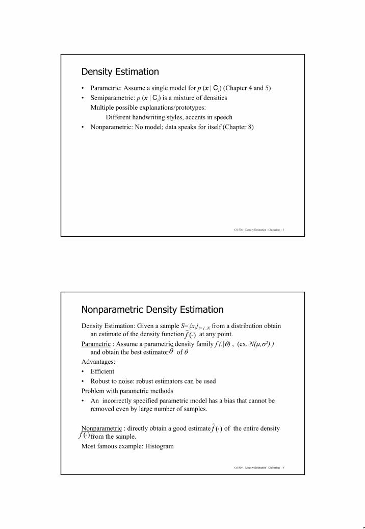
Density Estimation
• Parametric: Assume a single model for p (x | Ci) (Chapter 4 and 5)• Semiparametric: p (x | Ci) is a mixture of densities
Multiple possible explanations/prototypes:Different handwriting styles, accents in speech
• Nonparametric: No model; data speaks for itself (Chapter 8)
CS 536 – Density Estimation - Clustering - 4
Nonparametric Density Estimation
Density Estimation: Given a sample S={xi}i=1..N from a distribution obtain an estimate of the density function at any point.
Parametric : Assume a parametric density family f (.|θ) , (ex. N(µ,σ2) ) and obtain the best estimator of θ
Advantages:• Efficient• Robust to noise: robust estimators can be usedProblem with parametric methods• An incorrectly specified parametric model has a bias that cannot be
removed even by large number of samples.
Nonparametric : directly obtain a good estimate of the entire densityfrom the sample.
Most famous example: Histogram
θ)
)(⋅f)
)(⋅f
)(⋅f)
3
CS 536 – Density Estimation - Clustering - 5
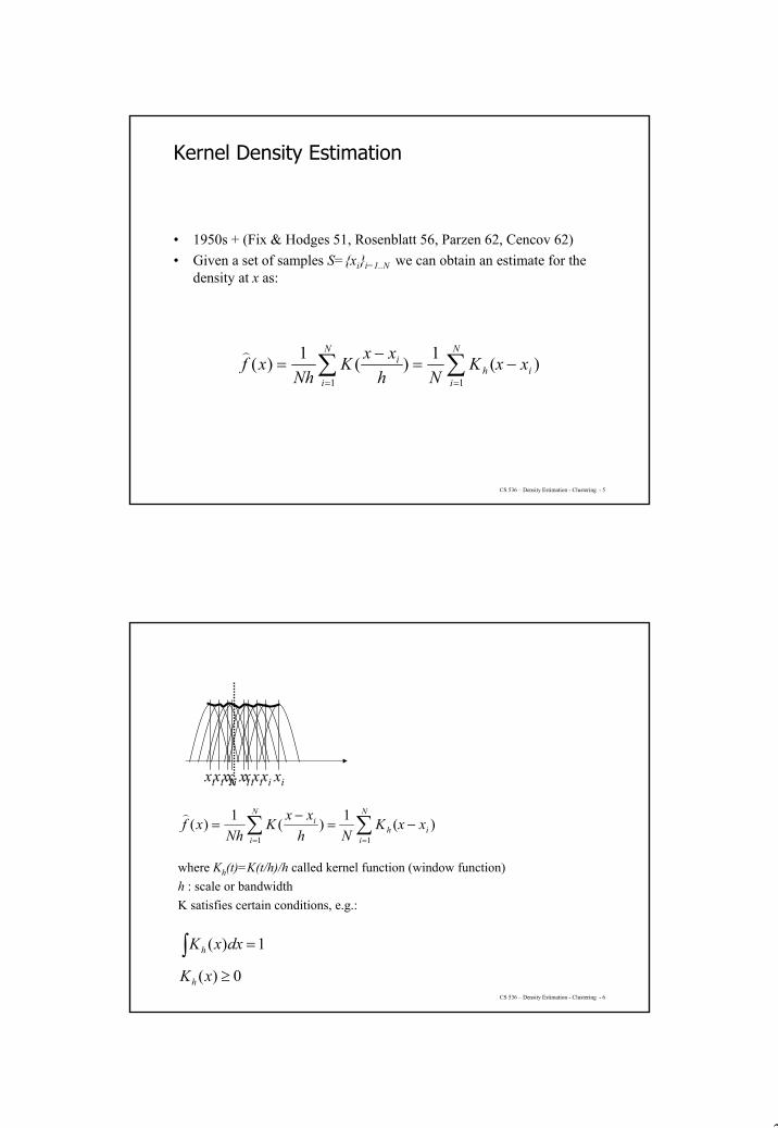
Kernel Density Estimation
• 1950s + (Fix & Hodges 51, Rosenblatt 56, Parzen 62, Cencov 62)• Given a set of samples S={xi}i=1..N we can obtain an estimate for the
density at x as:
)(1)(1)(11
i
N
ih
N
i
i xxKNh
xxKNh
xf −=−
= ∑∑==
)
CS 536 – Density Estimation - Clustering - 6
where Kh(t)=K(t/h)/h called kernel function (window function)h : scale or bandwidthK satisfies certain conditions, e.g.:
xxi xixi xi xixi xi xixi
)(1)(1)(11
i
N
ih
N
i
i xxKNh
xxKNh
xf −=−
= ∑∑==
)
0)( ≥xKh
∫ =1)( dxxKh
4
CS 536 – Density Estimation - Clustering - 7
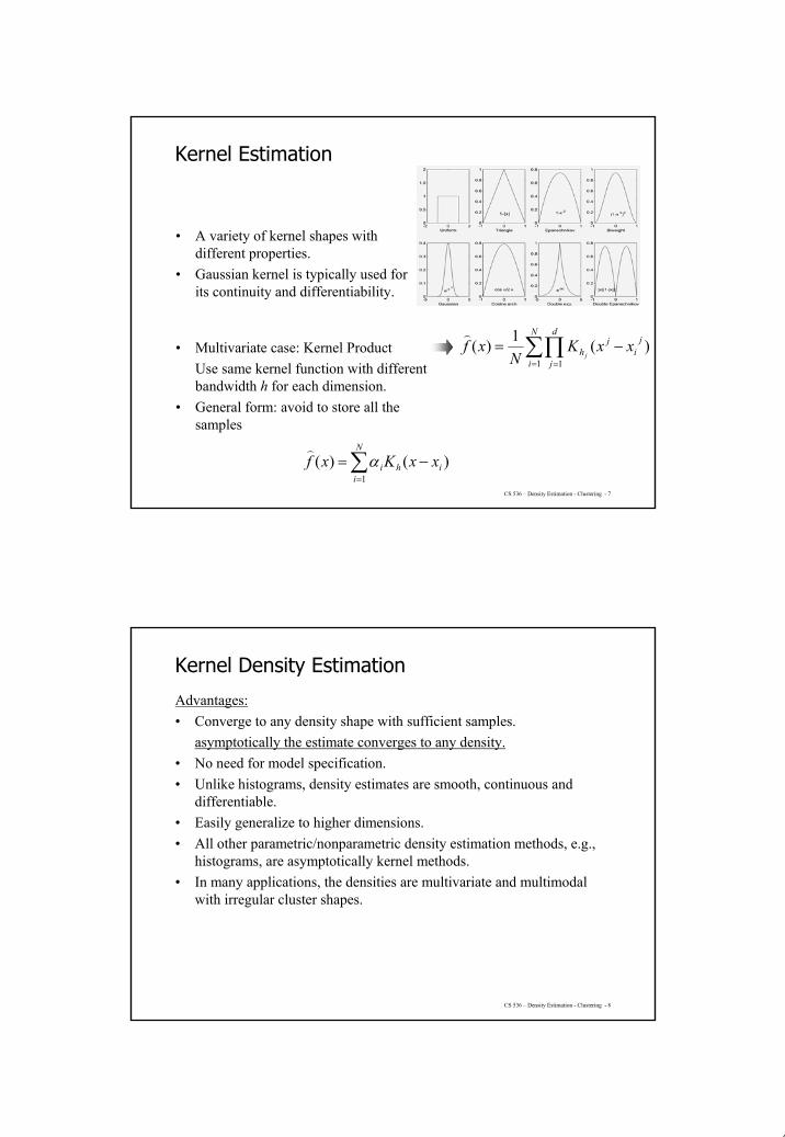
Kernel Estimation
• A variety of kernel shapes with different properties.
• Gaussian kernel is typically used for its continuity and differentiability.
• Multivariate case: Kernel Product Use same kernel function with different bandwidth h for each dimension.
• General form: avoid to store all the samples
∑∏= =
−=N
i
d
j
ji
jh xxK
Nxf
j1 1
)(1)()
∑=
−=N
iihi xxKxf
1)()( α
)
CS 536 – Density Estimation - Clustering - 8
Kernel Density Estimation
Advantages:• Converge to any density shape with sufficient samples.
asymptotically the estimate converges to any density.• No need for model specification.• Unlike histograms, density estimates are smooth, continuous and
differentiable.• Easily generalize to higher dimensions.• All other parametric/nonparametric density estimation methods, e.g.,
histograms, are asymptotically kernel methods.• In many applications, the densities are multivariate and multimodal
with irregular cluster shapes.

5
CS 536 – Density Estimation - Clustering - 9
Example: color clusters• Cluster shapes are irregular • Cluster boundaries are not well defined.
rom omaniciu and eer ean shift robustapproach toward feature space analysis
CS 536 – Density Estimation - Clustering - 10
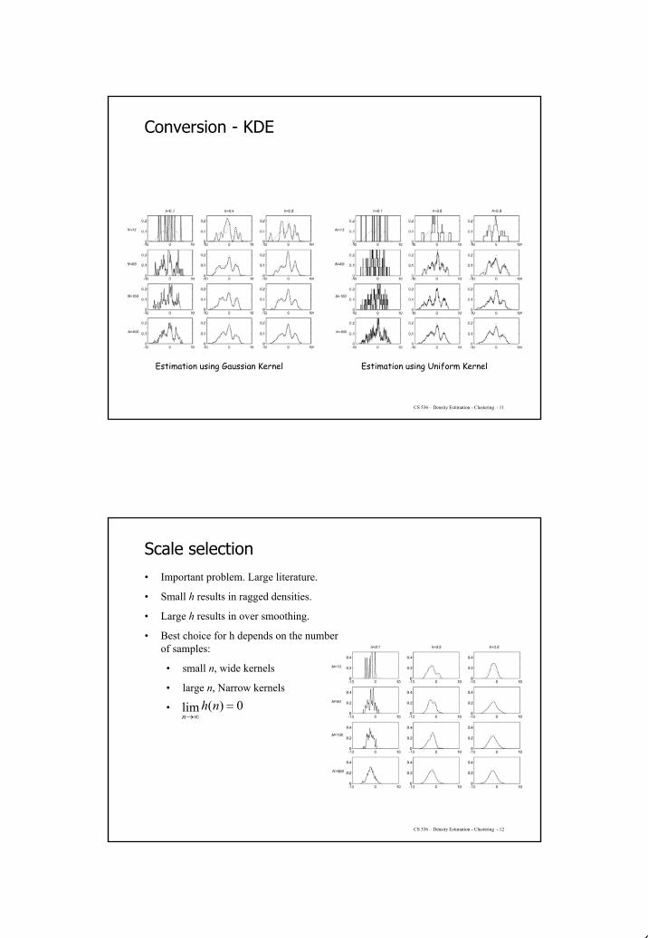
Conversion - KDE
Estimation using Gaussian Kernel Estimation using Uniform Kernel
6
CS 536 – Density Estimation - Clustering - 11
Conversion - KDE
Estimation using Gaussian Kernel Estimation using Uniform Kernel
CS 536 – Density Estimation - Clustering - 12
Scale selection• Important problem. Large literature.
• Small h results in ragged densities.
• Large h results in over smoothing.
• Best choice for h depends on the number of samples:
• small n, wide kernels
• large n, Narrow kernels
• 0)(lim =∞→
nhn
7
CS 536 – Density Estimation - Clustering - 13
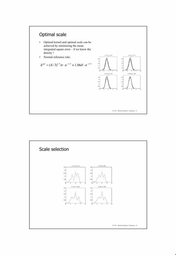
Optimal scale• Optimal kernel and optimal scale can be
achieved by minimizing the mean integrated square error – if we know the density !
• Normal reference rule:
5/15/15/1 ˆ06.1)3/4( −− ⋅≈⋅= nnhopt σσ
CS 536 – Density Estimation - Clustering - 14
Scale selection

8
CS 536 – Density Estimation - Clustering - 15
From R. O. Duda, P. E. Hart, and D. G. Stork. “Pattern Classification” Wiley, New York, 2nd edition, 2000
CS 536 – Density Estimation - Clustering - 16
Density Estimation
• Parametric: Assume a single model for p (x | Ci) (Chapter 4 and 5)• Semiparametric: p (x | Ci) is a mixture of densities
Multiple possible explanations/prototypes:Different handwriting styles, accents in speech
• Nonparametric: No model; data speaks for itself (Chapter 8)
9
CS 536 – Density Estimation - Clustering - 17
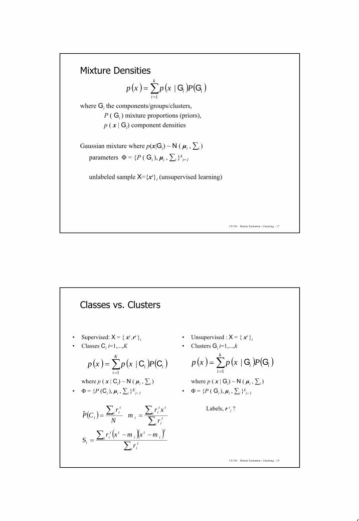
Mixture Densities
where Gi the components/groups/clusters, P ( Gi ) mixture proportions (priors),p ( x | Gi) component densities
Gaussian mixture where p(x|Gi) ~ N ( µi , ∑i )
parameters Φ = {P ( Gi ), µi , ∑i }ki=1
unlabeled sample X={xt}t (unsupervised learning)
( ) ( ) ( )∑=
=k
iii Ppp
1| GGxx
CS 536 – Density Estimation - Clustering - 18
Classes vs. Clusters
• Supervised: X = { xt ,rt }t
• Classes Ci i=1,...,K
where p ( x | Ci) ~ N ( µi , ∑i ) • Φ = {P (Ci ), µi , ∑i }K
i=1
• Unsupervised : X = { xt }t
• Clusters Gi i=1,...,k
where p ( x | Gi) ~ N ( µi , ∑i ) • Φ = {P ( Gi ), µi , ∑i }k
i=1
Labels, r ti ?
( ) ( ) ( )∑=
=k
iii Ppp
1| GGxx( ) ( ) ( )∑
=
=K
iii Ppp
1| CCxx
( )
( )( )∑
∑∑∑∑
−−=
==
tt
i
Ti
tt i
tti
i
tt
i
ttt
ii
tt
ii
rr
rr
Nr
CP̂
mxmx
xm
S

10
CS 536 – Density Estimation - Clustering - 19
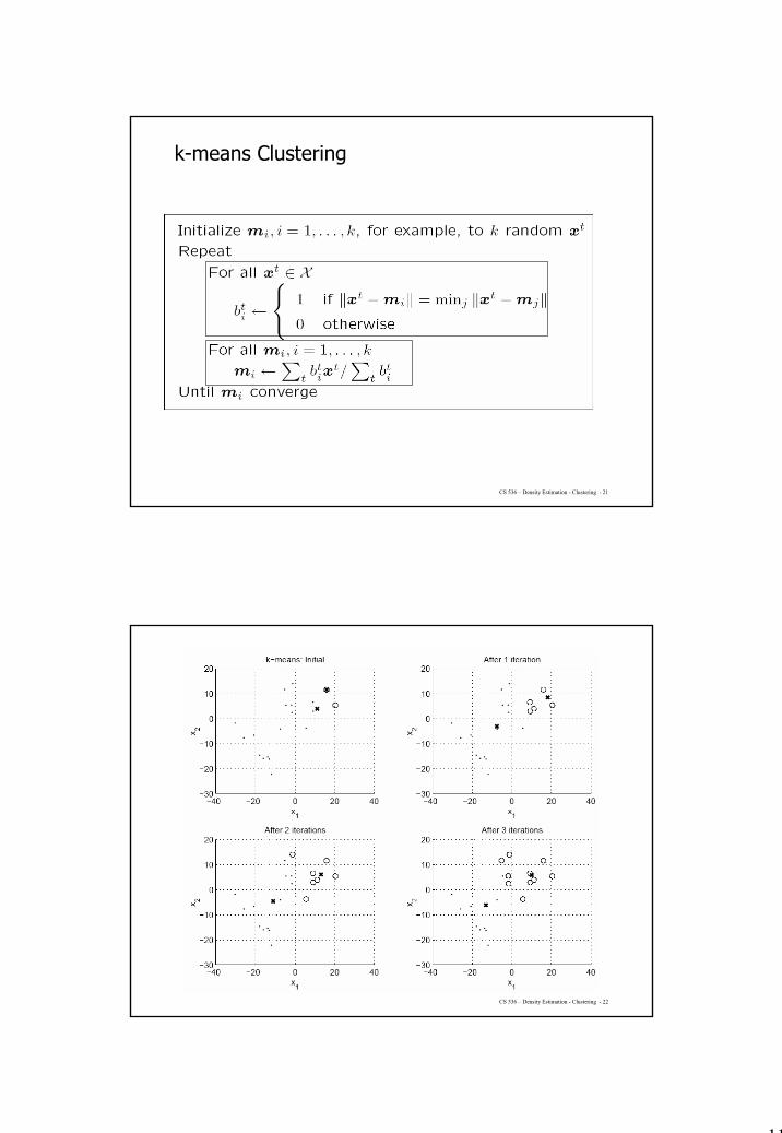
k-Means Clustering
• Find k reference vectors (prototypes/codebook vectors/codewords) whichbest represent data
• Reference vectors, mj, j =1,...,k• Use nearest (most similar) reference:
• Reconstruction error
jt
jit mxmx −=− min
{ }( )
−=−
=
−= ∑ ∑=
otherwise0minif 1
1
jt
jit
ti
t i itt
ikii
b
bE
mxmx
mxm X
CS 536 – Density Estimation - Clustering - 20
Encoding/Decoding
−=−
= otherwise0minif 1 j
t
jit
tib mxmx
11
CS 536 – Density Estimation - Clustering - 21
k-means Clustering
CS 536 – Density Estimation - Clustering - 22
12
CS 536 – Density Estimation - Clustering - 23
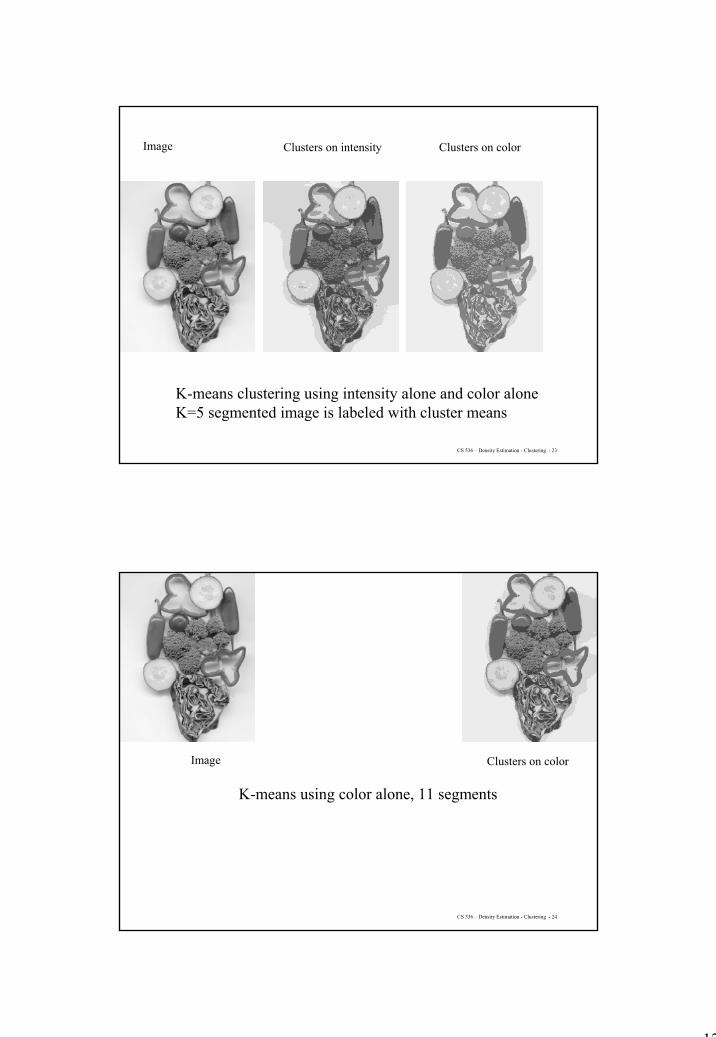
K-means clustering using intensity alone and color aloneK=5 segmented image is labeled with cluster means
Image Clusters on intensity Clusters on color
CS 536 – Density Estimation - Clustering - 24
K-means using color alone, 11 segments
Image Clusters on color
13
CS 536 – Density Estimation - Clustering - 25
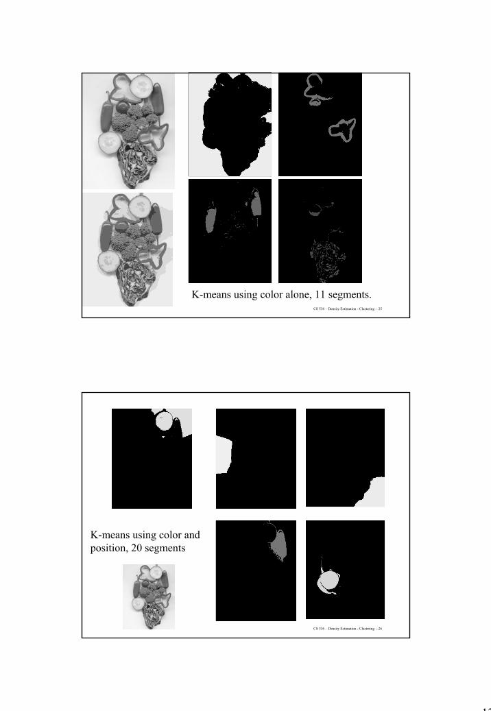
K-means using color alone, 11 segments.
CS 536 – Density Estimation - Clustering - 26
K-means using color andposition, 20 segments
14
CS 536 – Density Estimation - Clustering - 27
Hierarchical Clustering
• Cluster based on similarities/distances• Distance measure between instances xr and xs
Minkowski (Lp) (Euclidean for p = 2)
City-block distance
( ) ( )[ ] pd
j
psj
rj
srm xxd
/1
1, ∑ =
−=xx
( ) ∑ =−=
d
jsj
rj
srcb xxd
1,xx
CS 536 – Density Estimation - Clustering - 28
Hierarchical Clustering:
• Agglomerative clustering – clustering by merging – bottom-up– Each data point is assumed to be a cluster– Recursively merge clusters– Algorithm:
• Make each point a separate cluster• Until the clustering is satisfactory
– Merge the two clusters with the smallest inter-cluster distance
• Divisive clustering – clustering by splitting – top-down– The entire data set is regarded as a cluster– Recursively split clusters– Algorithm:
• Construct a single cluster containing all points• Until the clustering is satisfactory
– Split the cluster that yields the two components with the largest inter-cluster distance
15
CS 536 – Density Estimation - Clustering - 29
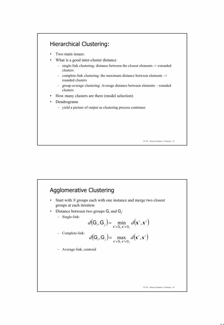
Hierarchical Clustering:
• Two main issues:• What is a good inter-cluster distance
– single-link clustering: distance between the closest elements -> extended clusters
– complete-link clustering: the maximum distance between elements –> rounded clusters
– group-average clustering: Average distance between elements – rounded clusters
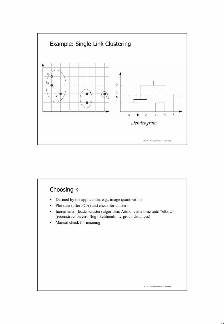
• How many clusters are there (model selection)• Dendrograms
– yield a picture of output as clustering process continues
CS 536 – Density Estimation - Clustering - 30
Agglomerative Clustering
• Start with N groups each with one instance and merge two closest groups at each iteration
• Distance between two groups Gi and Gj:– Single-link:
– Complete-link:
– Average-link, centroid
( ) ( )srji dd
js
ir
xxxx
,min,, GG
GG∈∈
=
( ) ( )srji dd
js
ir
xxxx
,max,, GG
GG∈∈
=
16
CS 536 – Density Estimation - Clustering - 31
Dendrogram
Example: Single-Link Clustering
CS 536 – Density Estimation - Clustering - 32
Choosing k
• Defined by the application, e.g., image quantization• Plot data (after PCA) and check for clusters• Incremental (leader-cluster) algorithm: Add one at a time until “elbow”
(reconstruction error/log likelihood/intergroup distances)• Manual check for meaning
17
CS 536 – Density Estimation - Clustering - 33
CS 536 – Density Estimation - Clustering - 34
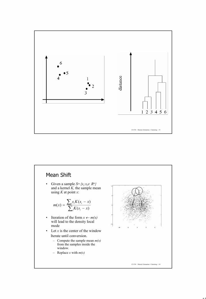
Mean Shift• Given a sample S={si:si∈ Rn}
and a kernel K, the sample mean using K at point x:
• Iteration of the form x ← m(x)will lead to the density local mode
• Let x is the center of the windowIterate until conversion.
– Compute the sample mean m(x)from the samples inside the window.
– Replace x with m(x)
∑∑
−
−=
i i
i ii
xsKxsKs
xm)()(
)(
18
CS 536 – Density Estimation - Clustering - 35
Mean Shift
• Given a sample S={si:si∈ Rn} and a kernel K, the sample mean using Kat point x:
• Fukunaga and Hostler 1975 introduced the mean shift as the difference m(x)-x using a flat kernel.
• Iteration of the form x ← m(x) will lead to the density mode• Cheng 1995 generalized the definition using general kernels and
weighted data
• Recently popularized by D. Comaniciu and P. Meer 99+• Applications: Clustering[Cheng,Fu 85], image filtering,
segmentation[Meer 99] and tracking [Meer 00].
∑∑
−
−=
i i
i ii
xsKxsKs
xm)()(
)(
)()()()(
)(ii i
i iii
swxsKswxsKs
xm∑∑
−
−=
CS 536 – Density Estimation - Clustering - 36
Mean Shift
• Iterations of the form x ← m(x) are called mean shift algorithm.• If K is a Gaussian (e.g.) and the density estimate using K is
• Using Gaussian Kernel Kσ(x), the derivative is we can show that:
• the mean shift is in the gradient direction of the density estimate.
∑ −=i ii swsxKCxP )()()(ˆ
xxmxPxP
−=∇ )(
)(ˆ)(ˆ
)()( 2 xKxxK σσ σ−=′
19
CS 536 – Density Estimation - Clustering - 37
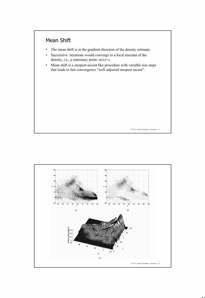
Mean Shift
• The mean shift is in the gradient direction of the density estimate. • Successive iterations would converge to a local maxima of the
density, i.e., a stationary point: m(x)=x .• Mean shift is a steepest-ascent like procedure with variable size steps
that leads to fast convergence “well-adjusted steepest ascent”.
CS 536 – Density Estimation - Clustering - 38
20
CS 536 – Density Estimation - Clustering - 39
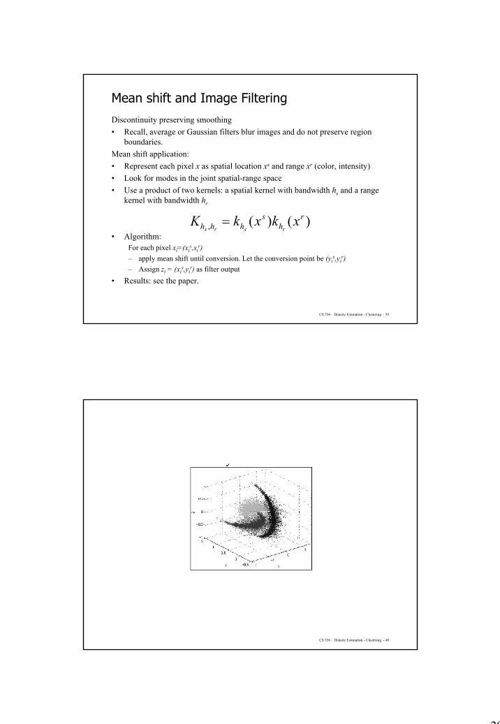
Mean shift and Image FilteringDiscontinuity preserving smoothing• Recall, average or Gaussian filters blur images and do not preserve region
boundaries.Mean shift application:• Represent each pixel x as spatial location xs and range xr (color, intensity)• Look for modes in the joint spatial-range space• Use a product of two kernels: a spatial kernel with bandwidth hs and a range
kernel with bandwidth hr
• Algorithm: For each pixel xi=(xi
s,xir)
– apply mean shift until conversion. Let the conversion point be (yis,yi
r)– Assign zi = (xi
s,yir) as filter output
• Results: see the paper.
)()(,r
hs
hhh xkxkKrsrs
=
CS 536 – Density Estimation - Clustering - 40

21
CS 536 – Density Estimation - Clustering - 42
What is a Graph Cut:• We have undirected, weighted graph G=(V,E)• Remove a subset of edges to partition the graph into two disjoint sets
of vertices A,B (two sub graphs):A ∪ B = V, A ∩ B = Φ
Graph Cut
CS 536 – Density Estimation - Clustering - 43
• Each cut corresponds to some cost (cut): sum of the weights for the edges that have been removed.
Graph Cut
∑∈∈
=BvAu
vuwBAcut,
),(),(
A B
22
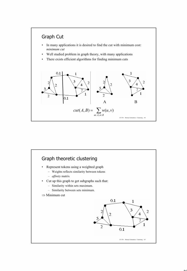
CS 536 – Density Estimation - Clustering - 44
• In many applications it is desired to find the cut with minimum cost: minimum cut
• Well studied problem in graph theory, with many applications• There exists efficient algorithms for finding minimum cuts
Graph Cut
∑∈∈
=BvAu
vuwBAcut,
),(),(
A B
CS 536 – Density Estimation - Clustering - 45
Graph theoretic clustering
• Represent tokens using a weighted graph– Weights reflects similarity between tokens– affinity matrix
• Cut up this graph to get subgraphs such that:– Similarity within sets maximum.– Similarity between sets minimum.
⇒ Minimum cut
23
CS 536 – Density Estimation - Clustering - 46
CS 536 – Density Estimation - Clustering - 47
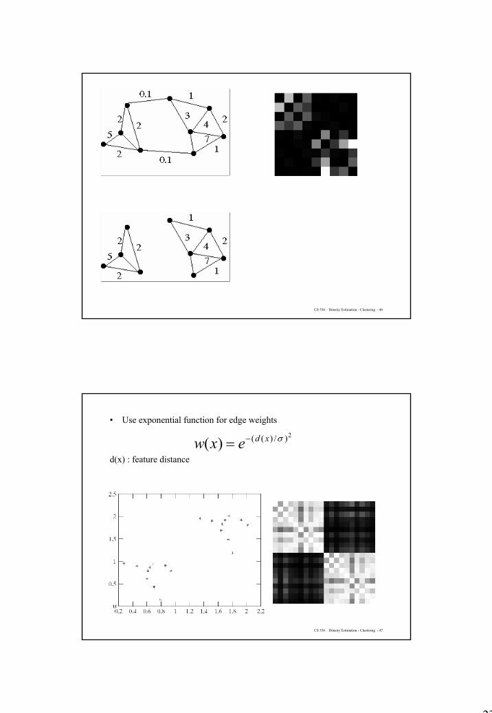
• Use exponential function for edge weights
d(x) : feature distance
2)/)(()( σxdexw −=

24
CS 536 – Density Estimation - Clustering - 48
Scale affects affinity
σ=0.1 σ=0.2 σ=1
2)/)(()( σxdexw −=
CS 536 – Density Estimation - Clustering - 49
Eigenvectors and clustering• Simplest idea: we want a vector w
giving the association between each element and a cluster
• We want elements within this cluster to, on the whole, have strong affinity with one another
• We could maximize
nTn Aww
Association of element i with cluster n ×Affinity between i and j ×
Association of element j with cluster n
Sum of
w
25
CS 536 – Density Estimation - Clustering - 50
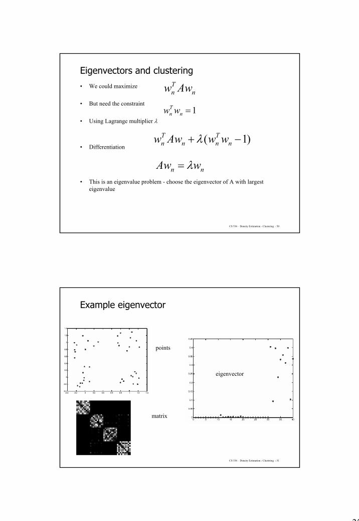
Eigenvectors and clustering• We could maximize
• But need the constraint
• Using Lagrange multiplier λ
• Differentiation
• This is an eigenvalue problem - choose the eigenvector of A with largest eigenvalue
nTn Aww
1=nTn ww
)1( −+ nTnn
Tn wwAww λ
nn wAw λ=
CS 536 – Density Estimation - Clustering - 51
Example eigenvector
points
matrix
eigenvector
26
CS 536 – Density Estimation - Clustering - 52
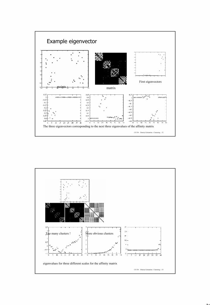
Example eigenvector
points matrix
The three eigenvectors corresponding to the next three eigenvalues of the affinity matrix
First eigenvectors
CS 536 – Density Estimation - Clustering - 53
eigenvalues for three different scales for the affinity matrix
More obvious clustersToo many clusters !

27
CS 536 – Density Estimation - Clustering - 54
More than two segments
• Two options– Recursively split each side to get a tree, continuing till the eigenvalues are
too small– Use the other eigenvectors
Algorithm• Construct an Affinity matrix A• Computer the eigenvalues and eigenvectors of A• Until there are sufficient clusters
– Take the eigenvector corresponding to the largest unprocessed eigenvalue; zero all components for elements already clustered, and threshold the remaining components to determine which element belongs to this cluster, (you can choose a threshold by clustering the components, or use a fixed threshold.)
– If all elements are accounted for, there are sufficient clusters
CS 536 – Density Estimation - Clustering - 55
We can end up with eigenvectors that do not split clusters because any linear combination of eigenvectors with the same eigenvalue is also an eigenvector.
28
CS 536 – Density Estimation - Clustering - 73
Sources
• R. O. Duda, P. E. Hart, and D. G. Stork. “Pattern Classification.”Wiley, New York, 2nd edition, 2000
• Ethem Alpaydin “Introduction to Machine Learning” Chapter 7• Forsyth and Ponce, Computer Vision a Modern approach: chapter 14:
14.1,14.2,14.4.• Slides by
– D. Forsyth @ Berkeley
• Slides by Ethem Alpaydin