CS 476 (Winter 2014 - 1141) - GitHub Pages

Winter 2014 TABLE OF CONTENTS

CS 476 (Winter 2014 - 1141)Numerical Computation for Financial ModelingProf. P.A. ForsythUniversity of Waterloo

LATEXer: W. KONG

http://wwkong.github.io

Last Revision: April 30, 2014

Table of Contents1 Introduction 1

1.1 Financial Terminology . . . . . . . . . . . . . . . . . . . . . . . . . . . . . . . . . . . . . . . . . . . . . . . . . 11.2 Arbitrage . . . . . . . . . . . . . . . . . . . . . . . . . . . . . . . . . . . . . . . . . . . . . . . . . . . . . . . . 21.3 Hedging . . . . . . . . . . . . . . . . . . . . . . . . . . . . . . . . . . . . . . . . . . . . . . . . . . . . . . . . . 2

2 Stochastic Calculus in Finance 32.1 Brownian Motion . . . . . . . . . . . . . . . . . . . . . . . . . . . . . . . . . . . . . . . . . . . . . . . . . . . . 32.2 Properties of Brownian Motion . . . . . . . . . . . . . . . . . . . . . . . . . . . . . . . . . . . . . . . . . . . . 42.3 Ito’s Lemma . . . . . . . . . . . . . . . . . . . . . . . . . . . . . . . . . . . . . . . . . . . . . . . . . . . . . . . 42.4 Black-Scholes Equation . . . . . . . . . . . . . . . . . . . . . . . . . . . . . . . . . . . . . . . . . . . . . . . . . 62.5 Hedging in Continuous Time . . . . . . . . . . . . . . . . . . . . . . . . . . . . . . . . . . . . . . . . . . . . . 7

3 Computational Methods 73.1 Lattice Model for Pricing . . . . . . . . . . . . . . . . . . . . . . . . . . . . . . . . . . . . . . . . . . . . . . . . 83.2 Dynamic Programming . . . . . . . . . . . . . . . . . . . . . . . . . . . . . . . . . . . . . . . . . . . . . . . . . 83.3 Risk Neutral World . . . . . . . . . . . . . . . . . . . . . . . . . . . . . . . . . . . . . . . . . . . . . . . . . . . 93.4 Monte Carlo . . . . . . . . . . . . . . . . . . . . . . . . . . . . . . . . . . . . . . . . . . . . . . . . . . . . . . . 103.5 Measuring Risk . . . . . . . . . . . . . . . . . . . . . . . . . . . . . . . . . . . . . . . . . . . . . . . . . . . . . 123.6 Hedging Portfolios . . . . . . . . . . . . . . . . . . . . . . . . . . . . . . . . . . . . . . . . . . . . . . . . . . . 12

Delta-Gamma Hedging . . . . . . . . . . . . . . . . . . . . . . . . . . . . . . . . . . . . . . . . . . . . . . . . 14Delta-Vega Hedging . . . . . . . . . . . . . . . . . . . . . . . . . . . . . . . . . . . . . . . . . . . . . . . . . . . 14

3.7 Random Number Generation . . . . . . . . . . . . . . . . . . . . . . . . . . . . . . . . . . . . . . . . . . . . . 143.8 Efficiency of Algorithms . . . . . . . . . . . . . . . . . . . . . . . . . . . . . . . . . . . . . . . . . . . . . . . . 173.9 Correlated Random Numbers . . . . . . . . . . . . . . . . . . . . . . . . . . . . . . . . . . . . . . . . . . . . . 173.10 Hedging Parameters . . . . . . . . . . . . . . . . . . . . . . . . . . . . . . . . . . . . . . . . . . . . . . . . . . 19

4 Partial Differential Equations 194.1 Finite Difference Approximations . . . . . . . . . . . . . . . . . . . . . . . . . . . . . . . . . . . . . . . . . . . 204.2 Discretization Methods for PDEs . . . . . . . . . . . . . . . . . . . . . . . . . . . . . . . . . . . . . . . . . . . . 20

5 Stability 225.1 Positive Coefficients . . . . . . . . . . . . . . . . . . . . . . . . . . . . . . . . . . . . . . . . . . . . . . . . . . 225.2 Crank-Nicholson Method . . . . . . . . . . . . . . . . . . . . . . . . . . . . . . . . . . . . . . . . . . . . . . . . 245.3 Von-Neumann Analysis . . . . . . . . . . . . . . . . . . . . . . . . . . . . . . . . . . . . . . . . . . . . . . . . . 25

6 Lattice vs. Finite Difference Methods 25

These notes are currently a work in progress, and as such may be incomplete or contain errors.

i

http://wwkong.github.io

Winter 2014 ACKNOWLEDGMENTS

ACKNOWLEDGMENTS:Special thanks to Michael Baker and his LATEX formatted notes. They were the inspiration for the structure of these notes.

ii

Winter 2014 ABSTRACT

Abstract

The purpose of these notes is to provide the reader with a secondary reference to the material covered in CS 476. The

formal prerequisite to this course is CS 371/AMATH 242/CM 271 but this author believes that the overlap between the two

courses is less than 30%. Readers should have a good background in linear algebra, basic statistics, and calculus before

enrolling in this course.

iii

Winter 2014 1 INTRODUCTION

Errata

User ID: cs476_user_2014

Pass: cs476!2014

url: www.student.cs.uwaterloo.ca/~cs476

(Used to download the slides)

1 Introduction

The following are just notes regarding the slides in the first lecture.

• Take note of the GBM formula in slide 7 of the this lecture

• Definition of a hedged portfolio is found in slide 10 of this lecture

– Hedinging objective: dΠ = Π(t+ dt)−Π(t) = 0

– Under the Black-Scholes equation, the optimal units of the underlying asset in a hedged portfolio is e = ∂V∂S

• The no-arbitrage value of an option is the cost of setting up the hedged portfolio

• In reality, the bid-ask spread is composed of (profit + compensation for imperfect hedge)

• Problems with GBM?

– Jump diffusion (1976, slide 24 of this lecture); Black Swans

• Jump diffusion adds the term (J − 1) dq to GBM

We now can proceed to some basic terminology.

1.1 Financial Terminology

Consider a European put/call at some time T in the future. The holder has the right but not the obligation to buy (sell) theunderlying risky asset at some strike price K. The right to buy is given for a call and the right to sell is given for a put. Thepayoffs of a call and put are respectively

max(S −K, 0) = (S −K)+

max(K − S, 0) = (K − S)+

Example 1.1. Suppose a stock today has price S0 and in 3 months it has two values Su = 22 and Sd = 18. For a Europeancall of K = 21, the value 3 months later is Vu = 1 and Vd = 0. If pu = 0.1 and pd = 0.9, then the EPV is

(0.1× 1 + 0.9× 0)e−r4t

If the risk free rate is 12% and the time unit is 1 year, then the EPV is 0.097. Suppose that someone offers to buy this optionfor 0.3. From your point of view, you might expect to profit 0.2, but the other person claims there is an arbitrage opportunity.

Definition 1.1. As an aside, an arbitrage opportunity exists if, starting from zero initial wealth, an investor can devise astrategy such that (i) there exists a zero probability of loss (ii) there is a positive probability of gain.

1

Winter 2014 1 INTRODUCTION

1.2 Arbitrage

Definition 1.2. The risk-free rate of return is the return earned by an investment with zero risk.

Example 1.2. An example of a risk-free asset is a government bond. Note that if a portfolio does not earn the risk-free ratethen there is an arbitrage opportunity (via shorting/longing the portfolio and buying/selling at the risk free rate). Supplyand demand effects (the demand for the portfolio would decrease/increase with return increasing/decreasing) would thennormalize the return of the portfolio and push it towards the risk free rate.

Corollary 1.1. (No-arbitrage Rule #1) A portfolio which is risk free must earn the risk free rate.

Definition 1.3. A short position is constructed by borrowing an asset we don’t own, selling it, but we have to give it back inthe future. If you short it, then mathematically you own a negative quantity.

Continuing from the previous example, instead of examining expected values we use the following idea (1) we will constructa portfolio which has no uncertainty in 3 months (2) since the portfolio is risk free, it must earn the risk free rate. To do this,we construct the portfolio:

Π = δS − V

where S is the stock and V is the option. So we compute δ such that Π has a certain value in 3 months. The two possiblevalues are Πu = 22δ − 1 and Πd = 18δ and setting Πu = Πd we get δ = 1/4 and the value being 4.50. The value, discountingat the risk-free rate, is 4.50e0.12×0.25 = 4.367. With S0 = 20 and δ = 1/4, the value of V0 can be solved to be V0 = 0.633.

We claim that this no-arbitrage price should be the market price. To see this, suppose the price in the market was more than0.633. The we do the following:

1. Borrow from bank and construct the portfolio Π = −V + δS (buy stock, sell one call)

2. In 3 months, sell stock, pay off option holder, and pay back the bank loan

3. Profit

Conversely, if the option sells for less than 0.633, the we do the following:

1. Deposit into bank and construct the portfolio Π = V − δS (short stock, buy one call)

2. In 3 months, use the cash in the bank to buy back the stock, liquidate the short, and take the gain in the option

3. Profit

In both cases, this is a money machine and gains are only limited by borrowing. Note that the no-arbitrage price is indepen-dent of p1 and p2.

1.3 Hedging

Example 1.3. Here is an example of a hedge using the previous section’s main example. Suppose that I sell a call and wantto completely hedge the risk where we have S0 = 20, Su = 22, Sd = 18, K = 21, r = 12%, and T = 3 months. This is thestrategy:

1. Sell option for 0.633

2. Borrow 4.367 from the bank which means we have to pay back 4.50 in 3 months

3. Buy 1/4 of share of stock at S0 = 20

4. If S1/4 = Su then we have 5.5 in equities so we sell the stock, pay back the option at 1 and pay back the bank loan at4.5 to get a profit of 0

5. If S1/4 = Sd then we have 4.5 in equities so we sell the stock, do not pay back the option (value is 0) and

Of course, no one would want to do this since there is no gain. Usually, we have the effects of the bid-ask spread. The askprice is usually the higher one.

2

Winter 2014 2 STOCHASTIC CALCULUS IN FINANCE

2 Stochastic Calculus in Finance

In computational finance, we do not attempt to predict stock prices since they are stochastic. However, there are otherapplications.

2.1 Brownian Motion

Definition 2.1. A Brownian motion with drift is specified as follows. Suppose that X is a random variable and take t tot+ dt and X to X + dX. We model dX and dZ as

dX = α︸︷︷︸(1)

dt+

(2)︷︸︸︷σ × dZ︸︷︷︸

(3)

, dZ = φ√dt

where φ ∼ N(0, 1), (1) is the drift (2) is the volatility, (3) is the increment of a Wiener process, and

E[dX] = E[α · dt] + E[σdZ] = α dt+ 0

V ar[dX] = E[(dX − E[dx])2] = E[σ2dZ2] = σ2 dt

We can model Brownian motion using something called a lattice model (binomial tree). Let X(t) be the position of aparticle at time t. At t = 0, X = X0 and after an interval 4t, t1 = t0 +4t with X0 7→ X0 +4h (under probability p) andX0 7→ X0 − 4h (under probability q = 1 − p). We are assuming that X follows a Markov process; that is, the probabilitydistribution of future positions depends on where we are now. Under this structure, we have

E[4Xi] = (p− q) · 4hE[4X2

i ] = p(4h)2 + q(−4h)2 = (4h)2

V ar[4Xi] = E[4X2i ]− (E[4Xi])

2 = 4pq(4h)2

Consider some finite time t where the total number of moves is n = t/4t. If Xi = X(ti) then

E[(4Xi − E[4Xi])(4Xj − E[4Xj ])] = Cov(4Xi,4Xj) =i 6=j

0

We also have the property that

E[Xn −X0] = E

[n−1∑i=1

4Xi

]=∑i

(p− q)4h = n(p− q)4h =t(p− q)4h4t

(1) V ar[Xn −X0] =∑i

V ar[4Xi] =t(4pq(4h)2)

4t

From here, we plan to take some limits: 4t → 0 and simultaneously n → ∞, 4t → 0. We first make a few intuitiveassumptions:

lim4t→0

pq 6= 0, lim4t→0

pq = O(1)

Now if (1) is finite and non-zero as 4t→ 0 then(2) 4h = C1

√t

where C1 is independent of 4t. Substituting (2) into the Xn −X0 equations, we get

(3) E[Xn −X0] =t(p− q)4t

· C1

√4t

(4) V ar[Xn −X0] = 4pqtC21

If (3) is independent of 4t as 4t→ 0 then(5) (p− q) = C2

√4t

3


where C2 is also independent of 4t. Putting (5) into (3) gives us

(6) E[Xn −X0] = C1C2t

From (4), using p+ q = 1, we have

(7) p =1 + C2

√4t

2, q =

1− C2

√4t

2

Using (7) in (4) gives us

(8) V ar[Xn −X0] = (1− C224t)C2

1 t4t→0

= C21

Suppose that [Xn −X0] ∼ dx and [t− 0] ∼ dt. Recall E[dX] = α dt, V ar[dX] = σ2 dt and dx = α dt+ σ dZ. Choose C1 = σand C2 = α/σ and remark that this causes the first two moments, (8) and (6), between the SDE and the random walk to bethe same.

The solution of an SDE is the expression for the probability density of the outcome.

It can be shown that the density of the random walk converges to the solution of the SDE.

Summary 1. A discrete random walk on the lattice with the properties

4h = σ√4t, p =

1 + ασ

√t

σ, q = 1− p

converges to the solution of dx = α dt+ σ dZ where dZ = φ√4t and φ ∼ N(0, 1).

2.2 Properties of Brownian Motion

As 4t→ 0, the distance traveled by a particle is |Xi+1 −Xi| = |4h| and the total distance is

n|4Xi| =t

4t|4h| = t

4tσ√t4t→0

= ∞

To reason about this, observe that4X4t

=±σ√4t

4t4t→0

= ±∞

and hence Brownian motion is infinitely jagged on any time scale.

We also may want to ask the question: Why Geometric Brownian Motion (GBM)? Let sd(x) be the standard deviation of x andremark that:

1. Asset prices cannot be negative

2. E[dSS

]= µ dt u E

[S(t+dt)−S(t)

S(t)

]∼ µ dt and so we expect that the return of a stock should not depend on the units

3. sd[S(t)]E[S(t)] ∼

√eσ2t − 1 ∼ eσ2t/2 as t→∞

4. The density of S(t) is generally log-normal and heavily right-skewed

2.3 Ito’s Lemma

Suppose we have the SDE(1) dx = α(x, t) dt+ c(x, t) dZ

We can interpret (1) as

(2) X(t)−X(0) =

� t

0

α(x(s), s) ds+

� t

0

c(x(s), s) dZ(s)

4


Let

4Z(tj) = Z(tj+1)− Z(tj) = Zj+1 − Zj4t = tj+1 − tj

and define the stochastic integral

(3)

� t

0

c(x(s), s) dZ(s) = lim4t→0

N−1∑j=0

c(x(tj), tj)(Zj+1 − Zj)

where N = t/4t and we call this the Ito definition. Note in (3) that we evaluate the first multiplier in the sum on the lefthand point on each interval. Alternatively,

(4)

� t

0

c(x(s), s) dZ(s) = lim4t→0

N−1∑j=0

c(x(tj+ 12), tj+ 1

2)(Zj+1 − Zj)

and we call this the Stratonovich definition. In stochastic calculus, (3) and (4) give different answers. In the latter definition,we are “looking forward” in time which is not what general happens in finance.

Now the latter integral in stochastic, so we need to define something called an Ito integral. This is the basis for using Ito’sLemma where we need to figure out

(5)

� t

0

c(x(s), s) (dZ(s))2

We claim that

(6)

� t

0

c(x(s), s) (dZ(s))2 =

� t

0

c(x(s), s) ds

which in other words,(7) lim

4t→0

∑cj4Z2

j = lim4t→0

∑cj4t

and in shorthand is dZ2 = dt. The proof (in the course notes) is just showing

(8) lim4t→0

E[(∑

cj4Z2j −

∑cj4t

)]= 0

and in the technical proof, we show that if h(t+4t) = g(t) +O(4tn) as 4t→ 0 then for 4t sufficiently small enough, thereexists a c1 such that

(9) |h(t+4t)− g(t)| ≤ c14tn

Suppose that F = F (x, t), t 7→ t dt and F 7→ F dF . Then

(10) dF =∂F

∂tdt+

∂F

∂xdx+

∂2F

∂x2· dx

2

2+ ...

and

(11) (dX)2 = (a dt+ b dz)2

= a2dt2 + 2ab dt dZ + b2dZ2

= b2dt+O((dt)3/2)

and (11), (10), (2) give us

(12) dF = F dt+ Fxdx+ Fxxdx2

2+ ...

= F dt+ Fx(a dt+ b dZ) + Fxx

(1

2

)b2dt+O((dt)3/2)

=

[aFx +

b2

2Fxx + Ft

]dt+ bFxdZ +O((dt)3/2)

5


and (12) really means

F (t)− F (0) =

� t

0

[aFx +

b2

2Fxx + Ft

]dt+

� t

0

bFxdZ +O

[� t

0

(dt)3/2

]︸︷︷︸

=0

and finally

(15) F (t)− F (0) =

� t

0

[aFx +

b2

2Fxx + Ft

]dt+

� t

0

bFxdZ

Lemma 2.1. (Ito’s Lemma) If dx = a(x, t) dt+ b(x, t) dZ and F = F (x, t) then

dF =

[aFx +

b2

2Fxx + Ft

]dt+ bFxdZ

Summary 2. The following are basic Ito calculus rules, which will be all we need in this course, derived above:

1. dZ2 = dt

2.� t

0c(x(s), s) dZ(s) = lim4t→0

∑N−1j=0 c(x(tj), tj)(Zj+1 − Zj)

3. Ito’s Lemma

2.4 Black-Scholes Equation

We first make a few underlying assumptions:

• Stock prices follows GBM

• Hedger can borrow / lend at the risk-free rate r

• Short selling is permitted and there are no fees

Let V (S, t) be the no-arbitrage value of the claim. Let P be the hedging portfolio, V the value of the option, S the price ofthe underlying asset, αh the number of shares of S in P . It is clear that

(1) P = V − αhS

In some interval, t 7→ t+ dt and P 7→ P + dP with

(2) dP = dV − αhdS

and αh being fixed in this time interval. S follows

(3) dS = µS dt+ σS dZ

To compute dV , use Ito’s Lemma with a = µS and b = σS to get

(4) dV = [σSVs] dZ +

[µSVs +

σ2S2

2Vss + Vt

]dt

Using (2), (3), (4), we can see that

(5) dP = σS[Vs − αh

]dZ +

[µSVs − µαhS +

σ2S2

2Vss + Vt

]dt

Note that if αh = Vs then the component with dZ will disappear. So if we set αh = Vs, we get

(6) dP =

[Vt +

σ2S2

2Vss

]dt

6

Winter 2014 3 COMPUTATIONAL METHODS

So P is risk-free over [t, t+ dt] and therefore

(7) dP = rP dt = r(V − αhS)dt = r(V − VsS)dt

If we set (6) = (7) then

(8) Vt +σ2S2

2Vss + rSVs − rV = 0

Note 1. Equation (8) above is independent of µ.

2.5 Hedging in Continuous Time

Suppose we sell an option at t = 0 worth V . The strategy is to sell the option for V which gives us V in cash, borrow(SVs − V ) from the bank. This gives us SVs in cash to buy Vs shares at price S. The total portfolio is then

−V︸︷︷︸(A)

+ SVs︸︷︷︸(B)

+V − SVs︸︷︷︸(C)

= 0

where (A) is the short option position, (B) is the share position and (C) is the cash in the bank. The portfolio is now hedgedagainst small changes in S within a small time step. We now rebalance the hedge so that we own Vs(s + ds, t + dt) shares,making it a dynamic hedge. At any instant in time, we liquidate P , pay off any obligations, at zero gain/loss.

Given initial cash infusion from option buyers, no further cash injection is required and the strategy is self-financing. So theBlack-Scholes price must be the market price of the traded contracts.

Now remark that if

LV ≡ S2σ2

2Vss + rSVs − rV

then the Black-Scholes equation is (1) Vτ = LV . We solve (1) backwards in time (i.e. τ = 0 7→ τ = T ). We know that thepayoff at τ = 0 is

(2) V (S, τ = 0) =

{max(S −K) callmax(K − S) put

As S → 0, (1) becomes (3) Vτ = −rV and as S →∞

(4) V (S →∞, τ) =

{S call0 put

(3) and (4) are boundary conditions for (1), and (1) to (4) are for European options. If we were examining Americanoptions,

V (S, τ) ≥ V (S, 0)

and hence

Vτ − LV ≥ 0 (5)

V − V (S, 0) ≥ 0 (6)

[Vτ − LV ] [V − V (S, 0)] = 0 (7)

where (7) implies that one of (5) and (6) are 0. More formally,

min [Vτ − LV, V − V (S, 0)] = 0

This is called an HJB PDE and is related to optimal stochastic control.

3 Computational Methods

We describe, in this section, the various computational methods in finance.

7


3.1 Lattice Model for Pricing

Suppose that dS = µS dt + σS dZ and let X = X(S, t) with dX = (XsµS + Xssσ2S2

2 + Xt)dt + XsσS dZ via Ito’s Lemma.Then if X = lnS, we have Xs = 1/S, Xss = −1/S2 and Xt = 0. The above equations then give us

(1) dX =

[µ− σ2

2

]dt+ σ dZ

Recall the results of the random walk on a lattice. This gives us

(2) 4h = σ√4t, p =

1

2

[1 +

α

σ

√4t], q = 1− p

This walk converges to the SDEdX = α dt+ σ dZ

as 4t→ 0. This is the same as (1) if α = µ− σ2

2 . With this substitution, (2) converges to GBM as 4t→ 0. Let X at node j,time step n be Xn

j . Note that

Xn+1j+1 = Xn

j + σ√4t

Xn+1j = Xn

j − σ√4t

Since X = lnS, we can write the above as

Sn+1j+1 = Snj e

σ√4t

Sn+1j = Snj e

−σ√4t

where u = eσ√4t, d = e−σ

√4t. The hedging portfolio is constructed as

Pnj = V nj − (αh)nj Snj

where (αh)nj is the number of shares of Snj at (j, n). Note that we want to choose (αh)nj such that Pn+1j+1 = Pn+1

j and hence

V n+1j − (αh)nj S

n+1j = V n+1

j+1 − (αh)nj Sn+1j+1 =⇒

V n+1j+1 − V

n+1j

Sn+1j+1 − S

n+1j

Let 4t → 0 and Sn+1j+1 → Snj . The above equation becomes

(∂V∂S

)nj

which we call out delta. We thus have that P (tn+1)|Pnj iscertain (is not a random variable) and

Pnj = e−r4tPn+1j+1 = e−r4tPn+1

j

Using the above three equations, we get

V nj = e−r4t[p∗V n+1

j+1 + (1− p∗)V n+1j

]p∗ =

er4t − e−σ√4t

eσ√4t − e−σ

√4t

Note that the actual probabilities p, q do not appear in the above. If σ > 0,4t is small, then

0 ≤ p∗ ≤ 1

where we call p∗ the risk-neutral probability and not the real probability.

Example 3.1. (European Call) See Section 5.1. in Course Notes and Question 1 of Assignment 1.

3.2 Dynamic Programming

From any point on an optimal trajectory, the remaining trajectory is optimal for the corresponding problem initiated at thatpoint.

8


Example 3.2. Determine the strategy to maximize the expected wealth of the your marriage partner.

(1) You meet at most N persons

(2) Each person has wealth U ∼ [0, 1]

(3) At step k, you can determine the wealth of person k

(4) If you ask a person to marry you, they have to accept

At step (N − 1), two choices: ask (N − 1) to marry you or marry N . We know that the expected wealth at any node is0.5 and so if (N − 1) has wealth > 0.5, you stop and otherwise continue.

Let VN be the expected partner wealth at step N and WN−1 be the wealth of (N −1) assuming it is optimal to stop at (N −1).Denote W̄N−1 = E [WN−1|VN ] and p ≡ P (WN−1 > VN ). We have:

VN−1 = pW̄N−1 + (1− p)VNVN = 0.5

P (WN−1 > 0.5) = p = 0.5

W̄N−1 = 0.75

and hence we have

VN−1 = (0.5)(0.75) + (0.5)(0.5) = 0.625

Vk = pW̄k + (1− p)Vk+1

As a test, if N = 10, you should get that V1 ∼ 0.861.

3.3 Risk Neutral World

Suppose that we are receiving some risky cash flows in the future and the discount rate is ρ > r. Today, we are in the state(t, S) where S is the risky asset price. Let V̂ (S, t) be the expected value of the option. Suppose that

dS

S= µ dt+ σ dZ

Let V̂ (S + dS, t+ dt) be the expected value at (S + dS, t+ dt) where

V̂ (S, t) =1

1 + ρdtE[V̂ (S + dS, t+ dt)

]and 1

1+ρdt = e−ρdt +O(dt2). Now

E[V̂ (S + dS, t+ dt)

]= E

[V̂ (S + dS, t+ dt)|V̂ = V̂ (s, t)

]with V̂ (S + dS, t+ dt) ≈ V̂ (S, t) + dV̂ we get

V̂ (S, t) =1

1 + ρ dt

[E[V̂ (S, t) + E[dV̂ ]

]=

1

1 + ρ dt

[V̂ (S, t) + E[dV̂ ]

]Simplifying this gives us

(1) ρ dt · V̂ (S, t) = E[dV̂ ]

and since with Ito’s Lemma we have

dV̂ =

[V̂t +

σ2S2

2V̂ss + µSV̂s

]dt+ σSV̂sdZ

9


and hence

E[dV̂ ] =

[V̂t +

σ2S2

2V̂ss + µSV̂s

]dt

and putting this into (1) gives us

(2) V̂t +σ2S2

2V̂ss + µSV̂s − ρV̂ = 0

Let τ = T − t and put this into (2) to get

V̂τ =σ2S2

2V̂ss + µSV̂s − ρV̂

which is the B-S equation with µ = r and ρ = r. The result says that we can compute the no-arbitrage by pretending that

dS

S= r︸︷︷︸6=µ

dt+ σ dZ

and discounting the expected payoff at r. This world is called the risk-neutral world where all risky assets drift at r, and allcash flows are discounted at r. Under these constraints, the no-arbitrage price of the option is

V = e−r(T−t)EQ [Payoff]

where Q is the probability measure under the risk-neutral world. However, the real-expected value is

V̂ = e−ρ(T−t)EP [Payoff]

3.4 Monte Carlo

We simulate the asset price forward in time in the Q measure. The simulated equation is dSS = r dt+σ dZ and we repeat this

many times. To simulate a path, choose a finite timestep 4t = T/N where in general,

Sn+1 = Sn + Sn[r4t+ σφn

√4t], φn ∼ N(0, 1)

Denote the payoff on the mth simulation by paym. Then the option value is

e−r(T−t)EQ [Payoff] ≈ e−r(T−t)M∑m=1

paym

M

There are two sources of error in Monte-Carlo (MC):

• [1] Timestepping Error:

– Consider the algorithm above, defined as

Sn+1 = Sn + Sn[r4t+ σφn

√4t]

︸︷︷︸Forward Euler

∗ We use a probabilistic definition of error. Let S(T ) be the exact solution of dSS = r dt + σ dZ. In reality S(T )

represents a probability distribution, but using the forward Euler method generates an approximate solutionS4t(T ). Suppose we would like to compute the expected value of some function of S. In particular, E[f(S(T )]where f is the payoff function. We say that a numerical method for solving an SDE has weak error of orderγ if for 4t sufficiently small, ∃c such that∣∣E [f(S(t))]− E

[f(S4t(T ))

]∣∣ ≤ c(4t)γ∗ It turns out that Forward Euler has weak error order one (γ = 1).

• [2] Sampling Error

10


– Here, we use an approximate expectation using a sample average. Note that if we haveM samples, (Error)Sampling =

O(

1√M

).

• [3] Total Error

– We define this as a combination of the two above errors. Specifically, Error = O(

max(4t, 1√

M

)).

– If we choose M = C0

(4t)2 where C0 is some constant, then the total error becomes O(4t) and the complexity is

Complexity = O

(M

4t

)= O

(1

(4t)3

)∼ C1

(4t)3=⇒ 4t =

C1/31

Complexity1/3= O

(1

Complexity1/3

)

where C1 is some constant. This also implies

Error = O(4t) = O

(1

Complexity1/3

)

– E.g. If we were to reduce the error by 10 (one decimal digit), then it takes 1000x longer to converge (VERY slowto converge)

Alternatively, we can use a statistical estimate of the sampling error. Let

µ̂ =

[1

M

M∑m=1

paym]e−r(T−t)

and w be the standard deviation defined as

w =

[∑Mm=1

(e−r(T−t)Paym − µ̂

)2M − 1

]

The real mean V satisfiesµ̂− X∗w√

M≤ V ≤ µ̂+

X∗w√M

with probability (1− α) where X∗ = Φ−1(1− α).

If the error is so large, then why is Monte Carlo so popular?

1. It’s easy to code

2. If the number of underlying stochastic factors is more than 3, then MC complexity is better than a PDE method

3. Goes wrong way (forward) in time

Example 3.3. Imagine a simple case of a Bermudan option, where we can only exercise at one time t1 ∈ [0, T ].

The obvious method is to generate paths from 0 to t1 and then at t1, spawn many new paths from [t1, T ]. Take the expectedterminal values of these new paths, discount them and take the max of the exercise and continuation (discounting terminalvalues), and discount this to time 0. Note that the complexity increases exponentially as more exercise points are created.

In the limit, we have an American option which implies that it is also exponential complexity in a Monte Carlo algorithm.There have been a few advancements in techniques: Longstaff-Schwarz algorithm, BSDE (backwards SDE).

Note 2. (Special Trick) If we have GBM with constant coefficients (i.e. dSS = r dt + σ dZ where r and σ are constant), then

the exact solution is

St = S0 exp

[(r − σ2

2

)t+ σφ

√t

], φ ∼ N(0, 1)

which will be exact for any t. In practice, σ = σ(S, t) as a local volatility surface and r = r(t) as yield curve. So instead,suppose

dS = r(t)S dt+ σ(S, t)S dZ

11


If r(t)S → 0, σ(S, t)S → 0, S → 0, then the exact solution cannot go negative. Under Forward Euler,

Sn+1 = Sn + Sn[r(tn)4t+ σ(Sn, tn)φn

√4t]

where this can be negative. Instead, let X = lnS where

dX =

[r − σ2(eX , t)

2

]dt+ σ(ex, t)dZ

and the Forward Euler is

Xn+1 = Xn +

[r − σ2

2

]4t+ σφn

√4t

We can recover Sn+1 using Sn+1 = Sne(Xn+1−Xn) where using X as the dependent variable, we never get a negative valuefor S. A suggestion for remedying this is to use the CIR Model which has the form

dr = a(b− r)dt+ σ√rdZ

where we cannot use X = ln r.

3.5 Measuring Risk

There are different measures of risk in finance. The basic measure is standard deviation, but we also have value-at-risk(VaR) which is a measure of tail risk. Loosely speaking, it is when “y% of th time the we can lose no more than X̂” and moreformally, it is the point V AR on the x-axis where

� ∞V AR

p(t) dt =y

100

Typically, people quote ˆV AR = −V AR. Suppose that I have two heding portfolios P1(t) and P2(t). Then the following isNOT true:

ˆV AR(P1(t) + P2(t)) ≤ ˆV AR(P1(t)) + ˆV AR(P2(t))

which is called the subadditive property. VaR is NOT subadditive but VaR IS in banking regulations. An alternative which issubadditive is CVaR which is

CV AR =

(� V AR

−∞tp(t) dt

)/

(� V AR

−∞p(t) dt

)= E[X|X ≤ V AR]

Like VaR, people typically quote ˆCV AR = −CV AR.

3.6 Hedging Portfolios

We also have errors relating to the process of hedging:

1. We can’t hedge continuously

2. When we buy/sell we lose the spread

3. Model of stochastic processes may be wrong

4. Process could have jumps

But, remember:

“All models are wrong; some are useful”

12


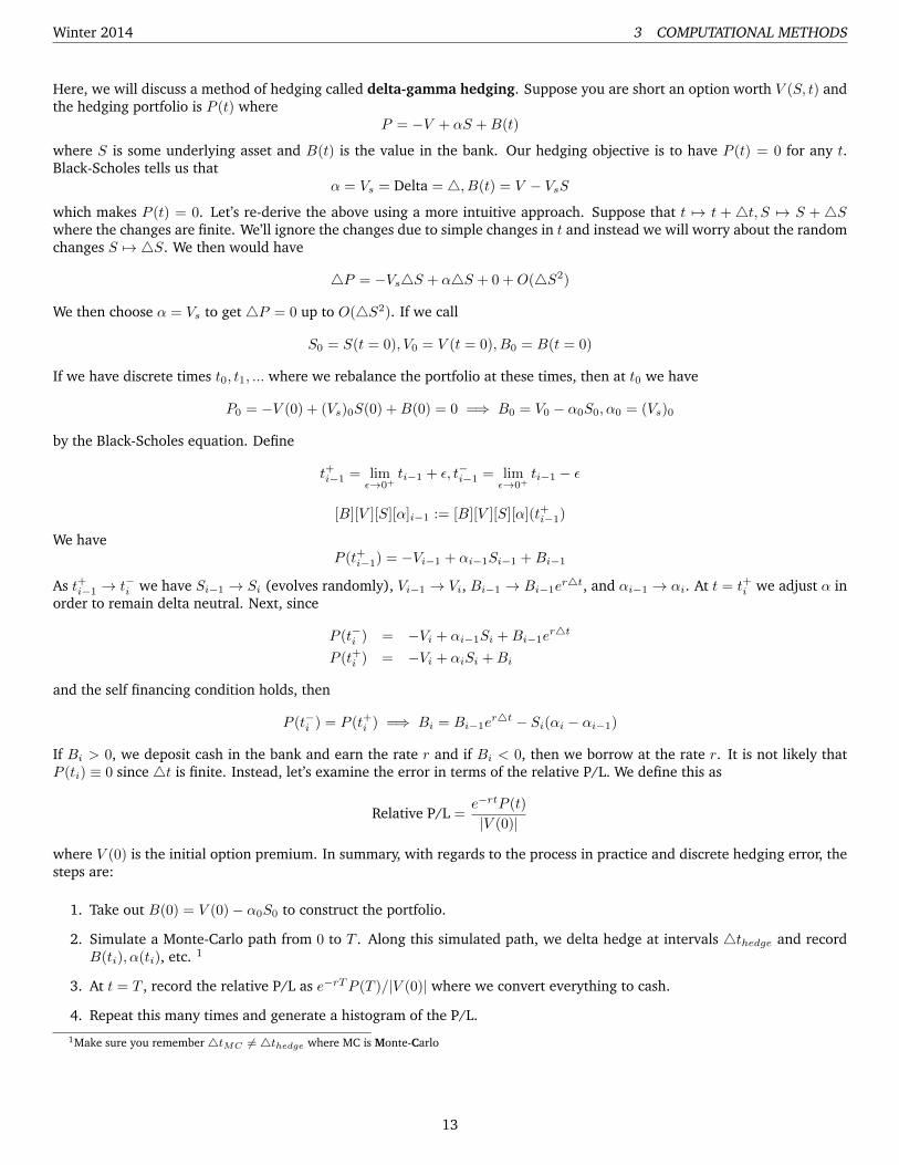
Here, we will discuss a method of hedging called delta-gamma hedging. Suppose you are short an option worth V (S, t) andthe hedging portfolio is P (t) where

P = −V + αS +B(t)

where S is some underlying asset and B(t) is the value in the bank. Our hedging objective is to have P (t) = 0 for any t.Black-Scholes tells us that

α = Vs = Delta = 4, B(t) = V − VsS

which makes P (t) = 0. Let’s re-derive the above using a more intuitive approach. Suppose that t 7→ t +4t, S 7→ S +4Swhere the changes are finite. We’ll ignore the changes due to simple changes in t and instead we will worry about the randomchanges S 7→ 4S. We then would have

4P = −Vs4S + α4S + 0 +O(4S2)

We then choose α = Vs to get 4P = 0 up to O(4S2). If we call

S0 = S(t = 0), V0 = V (t = 0), B0 = B(t = 0)

If we have discrete times t0, t1, ... where we rebalance the portfolio at these times, then at t0 we have

P0 = −V (0) + (Vs)0S(0) +B(0) = 0 =⇒ B0 = V0 − α0S0, α0 = (Vs)0

by the Black-Scholes equation. Define

t+i−1 = limε→0+

ti−1 + ε, t−i−1 = limε→0+

ti−1 − ε

[B][V ][S][α]i−1 := [B][V ][S][α](t+i−1)

We haveP (t+i−1) = −Vi−1 + αi−1Si−1 +Bi−1

As t+i−1 → t−i we have Si−1 → Si (evolves randomly), Vi−1 → Vi, Bi−1 → Bi−1er4t, and αi−1 → αi. At t = t+i we adjust α in

order to remain delta neutral. Next, since

P (t−i ) = −Vi + αi−1Si +Bi−1er4t

P (t+i ) = −Vi + αiSi +Bi

and the self financing condition holds, then

P (t−i ) = P (t+i ) =⇒ Bi = Bi−1er4t − Si(αi − αi−1)

If Bi > 0, we deposit cash in the bank and earn the rate r and if Bi < 0, then we borrow at the rate r. It is not likely thatP (ti) ≡ 0 since 4t is finite. Instead, let’s examine the error in terms of the relative P/L. We define this as

Relative P/L =e−rtP (t)

|V (0)|

where V (0) is the initial option premium. In summary, with regards to the process in practice and discrete hedging error, thesteps are:

1. Take out B(0) = V (0)− α0S0 to construct the portfolio.

2. Simulate a Monte-Carlo path from 0 to T . Along this simulated path, we delta hedge at intervals 4thedge and recordB(ti), α(ti), etc. 1

3. At t = T , record the relative P/L as e−rTP (T )/|V (0)| where we convert everything to cash.

4. Repeat this many times and generate a histogram of the P/L.

1Make sure you remember 4tMC 6= 4thedge where MC is Monte-Carlo

13


Note that if X is the P/L and p(X) is the probability density then p(x) dx is the probability of P/L in [x, x+ dx],

p(a) ∼ 1

b− a· # of occurences in [a, b]

total # of outcomes

Remark that under any hedging strategy, there would be more concentration in the density function around 0 P/L.

Delta-Gamma Hedging

Suppose we add an additional security to the hedging portfolio. Let the value of this security be I(s, t). The new portfolio is

P (t) = −V + αS + βI +B

where β is the number of units held in this security. As S 7→ S +4S,

P (t+4t, S +4S) = P (t, S) + Pt(t, S)4t+∂P

∂S4S +

∂2P

∂S2· (4S)2

2+ ...

and if we define 4P = P (t+4t, S +4S)− P (t, s), then

4P = Pt4t+ PS4S + PSS(4S)2

2+ ...

If we ignore the Pt term (assume it is deterministic) and set ∂P∂S = 0 and ∂2P∂S2 = 0. The former is called delta and the latter is

called gamma. Then, when we calculate these expressions explicitly:

∂P

∂S=

∂

∂S[−V + αS + βI +B(t)] = −Vs + α+ βIs + 0

∂2P

∂S2= −Vss + βIss

this implies that (1) −Vs+α+βIs = 0 and (2) −Vss+βIss = 0. We use the previous equations to calculate β at each rebalancepoint Note that β = Vss/Iss and we want I to have large gamma (|Iss| � 1). At time t = 0, P (0) = 0, B(0) = V0−α0S0−βI0.At the ith rebalance time,

(3) Bi = er4tBi−1 − Si(αi − αi−1)− Ii(βi − βi−1)

Delta-gamma hedging is defined by equations (1), (2), (3). This strategy thins the tails where the right tail is thicker thanthe left.

Delta-Vega Hedging

Suppose instead, we want to hedge against random changes in volatility. That is, we regard (S, σ) as random variables andset ∂P

∂S = 0 and ∂P∂σ = 0 where the latter is called vega and

∂P

∂σ= −Vσ + 0 + βIσ + 0 = 0 =⇒ β = Vσ/Iσ

3.7 Random Number Generation

Standard library algorithms generate pseudo-random numbers X ∼ U [0, 1] and until recently, library software for randomnumber generation was very bad. Imagine sampling a hypercube in d dimensions. The standard approach is to generatenumbers Xi for i = 1, ..., d where Xi ∼ U [0, 1].

For this random d dimensional vector X = [X1 · · ·Xd], the sample points would lie on hyperplanes in the cube!

The “Gold Standard” method for generating U [0, 1] is the Mersenne Twister which has many public codes available online.See the notes for reference [1998]. The properties of the twister are:

• It has period 219937 − 1

14


– That is, if we make 109 draws/second, the time to repeat a number� the age of the universe

• Probably good properties for d ≤ 623

• The Matlab default is the Twister

Assume we have a good method for generating U [0, 1] numbers. We want to generate Y ∼ N(0, 1). To do this, we use theconcept of a transformation of probabilities. To begin, suppose that p(x) dx is the probability of finding x ∈ [x, x + dx]. Itis obvious that

P (a ≤ x ≤ b) =

� b

a

p(x) dx,

� ∞−∞

p(x) dx = 1

In the case of a standard uniform random variable (r.v.), we have p(x) = χx∈[0,1]. Assume that X is a r.v. with density p(x)

and let Y = Y (X), assuming dYdX > 0. That is, it is a monotone increasing function. Suppose we can solve Y = Y (X) for X

given Y where X = X(Y ). Then,

(1) P (X(α) ≤ X ≤ X(β)) =

� X(β)

X(α)

p(x) dx

(2) P (α ≤ Y ≤ β) =

� β

α

p̂(y) dy

where (1) = (2), p̂ is the density of y, and

� β

α

p̂(y) dy =

� X(β)

X(α)

p(x) dx =

� β

α

[p(X(y))

dX

dy

]dy

As we let [α, β]→ 0 we get that p(X(y))dXdy = p̂(y). We repeat the argument for dYdX to the get the result that given a random

variable X with density p(x) and a monotone function y = y(x), then the density of y, p̂(y) is

p̂(y) = p(X(y))

∣∣∣∣dXdy∣∣∣∣

In our original problem, we have X ∼ U [0, 1] and we want to find Y (X) such that Y ∼ N(0, 1). That is, we want

p̂(Y ) =1√2πe−y

2/2, y ∈ (−∞,+∞)

Since p(x) = χx∈[0,1], then

χx∈[0,1]

∣∣∣∣dXdy∣∣∣∣ = χx∈[0,1]

dX

dy=e−y

2/2

√2π

=⇒ e−y2/2

√2π

dy = χx∈[0,1]dX

and integrating,

X =

� y

−∞

e−y2/2

√2π

dy + C

We can set the constant by noting that X → 0 =⇒ y → −∞ and X → 1 =⇒ y →∞. It can be shown that

X =

� y

−∞

e−y2/2

√2π

dy

This actually defines the transformation that we need and is the called the Fundamental Law of Transformation of Proba-bilities. So if we generate X ∼ U [0, 1] then to generate Y ∼ N(0, 1) we find y such that

X =

� y

−∞

e−y2/2

√2π

dy

or y = F−1(x) where F−1 is the inverse cumulative normal distribution function. While there is a built-in Matlab function,evaluating F−1 is very slow. To speed up computation, we use the Box-Muller method as follows.

15


Suppose we have a set of random points, (X1, X2) in 2D. Suppose the density is p(x1, x2). Suppose there exists functionsY1 = Y1(X1, X2) and Y2 = Y2(X1, X2). The 2D version of the Fundamental Theorem of Transformation of Probabilities is

(3) p̂(Y1, Y2) = p(X1, X2)|J |, J = det

[∂X1

∂Y1

∂X1

∂Y2∂X2

∂Y1

∂X2

∂Y2

]

Suppose that (X1, X2) ∼ (U [0, 1])2 with X1 ∼ U [0, 1], X2 ∼ U [0, 1], and p(X1, X2) = χ(X1,X2)∈[0,1]2 . So given this descriptionalong with Y1 = Y1(X1, X2), Y2 = Y2(X1, X2) then p̂(Y1, Y2) = |J | from (3). Consider

Y1 =√−2 logX1 cos(2πX2)

Y2 =√−2 logX1 sin(2πX2)

We then have the solutions for (X1, X2) being

X1 = exp

[−Y

21 + Y 2

2

2

]X2 =

1

2πarctan

[Y2

Y1

]and

(4) |J | = 1√2πe−Y

21 /2

1√2πe−Y

22 /2

If (X1, X2) ∼ U [0, 1]2 the using (4), we generate p̂(Y1, Y2) as a product of standard normals where Y1 ∼ N(0, 1), Y2 ∼ N(0, 1).So the general algorithm for the standard Box-Muller is:

1. Generate X1 ∼ U [0, 1], X2 ∼ U [0, 1]

2. Set ρ =√−2 logX1

3. Set Y1 = ρ cos(2πX2) and Y2 = ρ sin(2πX2)

We can make this even more efficient using the Polar Form Box-Muller where we generate a random draw in the (X1, X2)plane such that (X1, X2) ∼ D(0, 1) where D(0, 1) is the unit disk. To do this, we can try the following:

1. Create X1 ∼ U [0, 1], X2 ∼ U [0, 1], V1 = 2X1 − 1, V2 = 2X2 − 1, w = V 21 + V 2

2 , θ = tan(V2/V1)

2. If w < 1 then we accept

3. Otherwise go to Step 1

The probability of a successful draw is about π/4. It turns out that θ ∼ U [0, 2π], w ∼ U [0, 1]. Also note that

(5) cos θ = V1/√w

(6) sin θ = V2/√w

We can now create the modified algorithm as follows:

1. Generate X1 ∼ U [0, 1], X2 ∼ U [0, 1], V1 = 2X1 − 1, V2 = 2X2 − 1, w = V 21 + V 2

2 , θ = arctan(V2/V1)

2. Replace X1 by w ∼ U [0, 1] to set ρ =√−2 logw

3. Replace 2πX2 with θ to set Y1 = ρ cos(θ) and Y2 = ρ sin(θ)

4. Replace the trigonometric functions with the values above

The final form, implemented in actual algorithms, is:

1. Create X1 ∼ U [0, 1], X2 ∼ U [0, 1], V1 = 2X1 − 1, V2 = 2X2 − 1, w = V 21 + V 2

2 , θ = arctan(V2/V1)

2. If (w < 1), set Y1 = V1

√− 2 logw

w , Y2 = V2

√− 2 logw

w

3. Otherwise go to Step 1

16


3.8 Efficiency of Algorithms

A basic algorithm to compute the mean is to do the following:

Algorithm 1 Basic summationsum = 0

for i = 1,...,M

sum = sum + Xi

end

mean = sum / M

For single precision, the above algorithm is prone to floating point error accumulation. Older GPUs use single precision whilenewer ones can do double precision. To avoid loss of precision, do recursive pairwise summation.

Next, consider the basic integral approximation method in one dimension, under Monte Carlo, where

I1 =

� 1

0

f(x) dx ≈ 1

M

M∑i=1

f(Xi)

and Xi ∼ U [0, 1]. Using Monte Carlo, the work is O(M) and the error is O(1/√M). Alternatively, we can use the midpoint

rule of

I1 =

� 1

0

f(x) dx =

M∑i=1

f(Xi)4X +O(4X2)

where we have the same amount of complexity but the error is O(1/M2) = O(4X2). So the midpoint rule is more efficienterror-wise. Now imagine a d dimensional integral Id =

� 1

0

� 1

0...� 1

0f(~x)d~x. Under Monte Carlo we have,

Id =1

M

M∑i=1

f(~x) +O(1/√M)

and under the midpoint rule, where we fix the same work as Monte Carlo (fixed number of cells), we have

M =1

(4X)d

=⇒ 4X =1

M1/d

Id =

� 1

0

f(x) dx =

M∑i=1

f(Xi) (4X)d

+O(4X2)

Here, the work or complexity is the same as Monte Carlo (because we fixed it that way), but the error of the midpoint ruleis O(4X2) = O(1/M2/d). Note that this means that when the dimensionality is bigger than 4, then Monte Carlo beats themid-point rule error-wise.

Generalizing this to finance problems, consider the problem to pricing a high dimensional American Options. We have severalmethods in modern research today:

• Monte Carlo Backwards Stochastic Differential Equations (BSDEs)

• Sparse Grid Methods for PDEs

3.9 Correlated Random Numbers

Here we give some examples of options that depend on a basket of stock. The general form of an option on a basket of stocks{S1, S2, ..., Sd} has payoff

max [max{S1, S2, ..., Sd} −K, 0]

17


For example, a spread option with

dS1 = µ1S1dt+ σ1S1dZ

dS2 = µ2S2dt+ σ2S2dZ

with the correlation structure dZ1 · dZ2 = ρ12dt has the payoff

max [(S1 − S2)−K, 0]

Suppose we have observations of asset i, Si, at tk = k4t. The return of asset i in tk 7→ tk +4t is

Ri(tk) =Si(tk +4t)− Si(tk)

Si(tk)=⇒ R̄i =

M∑i=1

Ri(tk)

M

with historical volatility

σi =

√√√√ 1

4t(M − 1)

M∑k=1

(Ri(tk)− R̄2i )

and covariance

Cov(Ri, Rj) =1

4t(M − 1)

M∑k=1

(Ri(tk)− R̄i)(Rj(tk)− R̄j)

This gives us the correlation

Cor(Ri, Rj) = ρij =Cov(Ri, Rj)

σiσj, ρij ∈ [−1, 1]

Suppose we use Monte Carlo (MC) to price a d dimensional basket:

Sn+1i = Sni + Sni [r4t+ σiφ

ni

√4t]

In order to simulate correlated GBM, we need

φni ∼ N(0, 1), E[φni φnj ] = ρij

but algorithms seen so far only generate independent variables.

Problem 3.1. Given independent ε1 to εd with εi ∼ N(0, 1), we have E[εiεj ] = δij where δij is the Kronecker-Delta function.We would like to generate φ1 to φd with φi ∼ N(0, 1) and E[φiφj ] = ρij .

Solution. To solve this, assume that we are given a matrix of correlation coefficients ρ̂ with [ρ̂ij ] = ρij . Assume that ρ̂is symmetric positive definite (SPD). Symmetry is trivial while if we assume that it is not positive definite, then at leastone random variable is a linear combination of the others and we can remove it with ρ̂ being SPD. From this, we performCholesky factorization on ρ̂ to get the form ρ̂ = LLT where L is lower triangular, and

[ρ̂]ij = ρij =∑k

LikLTik

Let ~φ =[φ1 φ2 · · · φd

]T, ~ε =

[ε1 ε2 · · · εd

]Twhere φi =

∑Lijεj and ~φ = Lε. We then have

φiφk =∑j

∑k

LijLklεlεj

=∑j

∑l

LijεjεlLTkl

18

Winter 2014 4 PARTIAL DIFFERENTIAL EQUATIONS

and hence

E[φiφk] =∑j

∑l

LijE[εjεl]LTkl

=∑j

∑l

LijδjlLTkl

=∑l

LijLTkl = [LLT ]ik = ρik

Summary 3. Given independent ε1 to εd with εi ∼ N(0, 1), we have E[εiεj ] = δij .

(1) Cholesky factor ρ̂ = LLT

(2) Generate ε1 to εd

(3) ~φ = L~ε =⇒ φi ∼ N(0, 1), E[φiφk] = ρij

Remark 3.1. For d = 2, ρ̂ =

[1 ρ

ρ 1

]and L =

[1 0

ρ√

1− ρ2

].

3.10 Hedging Parameters

In MC, if we compute V (S + h, t) and V (S, t) and try to calculate

∆ = limh→0

V (S + h, t)− V (S, t)

h

then for really small h, this algorithm is very unstable. To improve this slightly, use common random numbers where wecompute V (S + h, t) and V (S, t) using MC but the same seed for each t.

A better trick is to first consider the Black-Scholes equation

Vτ =σ2S2

2VSS + rSVS − rV

Let ∆ = VS and differentiate the above with respect to (w.r.t.) S to get

(1) ∆τ =σ2S2

2∆SS + (r + σ2)S∆S

Recall that the expected value of the option V̂ solves the PDE

(2) V̂ =σ2S2

2V̂SS + µSV̂S − ρV̂

Comparing (1) and (2), they have the same form if ρ = 0 and µ = r + σ2. This implies that ∆ is the expected value of∆(S, T ). We then can compute the payoff VS(S, T ) and compute paths using

dS = (r + σ2)S dt+ σS dZ

and ∆(S = S0, s = 0) = E∆[Payoff]. Remark that for the Gamma Γ, the payoff is undefined.

4 Partial Differential Equations

Consider the PDE

(2) V̂ =σ2S2

2V̂SS + µSV̂S − rV̂ , τ = T − t, τ ∈ [0, T ]

19


Let’s solvethis on a finite domain 0 ≤ τ ≤ T and 0 ≤ S ≤ Smax. The approach is to discretize the PDE and seek the solutionat discrete “nodes”. Let

V (Si, τn) = (Vτ )ni =

[σ2S2

2V̂SS

]ni

+[µSV̂S

]ni−[rV̂]ni

4.1 Finite Difference Approximations

We then define, with notation and not literal indices,

∆Xi−1/2 := Xi −Xi−1,∆Xi+1/2 := Xi+1 −Xi

and using Taylor series

fi+1 = fi + (fx)i∆Xi+1/2 + (fxx)i(∆Xi+1/2)2

2+ ...

If we solve the above for (fx)i, then

(fx)i =

(fi+1 − fi∆Xi+1/2

)+O(∆Xi+1/2)

with a 1st order truncation error. The above is called a forward difference. Similarly,

(fx)i =

(fi − fi+1

∆Xi−1/2

)+O(∆Xi−1/2)

which we call a backward difference. Suppose that ∆Xi+1/2 = ∆Xi−1/2 = ∆X. Then,

fi+1 = fi + (fx)i∆X + (fxx)i∆X2

2+O(∆X3)

fi−1 = fi − (fx)i∆X + (fxx)i∆X2

2+O(∆X3)

If we subtract the second from the first, then

(fx)i =

(fi+1 − fi−1

2∆x

)+O(∆x2)

and we call this the centered difference. More generally, if ∆Xi+1/2 6= ∆Xi−1/2 then

(fx)i =fi+1 − fi−1

(∆Xi+1/2 + ∆Xi−1/2)− (fxx)i

2(∆Xi+1/2 + ∆Xi−1/2) +O(∆X2

i+1/2) +O(∆X2i−1/2)

Now remark [Note that the Taylor series (must be derived) for the below will most likely be on the final!]

(fxx)i =

(fi+1−fi∆Xi+1/2

)−(fi−fi−1

∆Xi−1/2

)(

∆Xi+1−∆Xi−1/2

2

) +O(∆Xi+1 −∆Xi−1/2) +O

((X2

i+1/2)

∆Xi+1 + ∆Xi−1/2

)+O

((X2

i−1/2)

∆Xi+1 + ∆Xi−1/2

)

In the special case of ∆Xi+1 = ∆Xi−1/2 = ∆X then

(fxx)i =fi+1 − 2fi + fi−1

(∆X)2+O(∆X2)

4.2 Discretization Methods for PDEs

Going back the the notation at the beginning of this section, recall that

V (Si, τn) = (Vτ )ni =

[σ2S2

2V̂SS

]ni

+[µSV̂S

]ni−[rV̂]ni

20


We call[σ2S2

2 V̂SS

]ni

the diffusion term,[µSV̂S

]ni

the drift term, and[rV̂]ni

the discounting term. We want to discretize

this equation using finite difference methods.

(THE FOLLOWING NOTES ARE COMPLEMENTARY TO THE PDE SLIDES)

Definition 4.1. Let φ be a smooth function. The truncation error (T.E.) of a discretization for the B-S equation Vτ = LV is

TE = {(φτ )ni − (Lφ)ni } − [φτ − Lφ]ni

Definition 4.2. Let ∆Smax = maxi(Si+1 − Si) and ∆τmax = τn+1 − τn. A discretization of the Black-Scholes equation isconsistent if the T.E.→ 0 as ∆Smax → 0 and ∆τmax → 0.

Example 4.1. Consider the heat equation uτ = uss. Discretize to get

un+1i − uni

∆τ=uni−1 − 2uni + uni+1

(∆S)2

Let φ(S, τ) be a smooth function. Then,φn+1i − φni

∆τ= (φτ )ni +O(∆τ)

and similarlyφni−1 − 2φni + φni+1

(∆S)2= (φss)

ni +O(∆S2)

We then have

TE =

[(φn+1i − φni

∆τ

)−(φni−1 − 2φni + φni+1

(∆S)2

)]ni

− [φτ − φss]ni

= O(∆τ) +O(∆S2)→ 0

as ∆S → 0 and ∆τ → 0.

Example 4.2. In the B-S equation, we previously derived (in the slides)

V n+1i = V ni (1− (αi + βi + r)∆τ) + V ni−1αi∆τ + V ni+1βi∆τ, αi ≥ 0, βi ≥ 0

Suppose we have a mesh for our stock prices for indices i = 0, ..., q and Sq = Smax. At S0, where i = 0, the B-S equationbecomes

Vτ = −rV

A discretization of this DE gives us

V n+10 − V n0

∆τ= −rV n0 =⇒ V n+1

0 = V n0 (1− r∆τ)

At S = Smax = Sq we have

V n+1q ≈

{Sq Call0 Put

At τ = 0, we have

V 0i =

{max(Si −K, 0) Callmax(K − Si, 0) Put

, i = 0, ..., q − 1

Recall that the TE is O(∆τ) +O(∆S2). We then use the following algorithm for the explicit T.E. method:

In the Implicit method,

(3) V n+1i = V ni − (αi + βi + r)∆τV n+1

i + V n+1i−1 αi∆τ + V n+1

i+1 βi∆τ

(4) V ni = [1 + (αi + βi + r)∆τ ]V n+1i − αi∆V n+1

i−1 − βi∆τVn+1i+1

21

Winter 2014 5 STABILITY

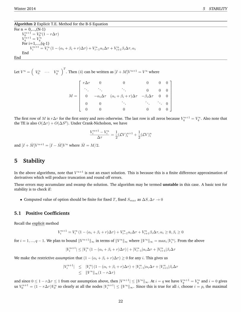
Algorithm 2 Explicit T.E. Method for the B-S EquationFor n = 0,...,(N-1)

V n+10 = V n0 (1− r∆τ)V n+1q = V nq

For i=1,...,(q-1)V n+1i = V ni (1− (αi + βi + r)∆τ) + V ni−1αi∆τ + V ni+1βi∆τ, αi

EndEnd

Let V n =(V n0 · · · V nq

)T. Then (4) can be written as [I +M ]V n+1 = V n where

M =

r∆τ 0 0 0 0 0. . .

. . .. . . 0 0 0

0 −αi∆τ (αi + βi + r)∆τ −βi∆τ 0 0

0 0. . .

. . .. . . 0

0 0 0 0 0 0

The first row of M is r∆τ for the first entry and zero otherwise. The last row is all zeros because V n+1

q = V nq . Also note thatthe TE is also O(∆τ) +O(∆S2). Under Crank-Nicholson, we have

V n+1i − V ni

∆τ=

1

2(LV )n+1

i +1

2(LV )ni

and [I + M̂ ]V n+1 = [I − M̂ ]V n where M̂ = M/2.

5 Stability

In the above algorithms, note that V n+1 is not an exact solution. This is because this is a finite difference approximation ofderivatives which will produce truncation and round off errors.

These errors may accumulate and swamp the solution. The algorithm may be termed unstable in this case. A basic test forstability is to check if:

• Computed value of option should be finite for fixed T , fixed Smax as ∆S,∆τ → 0

5.1 Positive Coefficients

Recall the explicit method

V n+1i = V ni (1− (αi + βi + r)∆τ) + V ni−1αi∆τ + V ni+1βi∆τ, αi ≥ 0, βi ≥ 0

for i = 1, ..., q − 1. We plan to bound ‖V n+1‖∞ in terms of ‖V n‖∞ where ‖V n‖∞ = maxi |V ni |. From the above

|V n+1i | ≤ |V ni (1− (αi + βi + r)∆τ) |+ |V ni−1|αi∆τ + |V ni+1|βi∆τ

We make the restrictive assumption that (1− (αi + βi + r)∆τ) ≥ 0 for any i. This gives us

|V n+1i | ≤ |V ni | (1− (αi + βi + r)∆τ) + |V ni−1|αi∆τ + |V ni+1|βi∆τ

≤ ‖V n‖∞(1− r∆τ)

and since 0 ≤ 1− r∆τ ≤ 1 from our assumption above, then |V n+1| ≤ ‖V n‖∞. At i = q we have V n+1q = V nq and i = 0 gives

us V n+10 = (1 − r∆τ)V n0 so clearly at all the nodes |V n+1

i | ≤ ‖V n‖∞. Since this is true for all i, choose i = p, the maximal

22


node, and get |V n+1p | = maxi |V n+1

i | = ‖V n+1‖∞ and

‖V n+1‖∞ ≤ ‖V n‖∞ =⇒ ‖V n+1‖∞ ≤ ‖V 0‖∞

We have thus derived sufficient conditions for stability:

αi, βi ≥ 0, [1− (αi + βi + r)∆τ ] ≥ 0

We can rearrange our assumption to get

∆τ ≤ mini

[1

(αi + βi + r)

]It turns out that this is a necessary and sufficient condition. Assume that ∆Si+1/2 = ∆Si−1/2 = ∆S and we are using centralweighting. The above equation becomes

∆τ ≤ mini

[1

σ2S2i

∆S2 + r

]≈[

∆S2

σ2S2i

]as ∆S → 0

Since Si = i∆S then ∆τ ≤ (1/(σ2q2)) where q ≡ # of nodes in the stock grid. This is pretty severe where the more nodesthat we have, the smaller our timesteps that we need for stability.

We now examine the stability of the fully implicit method. Recall that the equation for the implicit method was given as

V n+1i = V ni − (αi + βi + r)∆τV n+1

i + V n+1i−1 αi∆τ + V n+1

i+1 βi∆τ

for αi, βi ≥ 0. In cases,

V n+1i (1 + (αi + βi + r)∆τ) = V ni + V n+1

i−1 αi∆τ + V n+1i+1 βi∆τ

V n+10 = (1 + r∆τ)V n0

V n+1q = V nq

Using similar methods as before, we can show that

|V n+1i |(1 + (αi + βi + r)∆τ) ≤ ‖V ni ‖∞ + ‖V n+1

i−1 ‖∞αi∆τ + ‖V n+1i+1 ‖∞βi∆τ

Case 1: Suppose that p ∈ {1, ..., q − 1} and ‖V n+1‖∞ = |V n+1p |.

Then|V n+1i |(1 + (αi + βi + r)∆τ) ≤ ‖V n‖∞ + ‖V n+1‖∞αi∆τ + ‖V n+1‖∞βi∆τ

=⇒ ‖V n+1‖∞(1 + r∆τ) ≤ ‖V n‖∞=⇒ ‖V n+1‖∞ ≤ ‖V n‖∞

Hence, if ‖V n+1‖∞ = |V n+1p | for some p ∈ {1, ..., q − 1}, then ‖V n+1‖∞ ≤ ‖V n‖∞.

Case 2: Suppose that ‖V n+1‖∞ = |V n+10 |.

Then‖V n+1‖∞ ≤ ‖V n‖∞(1 + r∆τ)−1 ≤ ‖V n‖∞

Case 3: Suppose that ‖V n+1‖∞ = |V n+1q |.

Then trivially,‖V n+1‖∞ = ‖V n‖∞ =⇒ ‖V n+1‖∞ ≤ ‖V n‖∞

Hence ‖V n+1‖∞ ≤ ‖V n‖∞ for all n ∈ {1, ..., q} and the implicit method is stable. We also then have ‖V n+1‖∞ ≤ ‖V 0‖∞.Also, there are no conditions in the implicit method for it to be stable (so it is an efficient method).

Also remark that

V n+1i =

V ni + V n+1i−1 αi∆τ + V n+1

i+1 βi∆τ

1 + (αi + βi + r)∆τ

23


is a subconvex combination (sum of the top coefficients over the bottom is ≤ 1) and so we can infer (with a few more steps)or make intuition that that V n+1

i is smaller than V ni , Vn+1i−1 , or V n+1

i+1 .

The explicit also has this property as well:

V n+1i = V ni (1− (αi + βi + r)∆τ) + V ni−1αi∆τ + V ni+1βi∆τ

5.2 Crank-Nicholson Method

Recall that

M̂ =

r∆τ2 0 0 0 0 0

. . .. . .

. . . 0 0 0

0 −αi∆τ2

(αi+βi+r)∆τ2

−βi∆τ2 0 0

0 0. . .

. . .. . . 0

0 0 0 0 0 0

and the time stepping method was [I + M̂ ]V n+1 = [I − M̂ ]V n. Assume that M̂ has p linearly independent eigenvectors.Recall that ~x is an eigenvector of M̂ , then

M̂~v = λ~x, λ ∈ C

Let ~xi be the ith eigenvector with corresponding eigenvalue λi. We can write the time stepping method as V n+1 = [I +M̂ ]−1[I − M̂ ]V n and if V0 =

∑pi=1 ci~xi then

V n+1 =∑i

ci

[1− λi1 + λi

]n+1

~xi

In order for the above to be bounded, we must have ∣∣∣∣1− λi1 + λi

∣∣∣∣ ≤ 1

The above will hold when <(λi) ≥ 0 (will be shown below). We also note that M̂ has the properties

M̂ii ≥ 0

|M̂ii| ≥∑j 6=i

|M̂ij |

An improvement to Crank-Nicholson is the use of Rannacher smoothing. This involve two fully implicit timesteps beforeapply Crank-Nicholson.

Theorem 5.1. (Gershgorin Circle Theorem) Every eigenvalue of M̂ satisfies at least one of the inequalities∣∣∣M̂ii − λ∣∣∣ ≤∑

j 6=i

|M̂ij |

Corollary 5.1. Since |M̂ii| ≥∑j |M̂ij | then |M̂ii − λ| ≤ |M̂ii|. Therefore, all eigenvalues of M̂ has <(λi) ≥ 0.

So Crank-Nicholson (C-N) satisfies the necessary conditions for stability. In general, it is difficult to show that C-N satisfiessufficient conditions for stability. Here is the hand-wavy general approach. Suppose that

V n = BV n−1, B = [I +M ]−1[I −M ] =⇒ ‖V n‖‖V 0‖

≤ ‖Bn‖

We need to show thatlimP→Q

‖Bn‖ ≤ C

Where P → Q are the convergence conditions n→∞, ∆t→ 0, ∆S → 0, n∆t = t.

24

Winter 2014 6 LATTICE VS. FINITE DIFFERENCE METHODS

Simple Case

Suppose B is a normal matrix where BTB = BBT . If B is normal, then there is a unitary matrix Q which diagonalizes Bsuch that tr(Q−1BQ) =

∑i λi where Q−1BQ = Λ contains eigenvalues along the diagonal and 0 elsewhere.

Theorem 5.2. If B is normal, the if maxi |λi| = |λmax| ≤ 1 as ∆S → 0, then

limn→∞,∆S→0

‖Bn+1‖2 ≤ C0, C0 ∈ R

Proof. We know that B = QΛQ−1 and so

Bn = (QΛQ−1)(QΛQ−1)... = QΛnQ−1

=⇒ ‖Bn‖2 ≤ ‖Q‖2‖Q−1‖2‖Λn‖2

=⇒ ‖Bn‖2 ≤ |λmax|n ≤ 1

General Case

In the general case, we can put B into the Jordan normal form B = U−1JU where J is a matrix of diagonal blocks ofgeneralized eigenvalues with ones on the above off diagonal. Since U is not unitary, in general, ‖U−1‖2‖U‖2 may not bebounded as ∆S → 0. It also may not be possible to bound Jn.

In general, it is possible to show that C-N is unconditionally stable, but it’s not easy. Lax-Wendroff Theorem makes someheadway into this proof.

5.3 Von-Neumann Analysis

Other techniques for stability are:

• Von-Neumann Analysis

– See notes

– Only works for constant coefficients

6 Lattice vs. Finite Difference Methods

A lattice method is an explicit finite difference method and uses a special grid. Recall that VFD = VExact + (∆τ,∆S2). Wewill show that

|VLattice − VFD| = O(∆τ)

Now recall the properties of a lattice method:

• Discrete random walk on a lattice

• Parameters selected so that the walk converges to

dS

S= µdt+ σdZ

25


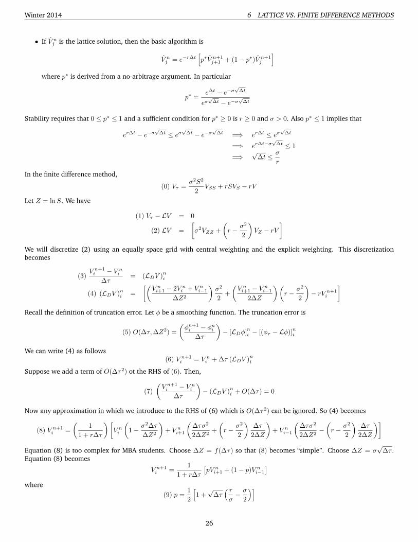
• If V̂ nj is the lattice solution, then the basic algorithm is

V̂ nj = e−r∆t[p∗V̂ n+1

j+1 + (1− p∗)V̂ n+1j

]where p∗ is derived from a no-arbitrage argument. In particular

p∗ =e∆t − e−σ

√∆t

eσ√

∆t − e−σ√

∆t

Stability requires that 0 ≤ p∗ ≤ 1 and a sufficient condition for p∗ ≥ 0 is r ≥ 0 and σ > 0. Also p∗ ≤ 1 implies that

er∆t − e−σ√

∆t ≤ eσ√

∆t − e−σ√

∆t =⇒ er∆t ≤ eσ√

∆t

=⇒ er∆t−σ√

∆t ≤ 1

=⇒√

∆t ≤ σ

r

In the finite difference method,

(0) Vτ =σ2S2

2VSS + rSVS − rV

Let Z = lnS. We have

(1) Vτ − LV = 0

(2) LV =

[σ2VZZ +

(r − σ2

2

)VZ − rV

]We will discretize (2) using an equally space grid with central weighting and the explicit weighting. This discretizationbecomes

(3)V n+1i − V ni

∆τ= (LDV )

ni

(4) (LDV )ni =

[(V ni+1 − 2V ni + V ni−1

∆Z2

)σ2

2+

(V ni+1 − V ni−1

2∆Z

)(r − σ2

2

)− rV n+1

i

]Recall the definition of truncation error. Let φ be a smoothing function. The truncation error is

(5) O(∆τ,∆Z2) =

(φn+1i − φni

∆τ

)− [LDφ]

ni − [(φτ − Lφ)]

ni

We can write (4) as follows(6) V n+1

i = V ni + ∆τ (LDV )ni

Suppose we add a term of O(∆τ2) ot the RHS of (6). Then,

(7)

(V n+1i − V ni

∆τ

)− (LDV )

ni +O(∆τ) = 0

Now any approximation in which we introduce to the RHS of (6) which is O(∆τ2) can be ignored. So (4) becomes

(8) V n+1i =

(1

1 + r∆τ

)[V ni

(1− σ2∆τ

∆Z2

)+ V ni+1

(∆τσ2

2∆Z2+

(r − σ2

2

)∆τ

2∆Z

)+ V ni−1

(∆τσ2

2∆Z2−(r − σ2

2

)∆τ

2∆Z

)]Equation (8) is too complex for MBA students. Choose ∆Z = f(∆τ) so that (8) becomes “simple”. Choose ∆Z = σ

√∆τ .

Equation (8) becomes

V n+1i =

1

1 + r∆τ

[pV ni+1 + (1− p)V ni−1

]where

(9) p =1

2

[1 +√

∆τ( rσ− σ

2

)]

26


Now(10) e−r∆τ =

1

1 + r∆τ+O(∆τ2)

Combining (9) and (10) gives usV n+1i = e−r∆τ

(pV ni+1 + (1− p)V ni−1

)+O(∆τ2)

For stability, we must have 0 ≤ p ≤ 1 which is to say

(11) − 1 ≤√

∆τ( rσ− σ

2

)≤ 1

The final FD expression then becomes

(12) V n+1i = e−r∆τ

(pV ni+1 + (1− p)V ni−1

)From here, we have something which we will refer to as the domain problem:

• The PDE domain is [Smin, Smax] and [lnSmin, lnSmax]

• In the lattice domain, as ∆τ → 0 we have maxj V̂Nj →∞ and minj V̂

Nj →∞

• To make the lattice method become closer to the PDE method, we bound the Sj values above and below by Smax

and Smin respectively and apply the PDE boundary conditions on the Smin and Smax nodes. This is called creating anon-exploding tree.

We then swap some indices by taking ∆t as ∆τ and switching n and n+ 1 to get

(12) V ni = e−r∆t(pV n+1

i+1 + (1− p)V n+1i−1

)Now let Zi = lnSi, ∆Z = Zi+1 − Zi = ln(Si+1/Si) which gives us

Si+1 = Sie∆Z = Sie

σ√

∆t

Si−1 = Sie−∆Z = Sie

−σ√

∆t

If Si(FD) = Snj (Lattice) then

Si+1 = Sieσ√

∆t = Snj eσ√

∆t = Sn+1j+1

Si−1 = Sie−σ√

∆t = Snj e−σ√

∆t = Sn+1j

In summary,

FD Index Lattice Index

V ni V njV n+1i+1 V n+1

j+1

V n+1i−1 V n+1

j

If we replace the FD indices with lattice indices, then

(16) V ni = e−r∆t(pV n+1

j+1 + (1− p)V n+1j

)where the lattice expression is

V̂ ni = e−r∆t(p∗V n+1

i+1 + (1− p∗)V n+1i−1

)Now

(17) p∗ =e∆t − e−σ

√∆t

eσ√

∆t − e−σ√

∆t

(18) p =1

2

[1 +√

∆τ( rσ− σ

2

)]27


You can show, after some tedious algebra,

(19) p∗ = p+ c1(∆t)3/2 +O(∆t2)

If we put (19) into (17), we get

(20) V̂ ni = e−r∆t[pV n+1

i+1 + (1− p)V n+1i−1

]+ e−r∆t

[c1(∆t)3/2

(V̂ n+1j+1 − V̂

n+1j

)]+O(∆t2)

Assume that V̂ (Snj , tn) has bounded derivatives:

V̂ n+1j+1 − V̂

n+1j

∆Z=

(∂V

∂Z

)n+1

j+ 12

+O(∆Z2)

=⇒ (21) (V̂ n+1j+1 − V̂

n+1j ) = (VZ)n+1

j+ 12

(∆Z) +O(∆Z3)

= O(∆Z) = O(√

∆t)

Putting (21) into (20) gives(22) V̂ nj = e−r∆t

[pV̂ n+1

j+1 + (1− p)V n+1j

]+O(∆t)

The finite difference equation is(23) V nj = e−r∆t

[pV̂ n+1

j+1 + (1− p)V n+1j

]Let Enj = (V nj − V̂ nj ) and subtract (22) from (23) to get

(24) Enj = e−r∆t[pEn+1

j+1 + (1− p)En+1j

]+O(∆t2)

Choose ∆t sufficiently small so that 0 ≤ p ≤ 1. By the triangle inequality,

(24A) |Enj | ≤ p|En+1j+1 |+ (1− p)|En+1

j |+ c2∆t2

where c2 is some constant independent of ∆t. Let (25) ‖En‖∞ = maxj |Enj |. Using (25) in (24A) gives us

(26) ‖En‖∞ ≤ ‖En+1‖∞ + c2∆t2

Recursion gives us

‖E0‖∞ ≤ ‖E1‖∞ + c2∆t ≤ ... ≤ ‖EN‖∞︸︷︷︸=0

+T

∆tc2(∆t)2 = O(∆t)

The final result is that |V̂ 00 − V 0

0 | = O(∆t). Hence the lattice methods is simply a special case of an explicit finite differencemethod.

Summary 4. Recall that:

• Lattice Method

– Equally spaced grid in Z = lnS space

– Choice of timestep ensures method is stable and positive coefficient

– We have specified the grid spacing without regard to the contract

∗ For example, consider the barrier option. The barrier knock-out condition is

V (S, ti) = 0 ifS ≥ β

where ti is the observation time. Let t−i = ti − ε, 0 < ε� 1, τ = T − t, τ+i = T − t−i where

V (S, t−i ) = 0 if S ≥ β ⇐⇒ V (S, t+i ) = 0 if S ≥ β

28


Consider a simple example with two observations t = t1, T and 0 < t1 < T . With a barrier of β and a strike ofK, a knock-out call has payoff

V (S, T ) =

0 S ∈ [0,K)

S −K S ∈ [K,B)

0 S ∈ [B,∞)

Moving the PDE from τ = 0 to τ−1 creates a smoothed curve V (S, τ−1 ) ≥ V (S, T ) where it increases concaveup from 0 to B and decreases sharply (but continuously) from B onwards. Moving from τ−1 to τ+

1 is almostthe same as V (S, τ−1 ) but there is a jump down at B to 0 (jump discontinuity). As τ+

1 goes to T , the wholecurve smooths over and it is continuous again. In a lattice grid, we don’t have a choice to place nodes near Kor B.

Summary 5. (Final Exam)

• 1 to 4 are trivial questions

• 5 to 6 are related to assignment or practice problems

• 7 is the most difficult question

29

Winter 2014 INDEX

Indexarbitrage, 1

backward difference, 20bid-ask spread, 2boundary conditions, 7Box-Muller method, 15Brownian motion with drift, 3

centered difference, 20Cholesky factorization, 18CIR Model, 12Crank-Nicholson Method, 24

delta, 8, 14delta-gamma hedging, 13diffusion term, 21discounting term, 21domain problem, 27drift term, 21

European call, 1European put, 1explicit finite difference method, 25

forward difference, 20fully implicit method, 23Fundamental Law of Transformation of Probabilities, 15

gamma, 14Gershgorin Circle Theorem, 24

HJB PDE, 7

infinitely jagged, 4integral, 17Ito definition, 5Ito integral, 5

Kronecker-Delta function, 18

lattice grid, 29lattice method, 25lattice model, 3Lax-Wendroff Theorem, 25

Markov process, 3mean, 17Mersenne Twister, 14midpoint rule, 17

no-arbitrage price, 10non-exploding tree, 27

optimal stochastic control, 7

Polar Form Box-Muller, 16

Rannacher smoothing, 24real probability, 8real-expected value, 10risk-free rate, 2risk-neutral probability, 8risk-neutral world, 10

self-financing, 7short position, 2Stratonovich definition, 5subadditive property, 12symmetric positive definite, 18

tail risk, 12transformation of probabilities, 15truncation error, 21

unstable, 22

value-at-risk, 12vega, 14Von-Neumann Analysis, 25

weak error, 10

30

Documents

CS 476 (Winter 2014 - 1141) - GitHub Pages