CS 412 Intro. to Data Mining - University Of Illinoisweb.engr.illinois.edu/~hanj/cs412/bk3_slides/06FPBasic.pdf · CS 412 Intro. to Data Mining Chapter 6. ... Ex. sup{Beer, Eggs}

$Page 1: CS 412 Intro. to Data Mining - University Of Illinoisweb.engr.illinois.edu/~hanj/cs412/bk3_slides/06FPBasic.pdf · CS 412 Intro. to Data Mining Chapter 6. ... Ex. sup{Beer, Eggs}$
CS 412 Intro. to Data MiningChapter 6. Mining Frequent Patterns, Association

and Correlations: Basic Concepts and MethodsJiawei Han, Computer Science, Univ. I llinois at Urbana -Champaign, 2017

1

2

3

Chapter 6: Mining Frequent Patterns, Association and Correlations: Basic Concepts and Methods

Basic Concepts

Efficient Pattern Mining Methods

Pattern Evaluation

Summary

4

Pattern Discovery: Basic Concepts

What Is Pattern Discovery? Why Is It Important?

Basic Concepts: Frequent Patterns and Association Rules

Compressed Representation: Closed Patterns and Max-Patterns

5

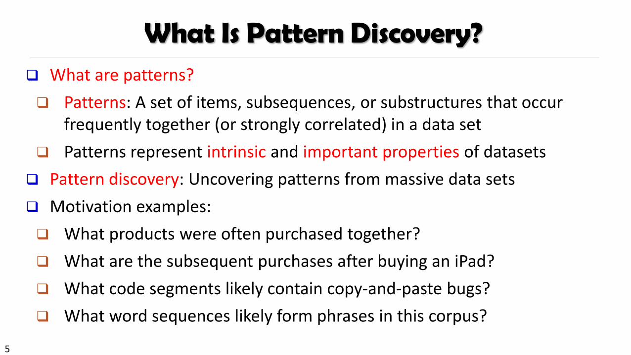
What Is Pattern Discovery? What are patterns?

Patterns: A set of items, subsequences, or substructures that occur frequently together (or strongly correlated) in a data set

Patterns represent intrinsic and important properties of datasets

Pattern discovery: Uncovering patterns from massive data sets

Motivation examples:

What products were often purchased together?

What are the subsequent purchases after buying an iPad?

What code segments likely contain copy-and-paste bugs?

What word sequences likely form phrases in this corpus?

6

Pattern Discovery: Why Is It Important? Finding inherent regularities in a data set

Foundation for many essential data mining tasks

Association, correlation, and causality analysis

Mining sequential, structural (e.g., sub-graph) patterns

Pattern analysis in spatiotemporal, multimedia, time-series, and stream data

Classification: Discriminative pattern-based analysis

Cluster analysis: Pattern-based subspace clustering

Broad applications

Market basket analysis, cross-marketing, catalog design, sale campaign analysis, Web log analysis, biological sequence analysis

7

Basic Concepts: k-Itemsets and Their Supports Itemset: A set of one or more items

k-itemset: X = {x1, …, xk}

Ex. {Beer, Nuts, Diaper} is a 3-itemset

(absolute) support (count) of X, sup{X}: Frequency or the number of occurrences of an itemset X

Ex. sup{Beer} = 3

Ex. sup{Diaper} = 4

Ex. sup{Beer, Diaper} = 3

Ex. sup{Beer, Eggs} = 1

Tid Items bought

10 Beer, Nuts, Diaper

20 Beer, Coffee, Diaper

30 Beer, Diaper, Eggs

40 Nuts, Eggs, Milk

50 Nuts, Coffee, Diaper, Eggs, Milk

(relative) support, s{X}: The fraction of transactions that contains X (i.e., the probability that a transaction contains X)

Ex. s{Beer} = 3/5 = 60%

Ex. s{Diaper} = 4/5 = 80%

Ex. s{Beer, Eggs} = 1/5 = 20%

8

Basic Concepts: Frequent Itemsets (Patterns) An itemset (or a pattern) X is frequent

if the support of X is no less than a minsup threshold σ

Let σ = 50% (σ: minsup threshold)

For the given 5-transaction dataset

All the frequent 1-itemsets:

Beer: 3/5 (60%); Nuts: 3/5 (60%)

Diaper: 4/5 (80%); Eggs: 3/5 (60%)

All the frequent 2-itemsets:

{Beer, Diaper}: 3/5 (60%)

All the frequent 3-itemsets?

None

Tid Items bought




40 Nuts, Eggs, Milk


Why do these itemsets (shown on the left) form the complete set of frequent k-itemsets (patterns) for any k?

Observation: We may need an efficient method to mine a complete set of frequent patterns

9

From Frequent Itemsets to Association Rules Comparing with itemsets, rules can be more telling

Ex. Diaper Beer

Buying diapers may likely lead to buying beers

How strong is this rule? (support, confidence)

Measuring association rules: X Y (s, c)

Both X and Y are itemsets

Support, s: The probability that a transaction contains X Y

Ex. s{Diaper, Beer} = 3/5 = 0.6 (i.e., 60%)

Confidence, c: The conditional probability that a transaction containing X also contains Y

Calculation: c = sup(X Y) / sup(X)

Ex. c = sup{Diaper, Beer}/sup{Diaper} = ¾ = 0.75

Note: X Y: the union of two itemsets The set contains both X and Y

Tid Items bought




40 Nuts, Eggs, Milk


Containing

diaper

Containing both

Containing beer

Beer Diaper{Beer} {Diaper}

{Beer} {Diaper} = {Beer, Diaper}

10

Mining Frequent Itemsets and Association Rules

Association rule mining

Given two thresholds: minsup, minconf

Find all of the rules, X Y (s, c)

such that, s ≥ minsup and c ≥ minconf

Tid Items bought




40 Nuts, Eggs, Milk

50 Nuts, Coffee, Diaper, Eggs, Milk Let minsup = 50%

Freq. 1-itemsets: Beer: 3, Nuts: 3, Diaper: 4, Eggs: 3

Freq. 2-itemsets: {Beer, Diaper}: 3

Let minconf = 50%

Beer Diaper (60%, 100%)

Diaper Beer (60%, 75%)

Observations:

Mining association rules and mining frequent patterns are very close problems

Scalable methods are needed for mining large datasets

(Q: Are these all rules?)

11

Challenge: There Are Too Many Frequent Patterns! A long pattern contains a combinatorial number of sub-patterns

How many frequent itemsets does the following TDB1 contain?

TDB1: T1: {a1, …, a50}; T2: {a1, …, a100}

Assuming (absolute) minsup = 1

Let’s have a try

1-itemsets: {a1}: 2, {a2}: 2, …, {a50}: 2, {a51}: 1, …, {a100}: 1,

2-itemsets: {a1, a2}: 2, …, {a1, a50}: 2, {a1, a51}: 1 …, …, {a99, a100}: 1,

…, …, …, …

99-itemsets: {a1, a2, …, a99}: 1, …, {a2, a3, …, a100}: 1

100-itemset: {a1, a2, …, a100}: 1

The total number of frequent itemsets:

A too huge set for any one to compute or store!

12

Expressing Patterns in Compressed Form: Closed Patterns

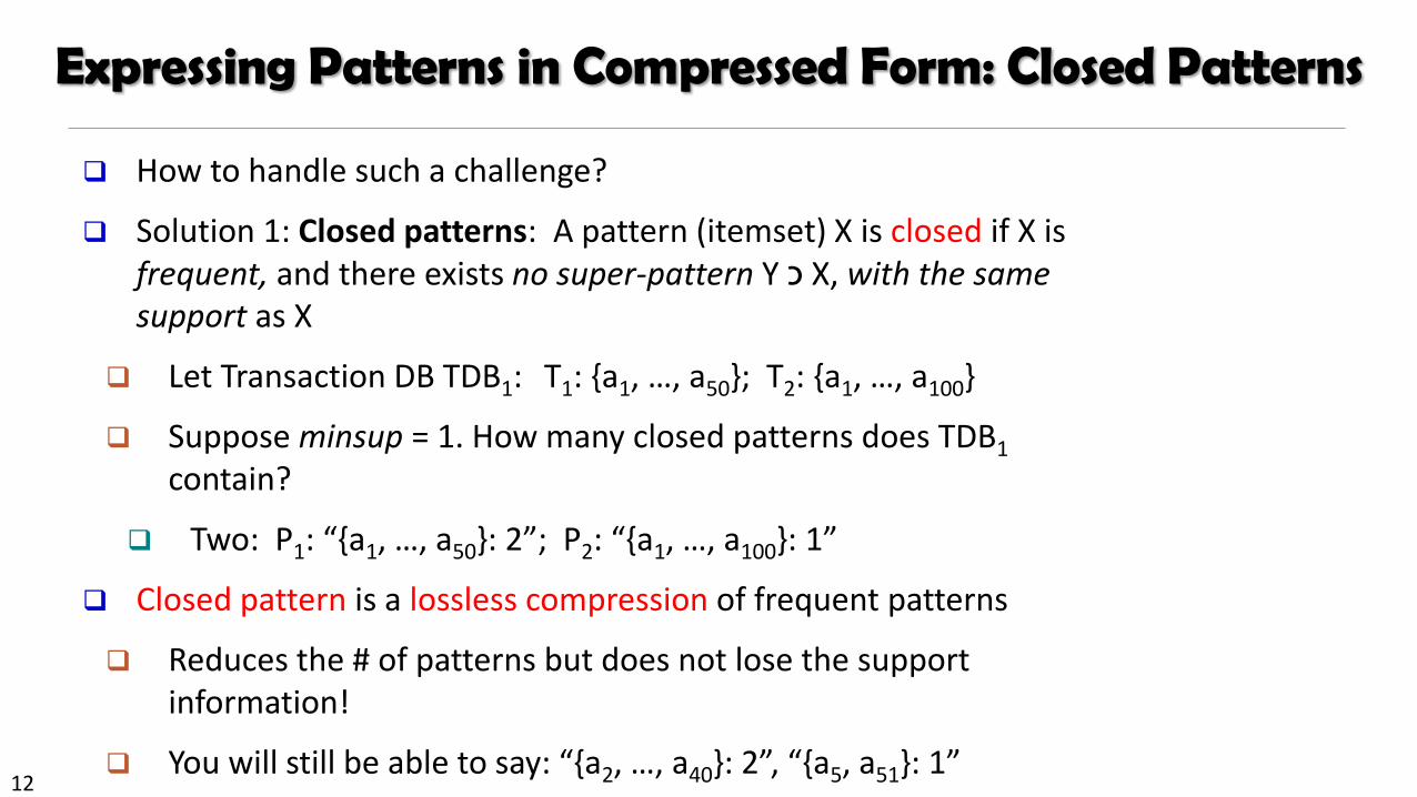
How to handle such a challenge?

Solution 1: Closed patterns: A pattern (itemset) X is closed if X is frequent, and there exists no super-pattern Y כ X, with the same support as X

Let Transaction DB TDB1: T1: {a1, …, a50}; T2: {a1, …, a100}

Suppose minsup = 1. How many closed patterns does TDB1

contain?

Two: P1: “{a1, …, a50}: 2”; P2: “{a1, …, a100}: 1”

Closed pattern is a lossless compression of frequent patterns

Reduces the # of patterns but does not lose the support information!

You will still be able to say: “{a2, …, a40}: 2”, “{a5, a51}: 1”

13

Expressing Patterns in Compressed Form: Max-Patterns

Solution 2: Max-patterns: A pattern X is a max-pattern if X is

frequent and there exists no frequent super-pattern Y כ X

Difference from close-patterns?

Do not care the real support of the sub-patterns of a max-pattern

Let Transaction DB TDB1: T1: {a1, …, a50}; T2: {a1, …, a100}

Suppose minsup = 1. How many max-patterns does TDB1 contain?

One: P: “{a1, …, a100}: 1”

Max-pattern is a lossy compression!

We only know {a1, …, a40} is frequent

But we do not know the real support of {a1, …, a40}, …, any more!

Thus in many applications, mining close-patterns is more desirable than mining max-patterns

14


Basic Concepts


Pattern Evaluation

Summary

15


The Downward Closure Property of Frequent Patterns

The Apriori Algorithm

Extensions or Improvements of Apriori

Mining Frequent Patterns by Exploring Vertical Data Format

FPGrowth: A Frequent Pattern-Growth Approach

Mining Closed Patterns

16


Observation: From TDB1: T1: {a1, …, a50}; T2: {a1, …, a100}

We get a frequent itemset: {a1, …, a50}

Also, its subsets are all frequent: {a1}, {a2}, …, {a50}, {a1, a2}, …, {a1, …, a49}, …

There must be some hidden relationships among frequent patterns!

The downward closure (also called “Apriori”) property of frequent patterns

If {beer, diaper, nuts} is frequent, so is {beer, diaper}

Every transaction containing {beer, diaper, nuts} also contains {beer, diaper}

Apriori: Any subset of a frequent itemset must be frequent

Efficient mining methodology

If any subset of an itemset S is infrequent, then there is no chance for S to be frequent—why do we even have to consider S!? A sharp knife for pruning!

17

Apriori Pruning and Scalable Mining Methods

Apriori pruning principle: If there is any itemset which is

infrequent, its superset should not even be generated! (Agrawal &

Srikant @VLDB’94, Mannila, et al. @ KDD’ 94)

Scalable mining Methods: Three major approaches

Level-wise, join-based approach: Apriori (Agrawal & Srikant@VLDB’94)

Vertical data format approach: Eclat (Zaki, Parthasarathy, Ogihara, Li @KDD’97)

Frequent pattern projection and growth: FPgrowth (Han, Pei, Yin @SIGMOD’00)

18

Apriori: A Candidate Generation & Test Approach

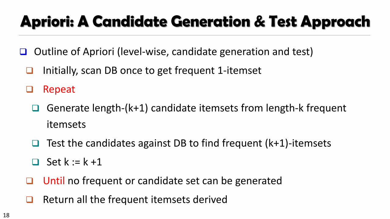
Outline of Apriori (level-wise, candidate generation and test)

Initially, scan DB once to get frequent 1-itemset

Repeat

Generate length-(k+1) candidate itemsets from length-k frequent

itemsets

Test the candidates against DB to find frequent (k+1)-itemsets

Set k := k +1

Until no frequent or candidate set can be generated

Return all the frequent itemsets derived

19

The Apriori Algorithm (Pseudo-Code)

Ck: Candidate itemset of size k

Fk : Frequent itemset of size k

K := 1;

Fk := {frequent items}; // frequent 1-itemset

While (Fk != ) do { // when Fk is non-empty

Ck+1 := candidates generated from Fk; // candidate generation

Derive Fk+1 by counting candidates in Ck+1 with respect to TDB at minsup;

k := k + 1

}

return k Fk // return Fk generated at each level

20

The Apriori Algorithm—An Example

Database TDB

1st scan

C1

F1

F2

C2 C2

2nd scan

C3 F33rd scan

Tid Items

10 A, C, D

20 B, C, E

30 A, B, C, E

40 B, E

Itemset sup

{A} 2

{B} 3

{C} 3

{D} 1

{E} 3

Itemset sup

{A} 2

{B} 3

{C} 3

{E} 3

Itemset

{A, B}

{A, C}

{A, E}

{B, C}

{B, E}

{C, E}

Itemset sup

{A, B} 1

{A, C} 2

{A, E} 1

{B, C} 2

{B, E} 3

{C, E} 2

Itemset sup

{A, C} 2

{B, C} 2

{B, E} 3

{C, E} 2

Itemset

{B, C, E}

Itemset sup

{B, C, E} 2

minsup = 2

21

abc abd acd ace bcd

abcd acde

self-join self-join

pruned

Apriori: Implementation Tricks How to generate candidates?

Step 1: self-joining Fk

Step 2: pruning

Example of candidate-generation

F3 = {abc, abd, acd, ace, bcd}

Self-joining: F3*F3

abcd from abc and abd

acde from acd and ace

Pruning:

acde is removed because ade is not in F3

C4 = {abcd}

22

Candidate Generation: An SQL Implementation

Suppose the items in Fk-1 are listed

in an order

Step 1: self-joining Fk-1

insert into Ck

select p.item1, p.item2, …, p.itemk-1, q.itemk-1

from Fk-1 as p, Fk-1 as q

where p.item1= q.item1, …, p.itemk-2 = q.itemk-2, p.itemk-1 < q.itemk-1

Step 2: pruning

for all itemsets c in Ck do

for all (k-1)-subsets s of c do

if (s is not in Fk-1) then delete c from Ck

abc abd acd ace bcd

abcd acde

self-join self-join

pruned

23

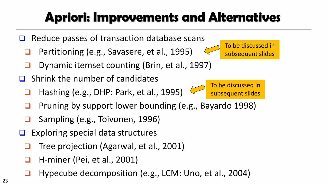
Apriori: Improvements and Alternatives

Reduce passes of transaction database scans

Partitioning (e.g., Savasere, et al., 1995)

Dynamic itemset counting (Brin, et al., 1997)

Shrink the number of candidates

Hashing (e.g., DHP: Park, et al., 1995)

Pruning by support lower bounding (e.g., Bayardo 1998)

Sampling (e.g., Toivonen, 1996)

Exploring special data structures

Tree projection (Agarwal, et al., 2001)

H-miner (Pei, et al., 2001)

Hypecube decomposition (e.g., LCM: Uno, et al., 2004)

To be discussed in subsequent slides

To be discussed in subsequent slides

24

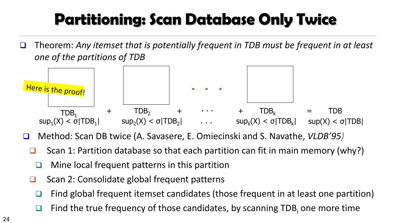
Partitioning: Scan Database Only Twice

Theorem: Any itemset that is potentially frequent in TDB must be frequent in at least one of the partitions of TDB

TDB1TDB2 TDBk+ = TDB++

sup1(X) < σ|TDB1| sup2(X) < σ|TDB2| supk(X) < σ|TDBk| sup(X) < σ|TDB|

. . .. . .

Method: Scan DB twice (A. Savasere, E. Omiecinski and S. Navathe, VLDB’95)

Scan 1: Partition database so that each partition can fit in main memory (why?)

Mine local frequent patterns in this partition

Scan 2: Consolidate global frequent patterns

Find global frequent itemset candidates (those frequent in at least one partition)

Find the true frequency of those candidates, by scanning TDBi one more time

25

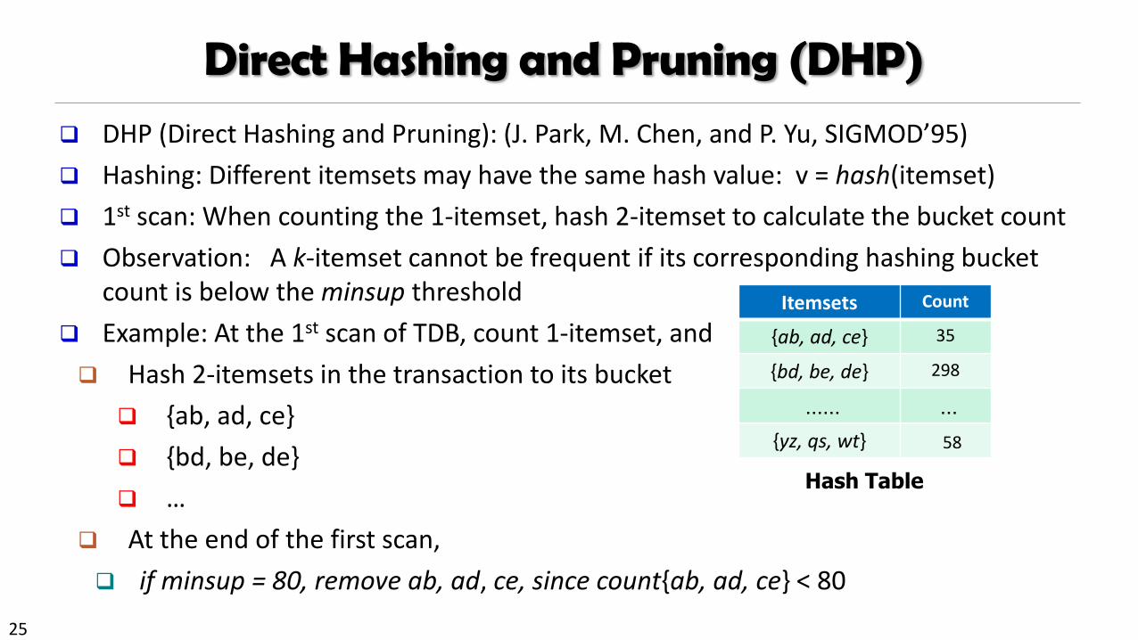
Direct Hashing and Pruning (DHP)

DHP (Direct Hashing and Pruning): (J. Park, M. Chen, and P. Yu, SIGMOD’95)

Hashing: Different itemsets may have the same hash value: v = hash(itemset)

1st scan: When counting the 1-itemset, hash 2-itemset to calculate the bucket count

Observation: A k-itemset cannot be frequent if its corresponding hashing bucket count is below the minsup threshold

Example: At the 1st scan of TDB, count 1-itemset, and

Hash 2-itemsets in the transaction to its bucket

{ab, ad, ce}

{bd, be, de}

…

At the end of the first scan,

if minsup = 80, remove ab, ad, ce, since count{ab, ad, ce} < 80

Hash Table

Itemsets Count

{ab, ad, ce} 35

{bd, be, de} 298

…… …

{yz, qs, wt} 58

26

Exploring Vertical Data Format: ECLAT ECLAT (Equivalence Class Transformation): A depth-first search

algorithm using set intersection [Zaki et al. @KDD’97]

Tid-List: List of transaction-ids containing an itemset

Vertical format: t(e) = {T10, T20, T30}; t(a) = {T10, T20}; t(ae) = {T10, T20}

Properties of Tid-Lists

t(X) = t(Y): X and Y always happen together (e.g., t(ac} = t(d})

t(X) t(Y): transaction having X always has Y (e.g., t(ac) t(ce))

Deriving frequent patterns based on vertical intersections

Using diffset to accelerate mining

Only keep track of differences of tids

t(e) = {T10, T20, T30}, t(ce) = {T10, T30} → Diffset (ce, e) = {T20}

A transaction DB in Horizontal Data Format

Item TidList

a 10, 20

b 20, 30

c 10, 30

d 10

e 10, 20, 30

The transaction DB in Vertical Data Format

Tid Itemset

10 a, c, d, e

20 a, b, e

30 b, c, e

27

Why Mining Frequent Patterns by Pattern Growth?

Apriori: A breadth-first search mining algorithm

First find the complete set of frequent k-itemsets

Then derive frequent (k+1)-itemset candidates

Scan DB again to find true frequent (k+1)-itemsets

Motivation for a different mining methodology

Can we develop a depth-first search mining algorithm?

For a frequent itemset ρ, can subsequent search be confined to only those transactions that containing ρ?

Such thinking leads to a frequent pattern growth approach:

FPGrowth (J. Han, J. Pei, Y. Yin, “Mining Frequent Patterns without Candidate Generation,” SIGMOD 2000)

28

Item Frequency header

f 4

c 4

a 3

b 3

m 3

p 3

Example: Construct FP-tree from a Transaction DB

{}

f:1

c:1

a:1

m:1

p:1

1. Scan DB once, find single item frequent pattern:

2. Sort frequent items in frequency descending order, f-list

3. Scan DB again, construct FP-tree

The frequent itemlist of each transaction is inserted as a branch, with shared sub-branches merged, counts accumulated

F-list = f-c-a-b-m-p

TID Items in the Transaction Ordered, frequent itemlist

100 {f, a, c, d, g, i, m, p} f, c, a, m, p

200 {a, b, c, f, l, m, o} f, c, a, b, m

300 {b, f, h, j, o, w} f, b

400 {b, c, k, s, p} c, b, p

500 {a, f, c, e, l, p, m, n} f, c, a, m, p

f:4, a:3, c:4, b:3, m:3, p:3

Header TableLet min_support = 3

After inserting the 1st frequent Itemlist: “f, c, a, m, p”

29


f 4

c 4

a 3

b 3

m 3

p 3








100 {f, a, c, d, g, i, m, p} f, c, a, m, p

200 {a, b, c, f, l, m, o} f, c, a, b, m

300 {b, f, h, j, o, w} f, b

400 {b, c, k, s, p} c, b, p

500 {a, f, c, e, l, p, m, n} f, c, a, m, p

f:4, a:3, c:4, b:3, m:3, p:3


After inserting the 2nd frequent itemlist “f, c, a, b, m”

{}

f:2

c:2

a:2

b:1m:1

p:1 m:1

30


f 4

c 4

a 3

b 3

m 3

p 3








100 {f, a, c, d, g, i, m, p} f, c, a, m, p

200 {a, b, c, f, l, m, o} f, c, a, b, m

300 {b, f, h, j, o, w} f, b

400 {b, c, k, s, p} c, b, p

500 {a, f, c, e, l, p, m, n} f, c, a, m, p

f:4, a:3, c:4, b:3, m:3, p:3


After inserting all the frequent itemlists

{}

f:4 c:1

b:1

p:1

b:1c:3

a:3

b:1m:2

p:2 m:1

31

Mining FP-Tree: Divide and Conquer Based on Patterns and Data

Pattern mining can be partitioned according to current patterns Patterns containing p: p’s conditional database: fcam:2, cb:1 p’s conditional database (i.e., the database under the condition that p exists): transformed prefix paths of item p

Patterns having m but no p: m’s conditional database: fca:2, fcab:1 …… ……

Item Frequency Header

f 4

c 4

a 3

b 3

m 3

p 3

{}

f:4 c:1

b:1

p:1

b:1c:3

a:3

b:1m:2

p:2 m:1

Item Conditional database

c f:3

a fc:3

b fca:1, f:1, c:1

m fca:2, fcab:1

p fcam:2, cb:1

Conditional database of each patternmin_support = 3

32

f:3

Mine Each Conditional Database Recursively For each conditional database

Mine single-item patterns

Construct its FP-tree & mine it

{}

f:3

c:3

a:3

item cond. data base

c f:3

a fc:3

b fca:1, f:1, c:1

m fca:2, fcab:1

p fcam:2, cb:1

Conditional Data Bases

p’s conditional DB: fcam:2, cb:1 → c: 3

m’s conditional DB: fca:2, fcab:1 → fca: 3

b’s conditional DB: fca:1, f:1, c:1 → ɸ

{}

f:3

c:3

am’s FP-tree

m’s FP-tree

{}

f:3

cm’s FP-tree

{}

cam’s FP-treem: 3

fm: 3, cm: 3, am: 3

fcm: 3, fam:3, cam: 3

fcam: 3

Actually, for single branch FP-tree, all the frequent patterns can be generated in one shot

min_support = 3

Then, mining m’s FP-tree: fca:3

33

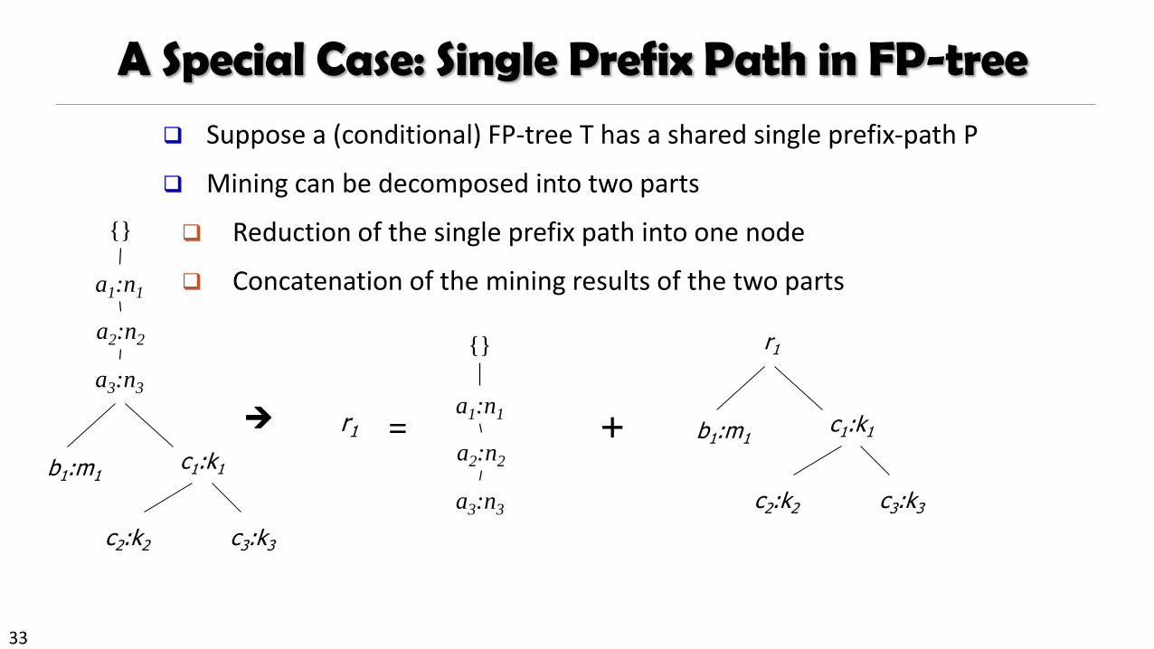
A Special Case: Single Prefix Path in FP-tree

Suppose a (conditional) FP-tree T has a shared single prefix-path P

Mining can be decomposed into two parts

Reduction of the single prefix path into one node

Concatenation of the mining results of the two parts

a2:n2

a3:n3

a1:n1

{}

b1:m1c1:k1

c2:k2 c3:k3

b1:m1c1:k1

c2:k2 c3:k3

r1

+a2:n2

a3:n3

a1:n1

{}

r1 =

34

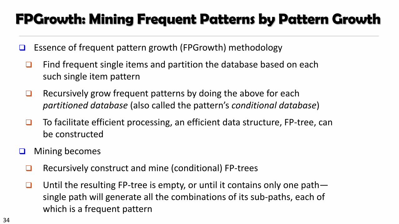
FPGrowth: Mining Frequent Patterns by Pattern Growth

Essence of frequent pattern growth (FPGrowth) methodology

Find frequent single items and partition the database based on each such single item pattern

Recursively grow frequent patterns by doing the above for each partitioned database (also called the pattern’s conditional database)

To facilitate efficient processing, an efficient data structure, FP-tree, can be constructed

Mining becomes

Recursively construct and mine (conditional) FP-trees

Until the resulting FP-tree is empty, or until it contains only one path—single path will generate all the combinations of its sub-paths, each of which is a frequent pattern

35

Assume only f’s are frequent & the frequent item ordering is: f1-f2-f3-f4

Scaling FP-growth by Item-Based Data Projection

What if FP-tree cannot fit in memory?—Do not construct FP-tree

“Project” the database based on frequent single items

Construct & mine FP-tree for each projected DB

Parallel projection vs. partition projection

Parallel projection: Project the DB on each frequent item

Space costly, all partitions can be processed in parallel

Partition projection: Partition the DB in order

Passing the unprocessed parts to subsequent partitions

f2 f3 f4 g h

f3 f4 i j

f2 f4 k

f1 f3 h

…

Trans. DB Parallel projection

f2 f3

f3

f2

…

f4-proj. DB f3-proj. DB f4-proj. DB

f2

f1

…

Partition projection

f2 f3

f3

f2

…

f1

…

f3-proj. DB

f2 will be projected to f3-proj. DB only when processing f4-proj. DB

36

CLOSET+: Mining Closed Itemsets by Pattern-Growth

Efficient, direct mining of closed itemsets

Intuition:

If an FP-tree contains a single branch as shown left

“a1,a2, a3” should be merged

Itemset merging: If Y appears in every occurrence of X, then Y is merged with X

d-proj. db: {acef, acf} → acfd-proj. db: {e}

Final closed itemset: acfd:2

There are many other tricks developed

For details, see J. Wang, et al,, “CLOSET+: Searching for the Best Strategies for Mining Frequent Closed Itemsets”, KDD'03

TID Items

1 acdef

2 abe

3 cefg

4 acdf

Let minsupport = 2

a:3, c:3, d:2, e:3, f:3

F-List: a-c-e-f-d

a2:n1

a3:n1

a1:n1

{}

b1:m1c1:k1

c2:k2 c3:k3

37


Basic Concepts


Pattern Evaluation

Summary

38

Pattern Evaluation

Limitation of the Support-Confidence Framework

Interestingness Measures: Lift and χ2

Null-Invariant Measures

Comparison of Interestingness Measures

39

How to Judge if a Rule/Pattern Is Interesting?

Pattern-mining will generate a large set of patterns/rules

Not all the generated patterns/rules are interesting

Interestingness measures: Objective vs. subjective

Objective interestingness measures

Support, confidence, correlation, …

Subjective interestingness measures:

Different users may judge interestingness differently

Let a user specify

Query-based: Relevant to a user’s particular request

Judge against one’s knowledge-base

unexpected, freshness, timeliness

40

Limitation of the Support-Confidence Framework

Are s and c interesting in association rules: “A B” [s, c]?

Example: Suppose one school may have the following statistics on # of students who may play basketball and/or eat cereal:

Association rule mining may generate the following:

play-basketball eat-cereal [40%, 66.7%] (higher s & c)

But this strong association rule is misleading: The overall % of students eating cereal is 75% > 66.7%, a more telling rule:

¬ play-basketball eat-cereal [35%, 87.5%] (high s & c)

play-basketball not play-basketball sum (row)

eat-cereal 400 350 750

not eat-cereal 200 50 250

sum(col.) 600 400 1000

Be careful!

41

Interestingness Measure: Lift

Measure of dependent/correlated events: lift

33.11000/2501000/600

1000/200),(

CBlift

89.01000/7501000/600

1000/400),(

CBlift

)()(

)(

)(

)(),(

CsBs

CBs

Cs

CBcCBlift

B ¬B ∑row

C 400 350 750

¬C 200 50 250

∑col. 600 400 1000

Lift is more telling than s & c

Lift(B, C) may tell how B and C are correlated

Lift(B, C) = 1: B and C are independent

> 1: positively correlated

< 1: negatively correlated

For our example,

Thus, B and C are negatively correlated since lift(B, C) < 1;

B and ¬C are positively correlated since lift(B, ¬C) > 1

42

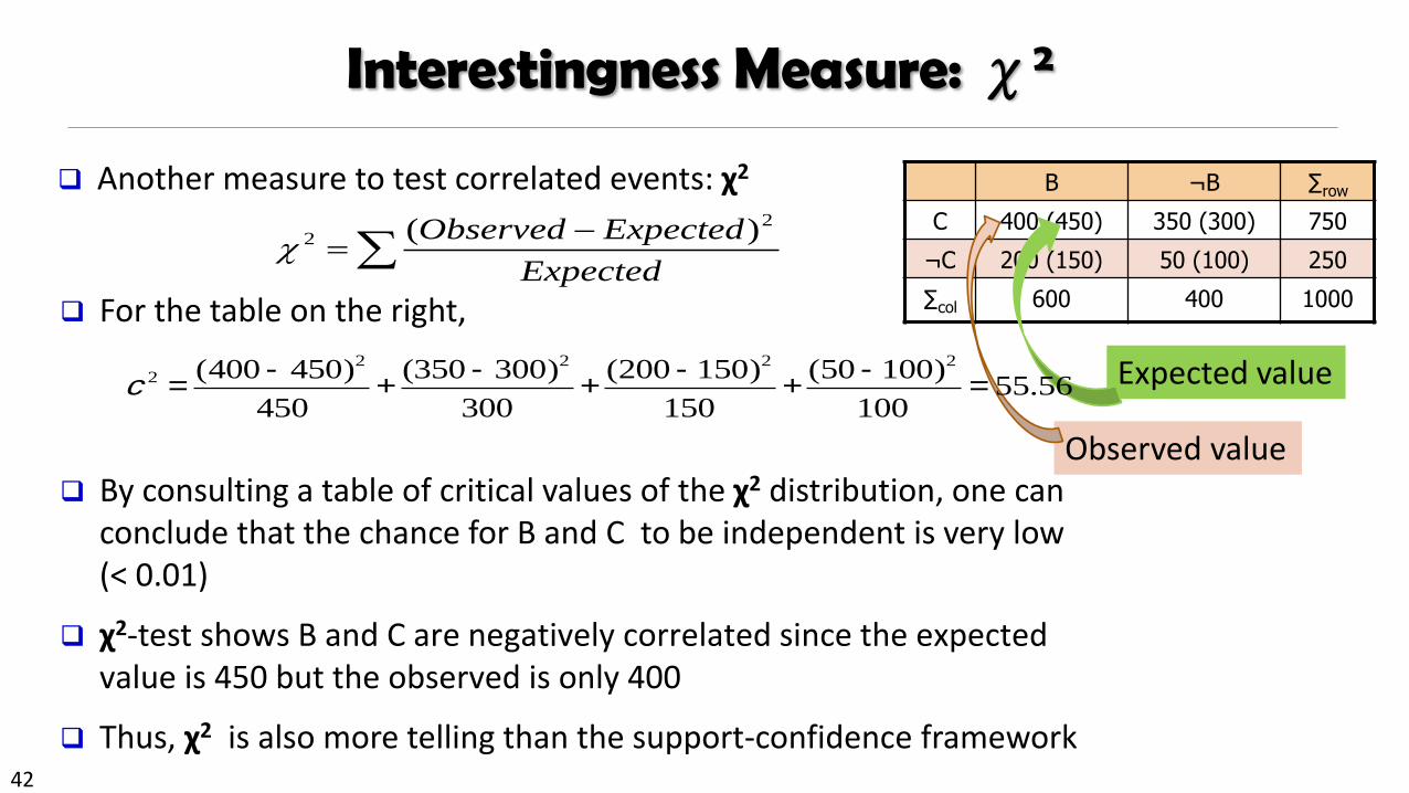
Interestingness Measure: χ2

Another measure to test correlated events: χ2B ¬B ∑row

C 400 (450) 350 (300) 750

¬C 200 (150) 50 (100) 250

∑col 600 400 1000

Expected

ExpectedObserved 22 )(

For the table on the right,

By consulting a table of critical values of the χ2 distribution, one can conclude that the chance for B and C to be independent is very low (< 0.01)

χ2-test shows B and C are negatively correlated since the expected value is 450 but the observed is only 400

Thus, χ2 is also more telling than the support-confidence framework

Expected value

Observed value

c 2 =(400 - 450)2

450+

(350 -300)2

300+

(200 -150)2

150+

(50 -100)2

100= 55.56

43

Lift and χ2 : Are They Always Good Measures?

Null transactions: Transactions that contain

neither B nor C

Let’s examine the new dataset D

BC (100) is much rarer than B¬C (1000) and ¬BC

(1000), but there are many ¬B¬C (100000)

Unlikely B & C will happen together!

But, Lift(B, C) = 8.44 >> 1 (Lift shows B and C are

strongly positively correlated!)

χ2 = 670: Observed(BC) >> expected value (11.85)

Too many null transactions may “spoil the soup”!

B ¬B ∑row

C 100 1000 1100

¬C 1000 100000 101000

∑col. 1100 101000 102100

B ¬B ∑row

C 100 (11.85) 1000 1100

¬C 1000 (988.15) 100000 101000

∑col. 1100 101000 102100

null transactions

Contingency table with expected values added

44

Interestingness Measures & Null-Invariance

Null invariance: Value does not change with the # of null-transactions

A few interestingness measures: Some are null invariant

Χ2 and lift are not null-invariant

Jaccard, consine, AllConf, MaxConf,

and Kulczynskiare null-invariant

measures

45

Null Invariance: An Important Property

Why is null invariance crucial for the analysis of massive transaction data?

Many transactions may contain neither milk nor coffee!

Lift and 2 are not null-invariant: not good to evaluate data that contain too many or too few null transactions!

Many measures are not null-invariant!

Null-transactions w.r.t. m and c

milk vs. coffee contingency table

46

Comparison of Null-Invariant Measures

Not all null-invariant measures are created equal

Which one is better?

D4—D6 differentiate the null-invariant measures

Kulc (Kulczynski 1927) holds firm and is in balance of both directional implications

All 5 are null-invariant

Subtle: They disagree on those cases

2-variable contingency table

47

Analysis of DBLP Coauthor Relationships

Which pairs of authors are strongly related?

Use Kulc to find Advisor-advisee, close collaborators

DBLP: Computer science research publication bibliographic database

> 3.8 million entries on authors, paper, venue, year, and other information

Advisor-advisee relation: Kulc: high, Jaccard: low, cosine: middle

48

Imbalance Ratio with Kulczynski Measure

IR (Imbalance Ratio): measure the imbalance of two itemsets A and B in rule implications:

Kulczynski and Imbalance Ratio (IR) together present a clear picture for all the three datasets D4 through D6

D4 is neutral & balanced; D5 is neutral but imbalanced

D6 is neutral but very imbalanced

49

What Measures to Choose for Effective Pattern Evaluation?

Null value cases are predominant in many large datasets

Neither milk nor coffee is in most of the baskets; neither Mike nor Jim is an author in most of the papers; ……

Null-invariance is an important property

Lift, χ2 and cosine are good measures if null transactions are not predominant

Otherwise, Kulczynski + Imbalance Ratio should be used to judge the interestingness of a pattern

Exercise: Mining research collaborations from research bibliographic data

Find a group of frequent collaborators from research bibliographic data (e.g., DBLP)

Can you find the likely advisor-advisee relationship and during which years such a relationship happened?

Ref.: C. Wang, J. Han, Y. Jia, J. Tang, D. Zhang, Y. Yu, and J. Guo, "Mining Advisor-Advisee Relationships from Research Publication Networks", KDD'10

50


Basic Concepts


Pattern Evaluation

Summary

51

Summary Basic Concepts

What Is Pattern Discovery? Why Is It Important?

Basic Concepts: Frequent Patterns and Association Rules

Compressed Representation: Closed Patterns and Max-Patterns



The Apriori Algorithm

Extensions or Improvements of Apriori

Mining Frequent Patterns by Exploring Vertical Data Format

FPGrowth: A Frequent Pattern-Growth Approach

Mining Closed Patterns

Pattern Evaluation

Interestingness Measures in Pattern Mining

Interestingness Measures: Lift and χ2

Null-Invariant Measures

Comparison of Interestingness Measures

52

Recommended Readings (Basic Concepts)

R. Agrawal, T. Imielinski, and A. Swami, “Mining association rules between sets of items in large databases”, in Proc. of SIGMOD'93

R. J. Bayardo, “Efficiently mining long patterns from databases”, in Proc. of SIGMOD'98

N. Pasquier, Y. Bastide, R. Taouil, and L. Lakhal, “Discovering frequent closed itemsetsfor association rules”, in Proc. of ICDT'99

J. Han, H. Cheng, D. Xin, and X. Yan, “Frequent Pattern Mining: Current Status and Future Directions”, Data Mining and Knowledge Discovery, 15(1): 55-86, 2007

53

Recommended Readings (Efficient Pattern Mining Methods)

R. Agrawal and R. Srikant, “Fast algorithms for mining association rules”, VLDB'94

A. Savasere, E. Omiecinski, and S. Navathe, “An efficient algorithm for mining association rules in large databases”, VLDB'95

J. S. Park, M. S. Chen, and P. S. Yu, “An effective hash-based algorithm for mining association rules”, SIGMOD'95

S. Sarawagi, S. Thomas, and R. Agrawal, “Integrating association rule mining with relational database systems: Alternatives and implications”, SIGMOD'98

M. J. Zaki, S. Parthasarathy, M. Ogihara, and W. Li, “Parallel algorithm for discovery of association rules”, Data Mining and Knowledge Discovery, 1997

J. Han, J. Pei, and Y. Yin, “Mining frequent patterns without candidate generation”, SIGMOD’00

M. J. Zaki and Hsiao, “CHARM: An Efficient Algorithm for Closed Itemset Mining”, SDM'02

J. Wang, J. Han, and J. Pei, “CLOSET+: Searching for the Best Strategies for Mining Frequent Closed Itemsets”, KDD'03

C. C. Aggarwal, M.A., Bhuiyan, M. A. Hasan, “Frequent Pattern Mining Algorithms: A Survey”, in Aggarwal and Han (eds.): Frequent Pattern Mining, Springer, 2014

54

Recommended Readings (Pattern Evaluation)

C. C. Aggarwal and P. S. Yu. A New Framework for Itemset Generation. PODS’98

S. Brin, R. Motwani, and C. Silverstein. Beyond market basket: Generalizing association rules to correlations. SIGMOD'97

M. Klemettinen, H. Mannila, P. Ronkainen, H. Toivonen, and A. I. Verkamo. Finding interesting rules from large sets of discovered association rules. CIKM'94

E. Omiecinski. Alternative Interest Measures for Mining Associations. TKDE’03

P.-N. Tan, V. Kumar, and J. Srivastava. Selecting the Right Interestingness Measure for Association Patterns. KDD'02

T. Wu, Y. Chen and J. Han, Re-Examination of Interestingness Measures in Pattern Mining: A Unified Framework, Data Mining and Knowledge Discovery, 21(3):371-397, 2010

55October 1, 2017 Data Mining: Concepts and Techniques

Documents

CS 412 Intro. to Data Mining - University Of Illinoisweb.engr.illinois.edu/~hanj/cs412/bk3_slides/06FPBasic.pdf · CS 412 Intro. to Data Mining Chapter 6. ... Ex. sup{Beer, Eggs}