CS 345:Topics in Data Warehousing

Tuesday, November 2, 2004

Review of Thursday’s Class

• Join Indexes

• Projection Indexes– Horizontal vs. Vertical decomposition

• Bit-Sliced Indexes– Fast bitmap counts and sums– Range queries

• Bit Vector Filtering

Outline of Today’s Class

• Pre-computed aggregates– Materialized views– Aggregate navigation– Dimension and fact aggregates

• Selection of aggregates– Manual selection– Greedy algorithm– Limitations of greedy approach

Physical Database Design

• Logical database design– What are the facts and dimensions?– Goals: Simplicity, Expressiveness– Make the database easy to understand– Make queries easy to ask

• Physical database design– How should the data be arranged on disk?– Goal: Performance

• Manageability is an important secondary concern

– Make queries run fast

Load vs. Query Trade-off

• Trade-off between query performance and load performance

• To make queries run fast:– Precompute as much as possible– Build lots of data structures

• Indexes• Materialized views

• But…– Data structures require disk space to store– Building/updating data structures takes time– More data structures → longer load time

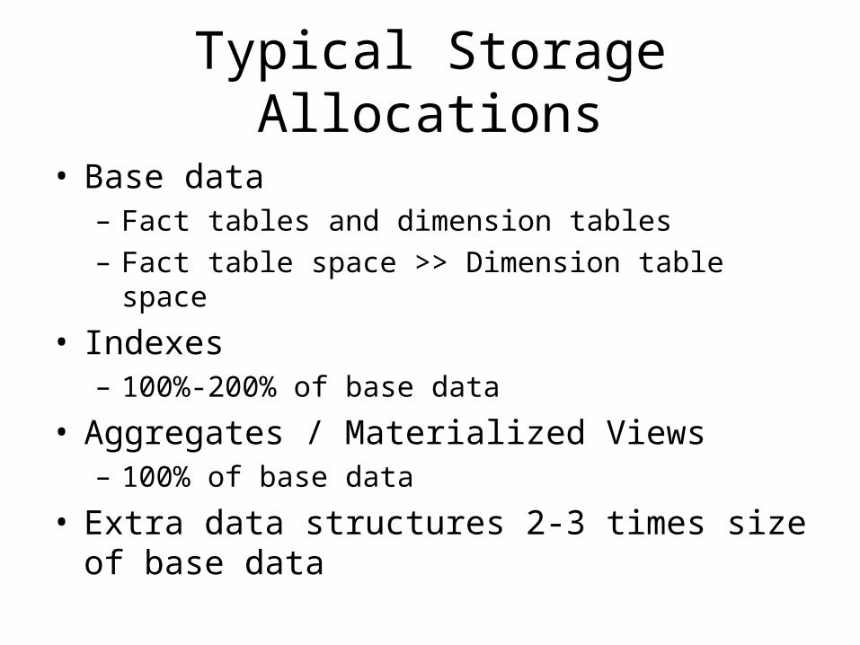
Typical Storage Allocations

• Base data– Fact tables and dimension tables– Fact table space >> Dimension table space

• Indexes– 100%-200% of base data

• Aggregates / Materialized Views– 100% of base data

• Extra data structures 2-3 times size of base data

Materialized Views

• Many DBMSs support materialized views– Precomputed result of a particular query– Goal: faster response for related queries

• Example:– View definition:SELECT State, SUM(Quantity) FROM Sales GROUP BY State

– Query: SELECT SUM(Quantity) FROM SalesWHERE State = 'CA'

– Scan view rather than Sales table• View matching problem

– When can a query be re-written using a materialized view?– Difficult to solve in its full generality– DBMSs handle common cases via limited set of re-write rules

Aggregate Tables

• Also known as summary tables• Common form of precomputation in data

warehouses• Reduce dimensionality of fact by

aggregating across some dimensions– Result is smaller version of fact table

• Can be used to answer queries that refer only to dimensions that are retained– Similar to the idea of a covering index

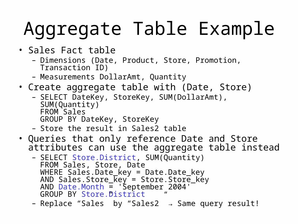
Aggregate Table Example• Sales Fact table

– Dimensions (Date, Product, Store, Promotion, Transaction ID)– Measurements DollarAmt, Quantity

• Create aggregate table with (Date, Store)– SELECT DateKey, StoreKey, SUM(DollarAmt), SUM(Quantity)FROM SalesGROUP BY DateKey, StoreKey

– Store the result in Sales2 table• Queries that only reference Date and Store attributes

can use the aggregate table instead– SELECT Store.District, SUM(Quantity)FROM Sales, Store, DateWHERE Sales.Date_key = Date.Date_keyAND Sales.Store_key = Store.Store_keyAND Date.Month = 'September 2004'GROUP BY Store.District

– Replace “Sales” by “Sales2” → Same query result!

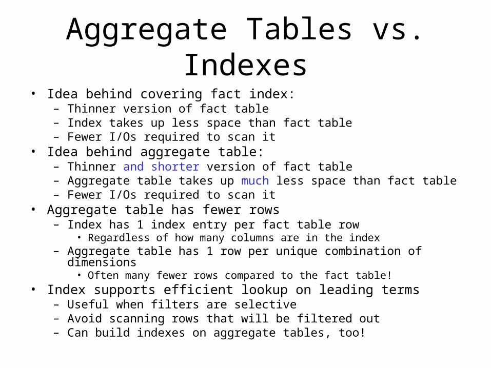
Aggregate Tables vs. Indexes• Idea behind covering fact index:

– Thinner version of fact table– Index takes up less space than fact table– Fewer I/Os required to scan it

• Idea behind aggregate table:– Thinner and shorter version of fact table– Aggregate table takes up much less space than fact table– Fewer I/Os required to scan it

• Aggregate table has fewer rows– Index has 1 index entry per fact table row

• Regardless of how many columns are in the index– Aggregate table has 1 row per unique combination of dimensions

• Often many fewer rows compared to the fact table!• Index supports efficient lookup on leading terms

– Useful when filters are selective– Avoid scanning rows that will be filtered out– Can build indexes on aggregate tables, too!

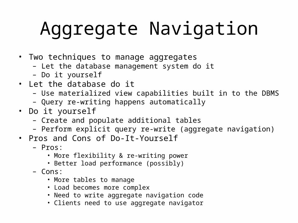
Aggregate Navigation• Two techniques to manage aggregates

– Let the database management system do it– Do it yourself

• Let the database do it– Use materialized view capabilities built in to the DBMS– Query re-writing happens automatically

• Do it yourself– Create and populate additional tables – Perform explicit query re-write (aggregate navigation)

• Pros and Cons of Do-It-Yourself– Pros:

• More flexibility & re-writing power• Better load performance (possibly)

– Cons: • More tables to manage• Load becomes more complex• Need to write aggregate navigation code• Clients need to use aggregate navigator

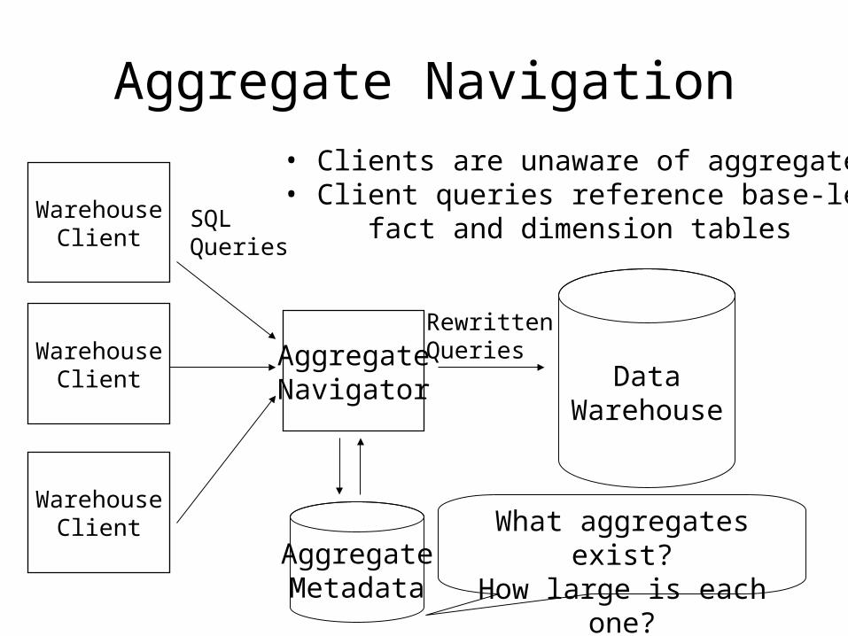
Aggregate Navigation

WarehouseClient

AggregateNavigator

SQLQueries

DataWarehouse

AggregateMetadata

WarehouseClient

WarehouseClient

RewrittenQueries

What aggregates exist?How large is each one?

• Clients are unaware of aggregates• Client queries reference base-level fact and dimension tables

Dimension Aggregates• Methods to define aggregates

– 1. Include or leave out entire dimensions– 2. Include some columns of each dimension, but not others– Second approach is more common / more useful

• Example: Several versions of Date dimension– Base Date dimension

• 1 row per day• Includes all Date attributes

– Monthly aggregate dimension• 1 row per month• Includes Date attributes at month level or higher

– Yearly aggregate dimension• 1 row per year• Includes only year-level Date attributes

• Each dimension aggregate has its own set of surrogate keys• Each aggregated fact joins to 1 version of the Date dimension

– Or else the Date dimension is omitted entirely…

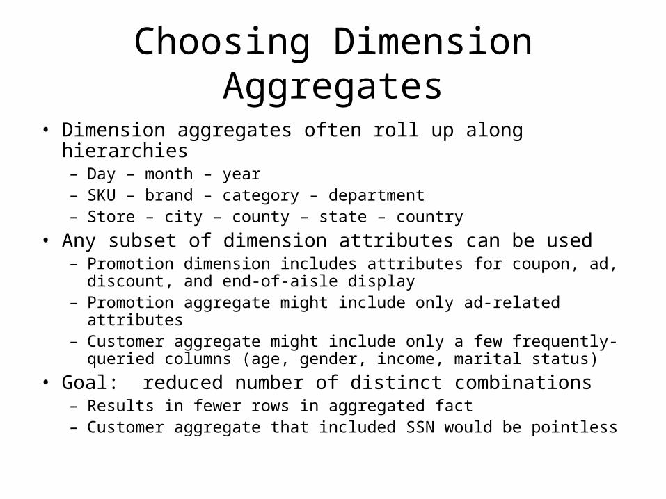
Choosing Dimension Aggregates

• Dimension aggregates often roll up along hierarchies– Day – month – year– SKU – brand – category – department– Store – city – county – state – country

• Any subset of dimension attributes can be used– Promotion dimension includes attributes for coupon, ad,

discount, and end-of-aisle display– Promotion aggregate might include only ad-related attributes– Customer aggregate might include only a few frequently-queried

columns (age, gender, income, marital status)

• Goal: reduced number of distinct combinations– Results in fewer rows in aggregated fact– Customer aggregate that included SSN would be pointless

Aggregate Examples• Sales fact table

– Date, Product, Store, Promotion, Transaction ID• Date aggregates

– Month– Year

• Product aggregates– Brand– Manufacturer

• Promotion aggregates– Ad– Discount– Coupon– In-Store Display

• Store aggregates– District– State

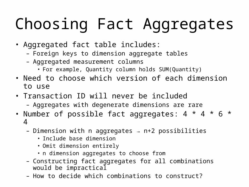
Choosing Fact Aggregates• Aggregated fact table includes:

– Foreign keys to dimension aggregate tables– Aggregated measurement columns

• For example, Quantity column holds SUM(Quantity)

• Need to choose which version of each dimension to use• Transaction ID will never be included

– Aggregates with degenerate dimensions are rare

• Number of possible fact aggregates: 4 * 4 * 6 * 4– Dimension with n aggregates → n+2 possibilities

• Include base dimension• Omit dimension entirely• n dimension aggregates to choose from

– Constructing fact aggregates for all combinations would be impractical

– How to decide which combinations to construct?

Aggregate Selection• Two approaches

– Manual selection• Data warehouse designer chooses aggregates• Could be time-consuming and error-prone

– Automatic selection• Use algorithms to optimize choice of aggregates• Good in principle; however, problem is hard

• Heuristics for manual selection– Include a mixture of breadth and depth

• A few broad aggregates – Lots of dimensions at fairly fine-grained level of detail– Achieve moderate speedup on a wide range of queries

• Lots of highly targeted aggregates with only a few rows each– Dimensions are highly rolled up or omitted entirely– Each aggregate achieves large speedup on a small class of queries

• Roughly equal allocation of space to each type– Consider the query workload

• What attributes are queried most frequently?• What sets of attributes are often queried together?• Make sure that common / important queries run fast• Aggregate design can be adjusted over time (learn from experience)

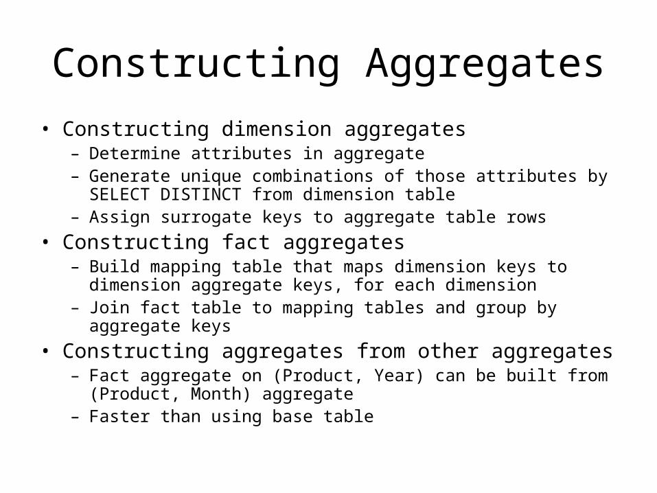
Constructing Aggregates

• Constructing dimension aggregates– Determine attributes in aggregate– Generate unique combinations of those attributes by SELECT

DISTINCT from dimension table– Assign surrogate keys to aggregate table rows

• Constructing fact aggregates– Build mapping table that maps dimension keys to dimension

aggregate keys, for each dimension– Join fact table to mapping tables and group by aggregate keys

• Constructing aggregates from other aggregates– Fact aggregate on (Product, Year) can be built from (Product,

Month) aggregate– Faster than using base table

Data Cube Lattice

Total

State Month Color

State, Month

State,Color

Month,Color

State, Month, Color

DrillDown

RollUp

Sparsity Revisited

• Fact tables are usually sparse– Not all possible combinations of dimension values actually occur– E.g. not all products sell in all stores on all days

• Aggregate tables are not as sparse– Coarser grain → lesser sparsity– All products sell in SOME store in all MONTHS– Thus space savings from aggregation can be less than one

might think• Example: Date dimension vs. Year dimension aggregate

– Year table has 1/365 as many rows as Date table– Fact aggregate with (Product, Store, Year) has fewer rows than

fact aggregate with (Product, Store, Date)– But more than 1/365 of the rows!– Some potential space savings are lost due to reduced sparsity

Automatic Selection of Aggregates

• Problem Definition– Inputs:

• Query workload• Set of candidate aggregates• Query cost model• Maximum space to use for aggregates

– Output:• Set of aggregates to construct

– Objective:• Minimize cost of executing query workload

• Problem is NP-Complete– Approximation is required– We’ll discuss a Greedy algorithm for the problem– Due to Harinarayan, Rajaraman, and Ullman (1996)

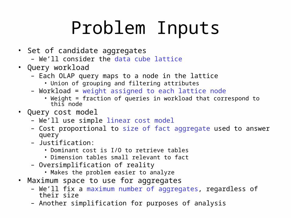
Problem Inputs• Set of candidate aggregates

– We’ll consider the data cube lattice• Query workload

– Each OLAP query maps to a node in the lattice• Union of grouping and filtering attributes

– Workload = weight assigned to each lattice node• Weight = fraction of queries in workload that correspond to this node

• Query cost model– We’ll use simple linear cost model– Cost proportional to size of fact aggregate used to answer query– Justification:

• Dominant cost is I/O to retrieve tables• Dimension tables small relevant to fact

– Oversimplification of reality• Makes the problem easier to analyze

• Maximum space to use for aggregates– We’ll fix a maximum number of aggregates, regardless of their size– Another simplification for purposes of analysis

Configurations

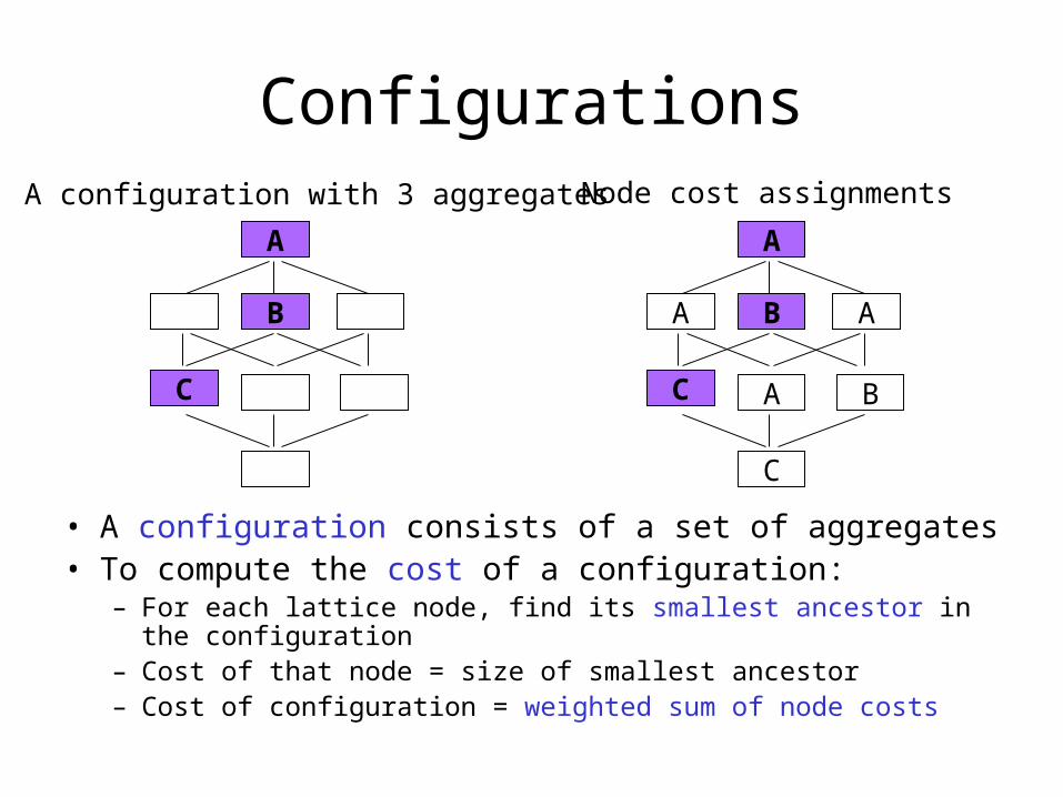
• A configuration consists of a set of aggregates• To compute the cost of a configuration:

– For each lattice node, find its smallest ancestor in the configuration

– Cost of that node = size of smallest ancestor– Cost of configuration = weighted sum of node costs

C

B

A

C

C A B

A B A

A

A configuration with 3 aggregates Node cost assignments

Greedy Algorithm

• Greedy aggregate selection algorithm– Add aggregates one at a time until space budget is exhausted– Always add the aggregate whose addition will most decrease the

cost of the current configuration

• Performance guarantee for Greedy– Benefit of configuration C =(cost of no-aggregate configuration) -

(cost of C)– BG,k = Benefit of k-aggregate configuration chosen by greedy

algorithm– BOPT,k = Benefit of best possible k-aggregate configuration– Theorem: BG,k > BOPT,k *0.63

• Greedy always achieves at least 63% of optimal benefit• For proof, see “Implementing Data Cubes Efficiently”, by

Harinarayan, Rajaraman, and Ullman, 1996

Example of Greedy Algorithm

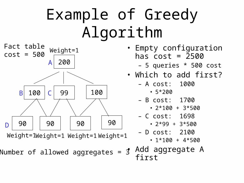
• Empty configuration has cost = 2500– 5 queries * 500 cost

• Which to add first?– A cost: 1000

• 5*200

– B cost: 1700• 2*100 + 3*500

– C cost: 1698• 2*99 + 3*500

– D cost: 2100• 1*100 + 4*500

• Add aggregate A first

9090 90 90

100 99 100

200

Weight=1 Weight=1 Weight=1 Weight=1

Fact table cost = 500

Number of allowed aggregates = 3

A

B C

D

Weight=1

Example of Greedy Algorithm

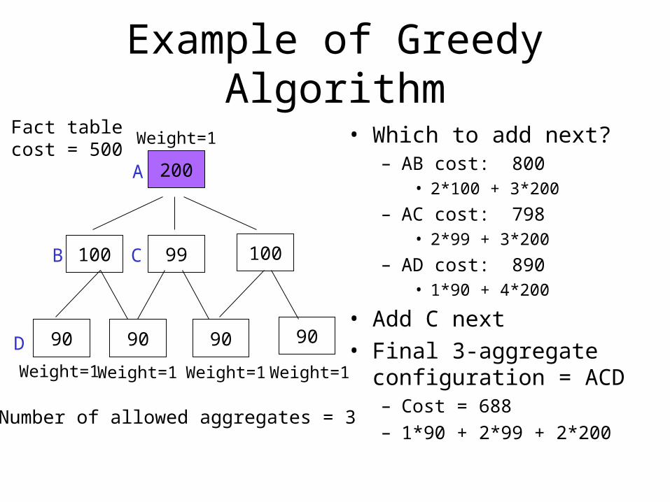
• Which to add next?– AB cost: 800

• 2*100 + 3*200

– AC cost: 798• 2*99 + 3*200

– AD cost: 890• 1*90 + 4*200

• Add C next• Final 3-aggregate

configuration = ACD– Cost = 688– 1*90 + 2*99 + 2*200

9090 90 90

100 99 100

200

Weight=1 Weight=1 Weight=1 Weight=1

Fact table cost = 500

Number of allowed aggregates = 3

A

B C

D

Weight=1

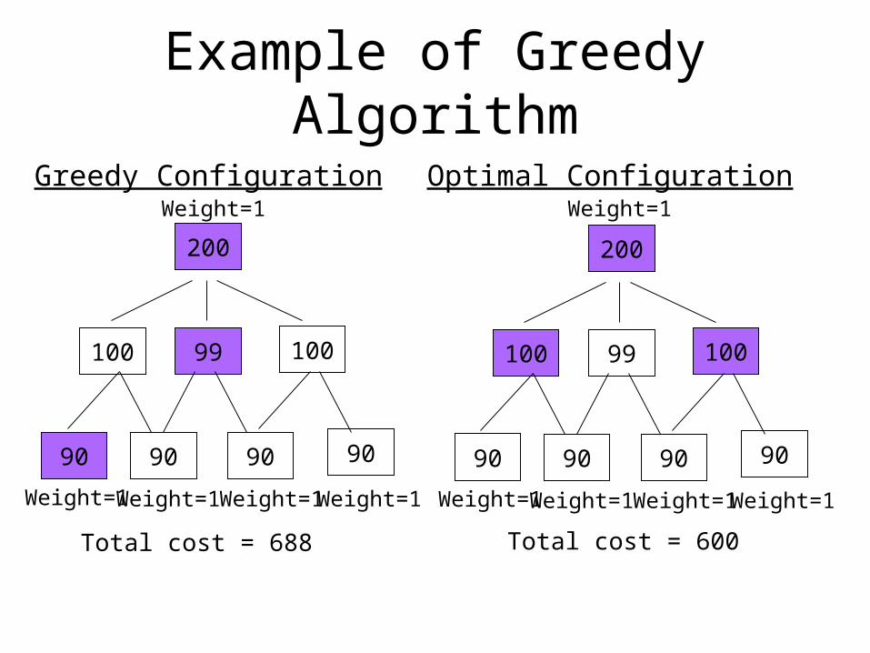
Example of Greedy Algorithm

9090 90 90

100 99 100

200

Weight=1Weight=1 Weight=1 Weight=1

Greedy Configuration

Total cost = 688

9090 90 90

100 99 100

200

Weight=1Weight=1 Weight=1 Weight=1

Optimal ConfigurationWeight=1 Weight=1

Total cost = 600

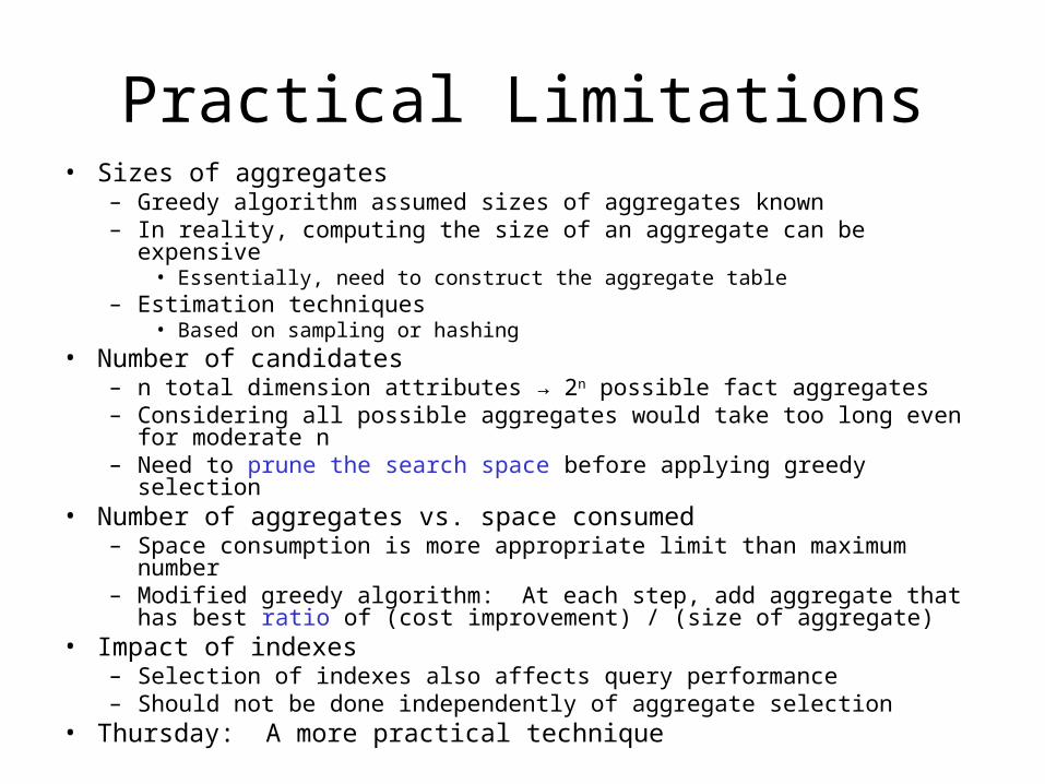
Practical Limitations• Sizes of aggregates

– Greedy algorithm assumed sizes of aggregates known – In reality, computing the size of an aggregate can be expensive

• Essentially, need to construct the aggregate table– Estimation techniques

• Based on sampling or hashing• Number of candidates

– n total dimension attributes → 2n possible fact aggregates– Considering all possible aggregates would take too long even for

moderate n– Need to prune the search space before applying greedy selection

• Number of aggregates vs. space consumed– Space consumption is more appropriate limit than maximum number– Modified greedy algorithm: At each step, add aggregate that has best

ratio of (cost improvement) / (size of aggregate)• Impact of indexes

– Selection of indexes also affects query performance– Should not be done independently of aggregate selection

• Thursday: A more practical technique

Course Project

• Project is deliberately open-ended• Some possibilities include:

– Survey of research literature• Read several related research papers & write a report summarizing

them– Research project

• Compare alternate approaches to the same problem• Devise and test a brand new approach to a difficult problem

– Programming project• Build a tool for some aspect of designing / querying / loading data

warehouses• Implement one of the data structures or algorithms discussed in

class– Other project related to your research / interests

• Should involve concepts from this course in some way

Course Project

• Project timeline– By Tuesday, Nov. 9:

• Send the instructor e-mail with the general topic you’re considering• It’s OK if you don’t yet know exactly what you want to do• Receive feedback to help narrow in on a specific project

– By Tuesday, Nov. 16:• Submit project description (1 page or less)• Describe your plans in some detail

– Tuesday, Nov. 30 and Tuesday, Dec. 2:• 5-10 minute in-class presentations• Brief overview of your project and your results• Doing a demo is great, if appropriate

– By Wednesday, Dec. 8:• Submit final project write-up