Issues in Scaling Up the 700 MHz Auction Design

Second FCC Combinatorial Auction ConferenceOctober 27, 2001

CS 286r. Computational Mechanism Design

Thanks for Karla Hoffman, GMU, for allowing use of these slides

Issues in Scaling Up the 700 MHz Auction Design

Wye River Conference II October 27, 2001

Melissa Dunford Martin Durbin Karla Hoffman Dinesh Menon Rudy Sultana Thomas Wilson

Introduction Auction #31 rules were designed specifically for

that auction– No computational problems for a 12 license auction

Seeking a design for large combinatorial auctions– Start with Auction #31, identify the problem areas in

regards to scalability and then discuss alternatives

Outline

Review of Auction #31 rules impacting scalability and possible alternatives– Determining maximum revenue each round– Choosing among ties– Minimum Acceptable Bid (MAB)

Mechanism for testing scalability

Auction #31 Formulation Choose among a set of bids such that:

– Revenue to the FCC is maximized– Each license is awarded exactly once – No bidder has bids in a provisionally winning bid set from more than one round

subject to:

Ax = 1 (each license awarded exactly once)

Mutually Exclusive Bid Constraints

Bids

bbb

xxBidAmtMax

#

1

bidsallforxb 1,0

Ax =1: Each license awarded once

This is called a set-partitioning problem. These types of problems have a very nice mathematical structure.

Bid

Bid amt.

2

$12e6

3

$30e6$22e6

1 4

$16e6

5

$8e6

Package B ABCABD AD C

6

$11e6

BC

7

$10e6

A

8

$7e6

D

x3 + x5 + x6

+ x3x1 + x4 + x7

x1 + x4 + x8

B

C

A

D

= 1

= 1

= 1

= 1

+ x2 + x3x1 + x6

0 11 1 0 0 1 0

1 11 0 0 1 0 0

0 10 0 1 1 0 0

0 01 1 0 0 0 1

Example: 4 licenses, 8 bids

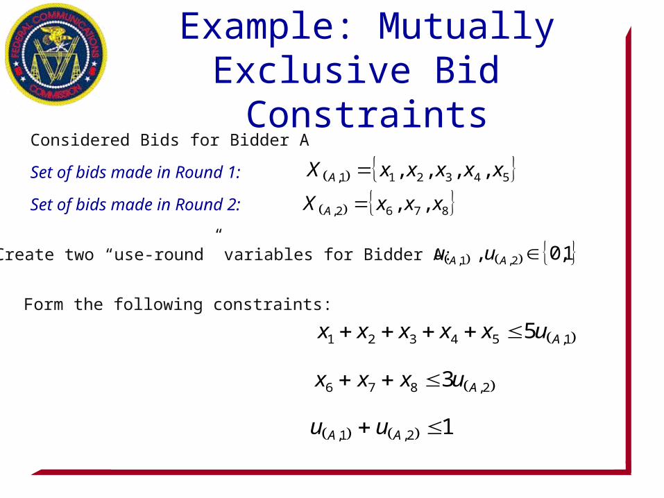
Example: Mutually Exclusive Bid Constraints

Considered Bids for Bidder A

Set of bids made in Round 1:

Set of bids made in Round 2:

543211, ,,,, xxxxxX A

8762, ,, xxxX A

1,0, 2,1, AA uuCreate two “use-round” variables for Bidder A:

12,1, AA uu

Form the following constraints:

1,54321 5 Auxxxxx

2,876 3 Auxxx

Mutually exclusive bid constraints alter the nice structure of set-partitioning (Ax =1) and make the problem harder to solve

Solving Challenges: Mutually Exclusive Bid Rule

x3 + x5 + x6

+ x3x1 + x4 + x7

x1 + x4 + x8

B

C

A

D

= 1

= 1

= 1

= 1

+ x2 + x3x1 + x6

R(A,2)

UA

R(A,1)

0

1

<=

<=

<=

0

+ u(A,2)

+ x2 + x3x1 + x4 + x5

+ x6 + x7 + x8

u(A,1)

- 3u(A,2)

- 5u(A,1)

0 11 1 0 0 1 0

1 11 0 0 1 0 0

0 10 0 1 1 0 0

0 01 1 0 0 0 1

1 0

0 0

0 0

0 1

1 11 1 1 0 0 0

0 00 0 0 1 1 1

0 00 0 0 0 0 0

-5 0

0 -3

1 1

Solvability of Integer Optimizations

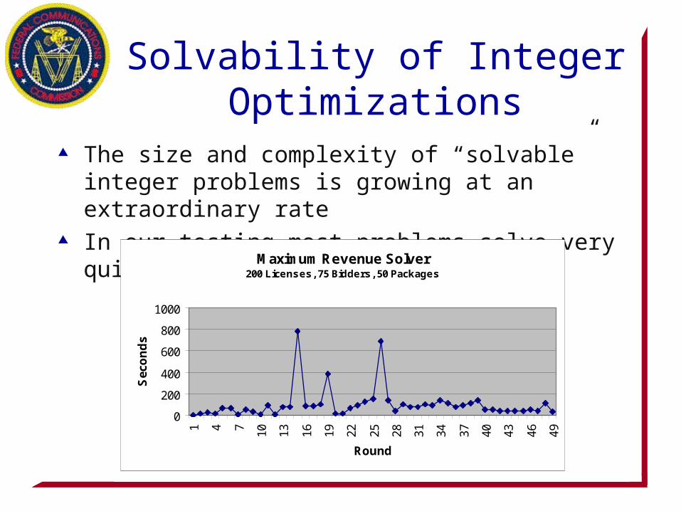
The size and complexity of “solvable” integer problems is growing at an extraordinary rate

In our testing most problems solve very quickly, but...

Maximum Revenue Solver200 Licenses, 75 Bidders, 50 Packages

0

200

400

600

800

1000

1 4 7 10 13 16 19 22 25 28 31 34 37 40 43 46 49

Round

Sec

on

ds

Breaking Ties

Solvers work at getting an optimal solution quickly, no solver automatically provides tie information

Breaking ties randomly important for legal reasons Cannot use a tie-breaking method that requires the

generation of all tied sets (there could be millions of tied sets even for an auction with few licenses)

Tie-Breaking Procedure

Ties will be broken randomly using a two-step process– First step selects a bid set that achieves the

maximum revenue– Second step selects a bid set at random from all

optimal bid sets

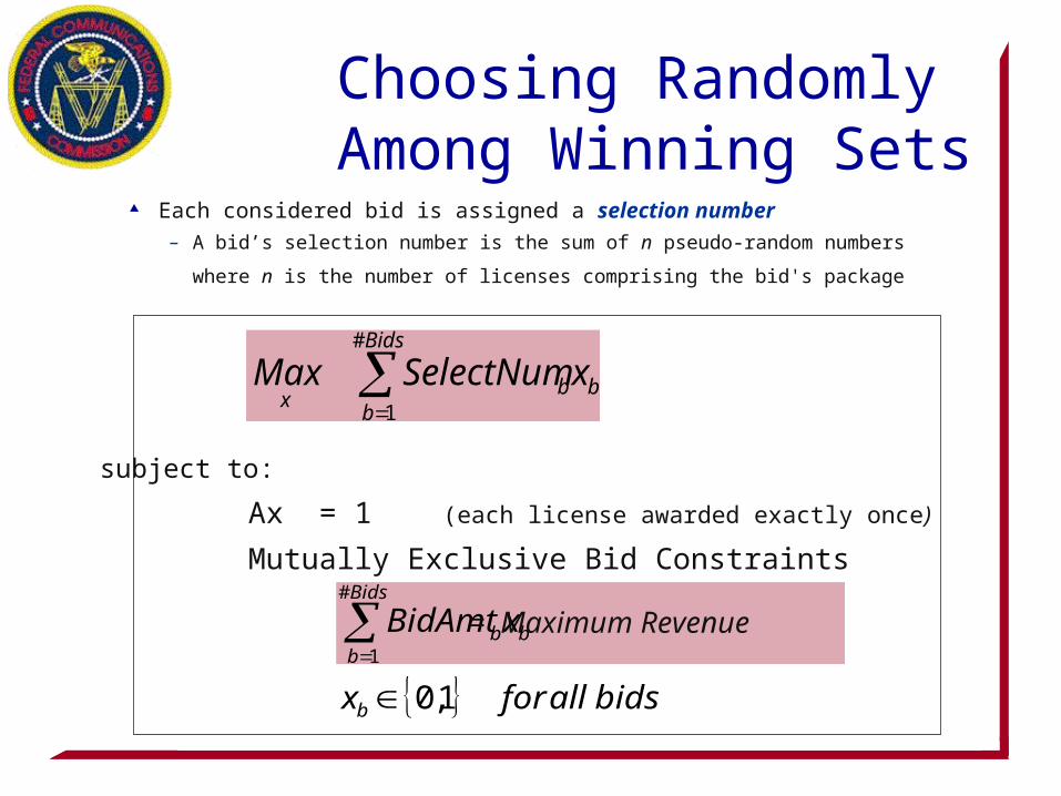
Each considered bid is assigned a selection number

– A bid’s selection number is the sum of n pseudo-random numbers where n is the

number of licenses comprising the bid's package

Choosing Randomly Among Winning Sets

Bids

bbb xBidAmt

#

1

bidsallforxb 1,0

Bids

bbb

xxSelectNumMax

#

1

subject to:

Ax = 1 (each license awarded exactly once)

Mutually Exclusive Bid Constraints

= Maximum Revenue

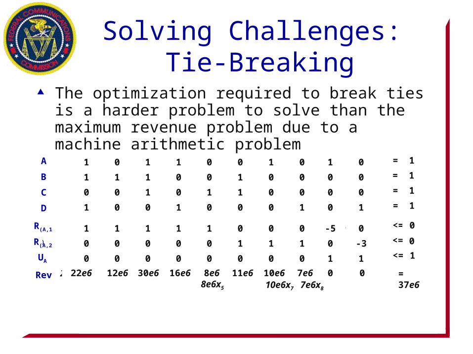
+ 12e6x2 + 30e6x322e6x1 + 16e6x4 + 8e6x5 + 11e6x6+ 10e6x7 + 7e6x8 = 37e6

+ u(A,2)

+ x2 + x3x1 + x4 + x5

+ x6 + x7 + x8

u(A,1)

- 3u(A,2)

- 5u(A,1)

x3 + x5 + x6

+ x3x1 + x4 + x7

x1 + x4 + x8

B

C

A

D

= 1

= 1

= 1

= 1

+ x2 + x3x1 + x6

Rev

0

1

<=

<=

<=

0

R(A,2)

UA

R(A,1)

The optimization required to break ties is a harder problem to solve than the maximum revenue problem due to a machine arithmetic problem

Solving Challenges: Tie-Breaking

0 11 1 0 0 1 0

1 11 0 0 1 0 0

0 10 0 1 1 0 0

0 01 1 0 0 0 1

1 0

0 0

0 0

0 1

1 11 1 1 0 0 0

0 00 0 0 1 1 1

0 00 0 0 0 0 0

-5 0

0 -3

1 1

12 3022 16 8 11 10 7 0 022e6 = 37e612e6 30e6 16e6 8e6 11e6 10e6 7e6 0 0

Tie-Breaking: Evaluation

Current method of random tie-breaking works Due to time considerations in large auctions, tie-breaking

procedure may be postponed until later rounds

– Concept of stages

Minimum Acceptable Bids

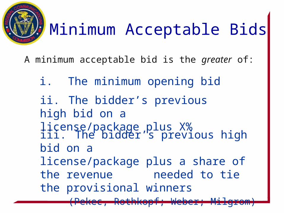
A minimum acceptable bid is the greater of:

i. The minimum opening bid

ii. The bidder’s previous high bid on a license/package plus X%

iii. The bidder’s previous high bid on a license/package plus a share of the

revenue needed to tie the provisional winners

(Pekec, Rothkopf; Weber; Milgrom)

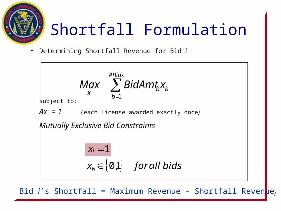
Shortfall Formulation Determining Shortfall Revenue for Bid i

subject to:

Ax = 1 (each license awarded exactly once)

Mutually Exclusive Bid Constraints

Bids

bbb

xxBidAmtMax

#

1

bidsallforxb 1,0

1ix

Bid i’s Shortfall = Maximum Revenue - Shortfall Revenuei

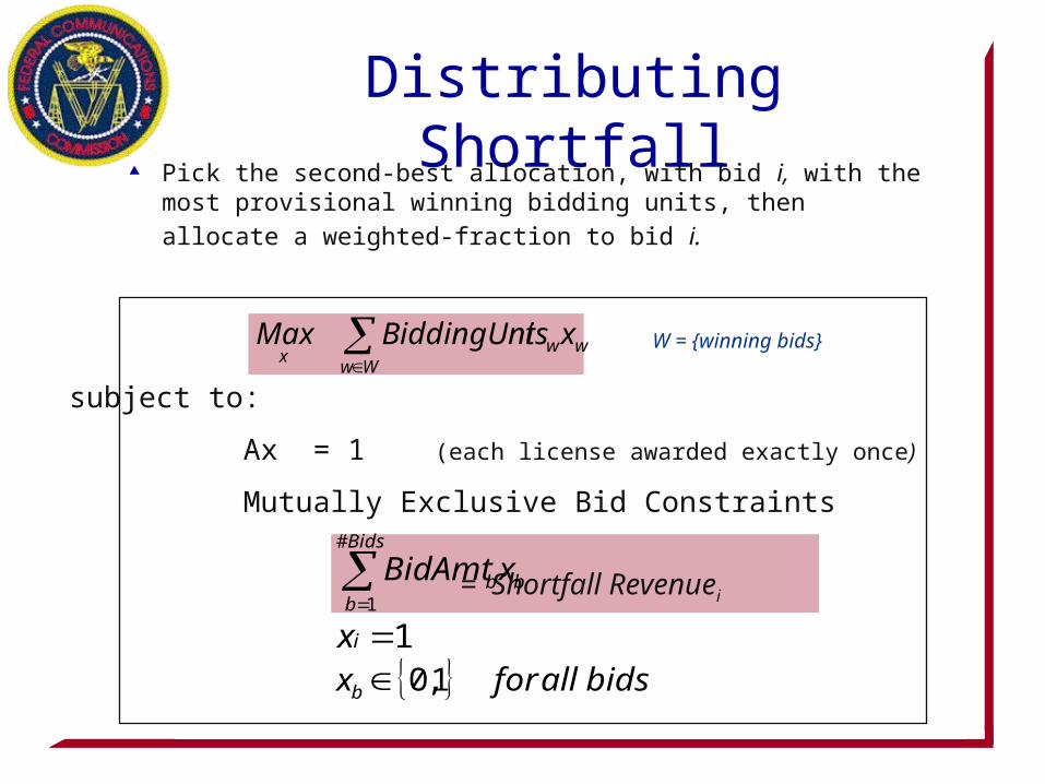
Distributing Shortfall Pick the second-best allocation, with bid i, with the most

provisional winning bidding units, then allocate a weighted-

fraction to bid i.there can be more

subject to:

Ax = 1 (each license awarded exactly once)

Mutually Exclusive Bid Constraints

= Shortfall Revenuei

Bids

bbb xBidAmt

#

1

bidsallforxb 1,0

Ww

wwx

xtsBiddingUniMax

1ix

W = {winning bids}

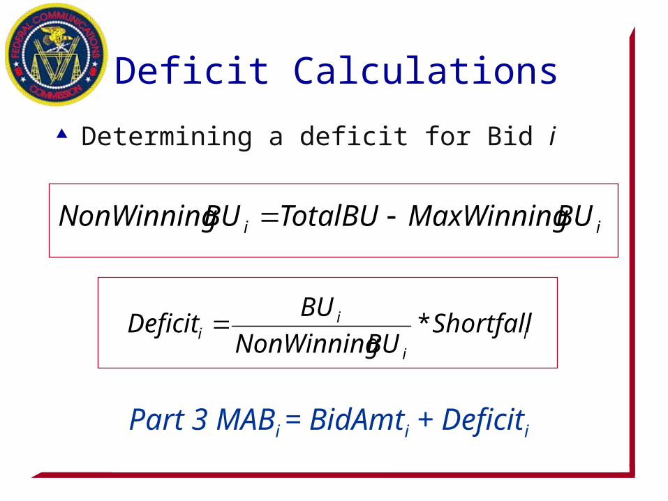
Deficit Calculations

Determining a deficit for Bid i

Part 3 MABi = BidAmti + Deficiti

ii BUMaxWinningTotalBUBUNonWinning

ii

ii Shortfall

BUNonWinning

BUDeficit *

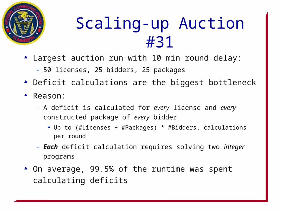
Scaling-up Auction #31

Largest auction run with 10 min round delay:

– 50 licenses, 25 bidders, 25 packages

Deficit calculations are the biggest bottleneck

Reason:

– A deficit is calculated for every license and every constructed

package of every bidder Up to (#Licenses + #Packages) * #Bidders, calculations per round

– Each deficit calculation requires solving two integer programs

On average, 99.5% of the runtime was spent calculating

deficits

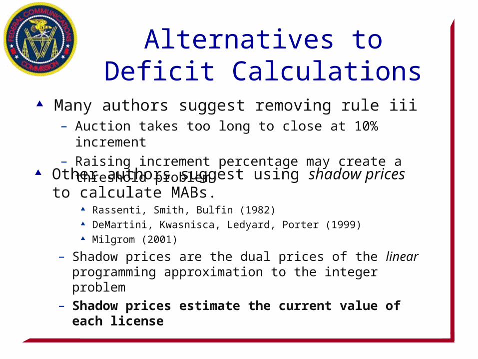
Alternatives to Deficit Calculations

Many authors suggest removing rule iii– Auction takes too long to close at 10% increment

– Raising increment percentage may create a threshold problem

Other authors suggest using shadow prices to calculate MABs.

Rassenti, Smith, Bulfin (1982) DeMartini, Kwasnisca, Ledyard, Porter (1999) Milgrom (2001)

– Shadow prices are the dual prices of the linear programming approximation to the integer problem

– Shadow prices estimate the current value of each license

Alternative Rule iii Shadow Prices

A minimum acceptable bid is the greater of:i. The minimum opening bid

ii. The bidder’s previous high bid on a package plus X%

iii. The estimated value of a package b plus Y%

Note: The estimated value of a package is the sum of the shadow prices of the licenses that make up the package

Bid 2 3 41 5

b3 b4 b5Variables b1 b2,, ,,,,,, = 0 or 1

Maximize $24 b2 $20 b3 $16 b4 $8 b5$22 b1 + + + +

b4License A b1 0 b3 0 <= 1

Count

++++

License B b1 b2 0 b4 0 <= 1++++

b3 0 b5 <=License C 10 b2 ++++

0 0 11 0

Auction FormulationBid

Bid amt.

2

$24

3

$20$22

1 4

$16

5

$8

Package BC ACAB AB C

Objective Value: $30

License A B C

Note: This formulation of the maximum revenue problem ignores the mutual exclusive bid constraints.

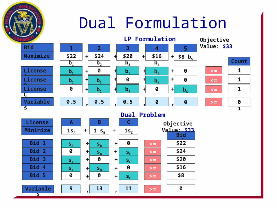
LP Formulation

,, ,,,,,,

Bid 2 3 41 5

b3 b4 b5Variables b1 b2 = 0 or 1

Maximize $24 b2 $20 b3 $16 b4 $8 b5$22 b1 + + + +

b4License A b1

0 b3 0 <= 1

Count

++++License B b1 b2

0 b40 <= 1++++

b3 0 b5 <=License C 10 b2 ++++

0>=b3 b4 b5Variables b1 b2

CBALicense

Variables sA , ,sB sC

1sA 1 sB 1sC

0>=

Bid 1

Bid 2

Bid 3

Bid 4

Bid 5

>=>=>=>=>=

Bid amt.

$22

$24

$20

$16

$8

sA

0

sA

sA

0

sB

sB

0

sB

0

+++

++

0

sC

sC

0

sC

+++

++

Minimize + +

Dual FormulationObjective Value: $33

,, ,,,,,, 0.5 0 00.5 0.5

9 13 11

Objective Value: $33

Dual Problem

Dual prices: Two Problems

Greater than primal

Not unique

Solution: Pseudo-Duals

Rassenti, Smith and Bulfin (1982) as well as DeMartini, Kwasnica, Ledyard and Porter (1999) suggest solving for pseudo-dual prices in order to adjust the over-estimated shadow prices

Use the provisional winners as the “mark” for adjusting down the shadow prices

Result...– The shadow prices sum to equal the revenue obtained from the integer solution

– The sum of the shadow prices of a winning package equals the bid amount of the package

Adjusted Shadow PricesPseudo-Dual Problem

CBALicense

sC

0

sB

sB

0

sB

0

sA

0

sA

sA

0

1sA 1 sB 1sC

Variables sA , ,sB sC0>=

Bid 1

Bid 2

Bid 3

Bid 4

Bid 5

Bid amt.

$22

$24

$20

$16

$8

+

+

+

+

+

0+

+

+

+

+

Minimize + +

sC

sC

>=

>=

>=

>=

>=

3 4Variables 2 ,,,, >= 0

2

3

4

+

+

+

2

3

4

=

=

9 13 8

3 03

Objective Value: $30

valu

e (B

) in

$

value (A) in $

Shadow PriceLicense

A

B

5

5

9

1

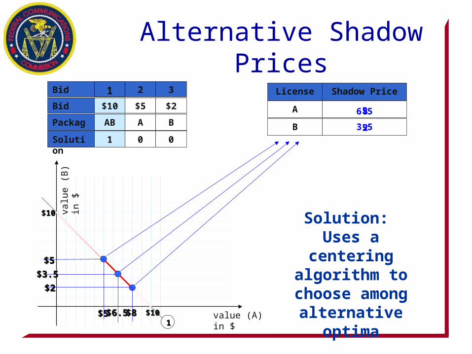
Alternative Shadow Prices

$5$5

$5$5

Bid

Bid amt. $10

1

Package AB

Solution 1

2

8

$9$9

$1$1

11$10$10

$10$10

$2$2

$8$8

valu

e (B

) in

$

value (A) in $

Shadow PriceLicense

A

B

2

$5

A

0

3

$2

B

0

Bid

Bid amt. $10

1

Package AB

Solution 1

11$10$10

$10$10

Bid 2 >=+ $5

BA

Dual Constraints

33$2$2

22

$5$5

Bid 3 >=+ $2

Alternative Shadow Prices

valu

e (B

) in

$

value (A) in $

Shadow PriceLicense

A

B

5

5

6.5

3.5

2

$5

A

0

3

$2

B

0

Bid

Bid amt. $10

1

Package AB

Solution 1

8

2

11$10$10

$10$10

$5$5

$5$5

$2$2

$8$8

$3.5$3.5

$6.5$6.5

Solution: Uses a centering algorithm

to choose among alternative optima

Alternative Shadow Prices

Scaling-up: Testing

Need a method to test the new auction design in larger environments

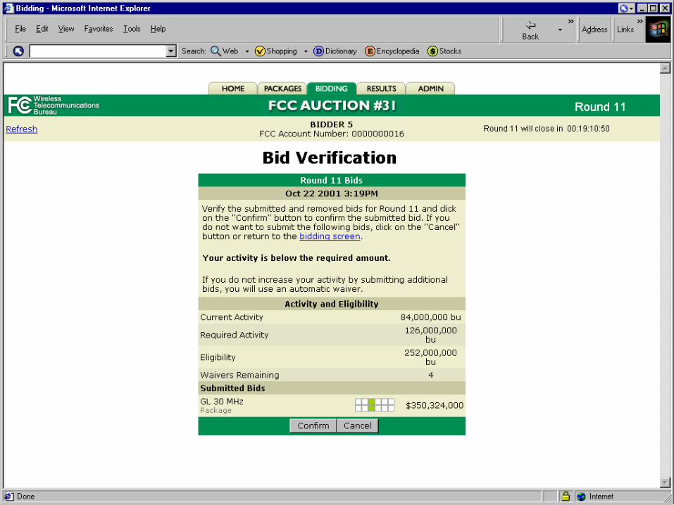
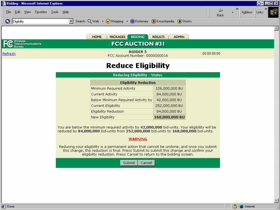
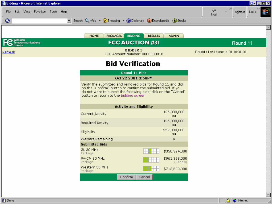
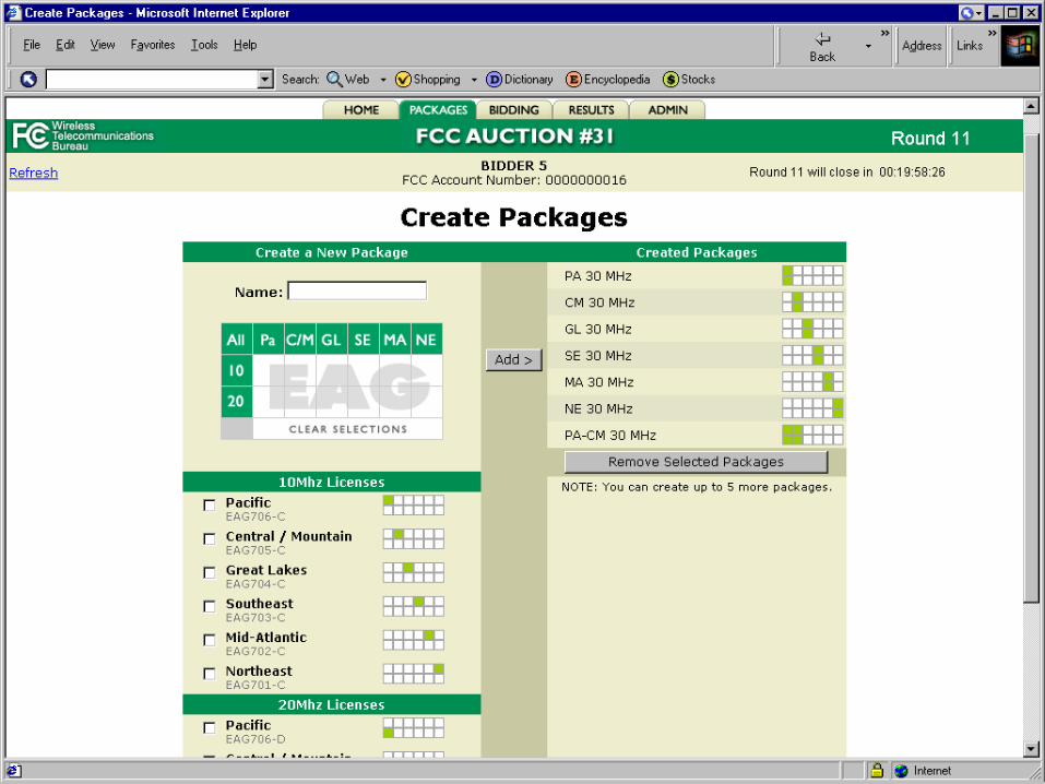
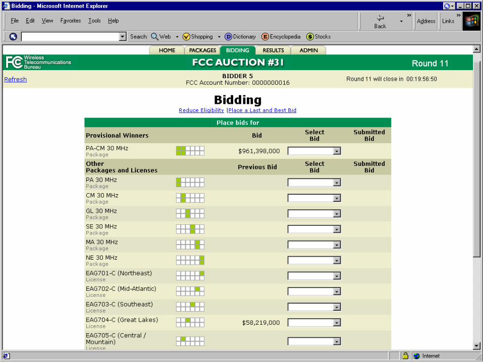
Provides basic bidder functionality– Place new bids (with increments)– Renew previous bids– Dynamically create new packages– Utilize activity waivers– Reduce eligibility

Bidders are given budget constraints Eligibility based on historic data

– Many small bidders with some large bidders Adjacency matrix for geographic synergies that determine the

value of packages Value and straightforward bidders with random increment

bidding based on historical data

BidBot Characteristics

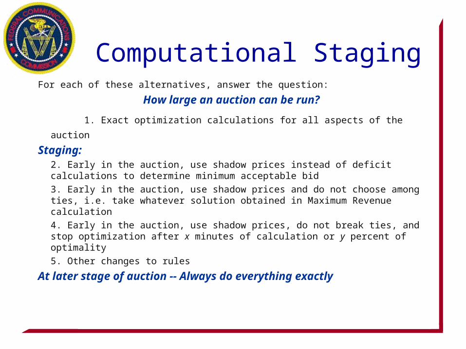
Computational StagingFor each of these alternatives, answer the question:

How large an auction can be run?

1. Exact optimization calculations for all aspects of the auction

Staging: 2. Early in the auction, use shadow prices instead of deficit calculations to

determine minimum acceptable bid

3. Early in the auction, use shadow prices and do not choose among ties, i.e. take whatever solution obtained in Maximum Revenue calculation

4. Early in the auction, use shadow prices, do not break ties, and stop optimization after x minutes of calculation or y percent of optimality

5. Other changes to rules

At later stage of auction -- Always do everything exactly

Where do we go next? More testing using both BidBots and mock auctions Shadow price testing:

– What is the best way to adjust shadow prices?– What happens when licenses have few or no bidders?– How can we obtain a bidder-specific MAB that uses shadow

prices? Click-box bidding versus greater flexibility in submission

of bids:– Does providing more digits of accuracy help to eliminate ties?– Issues of transparency, speed of auction, collusion

When should computational staging occur?

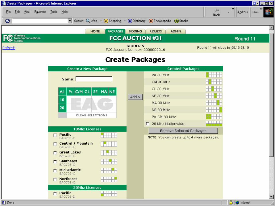
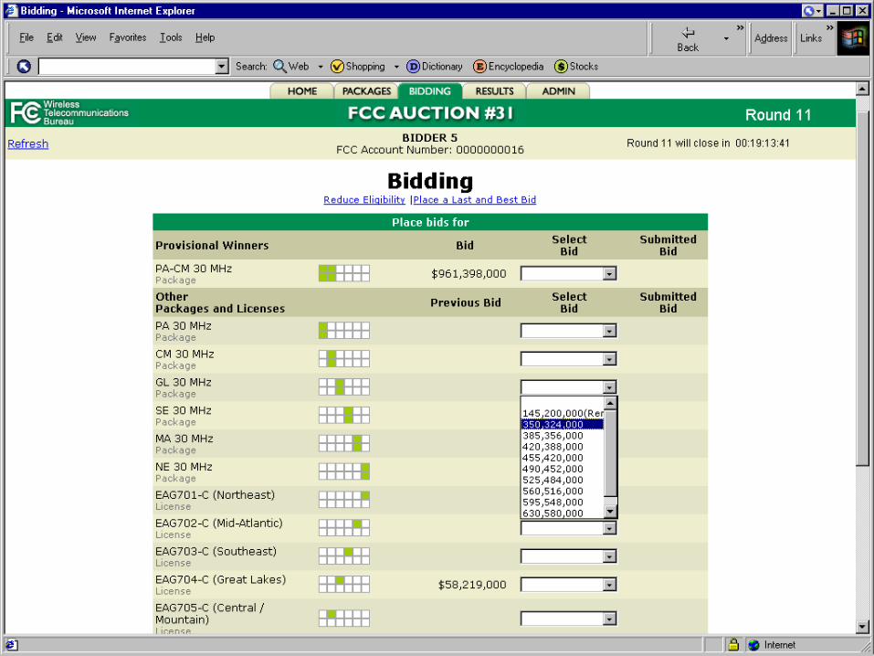
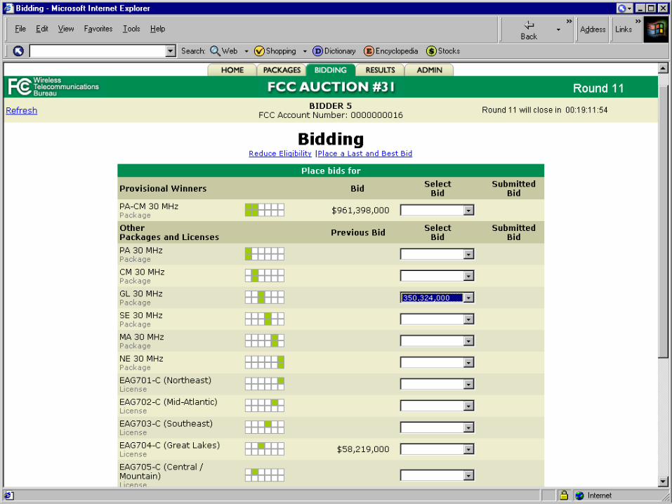
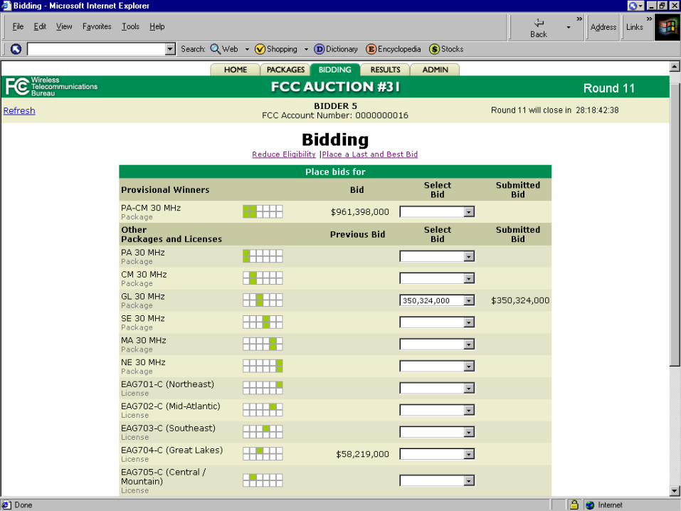
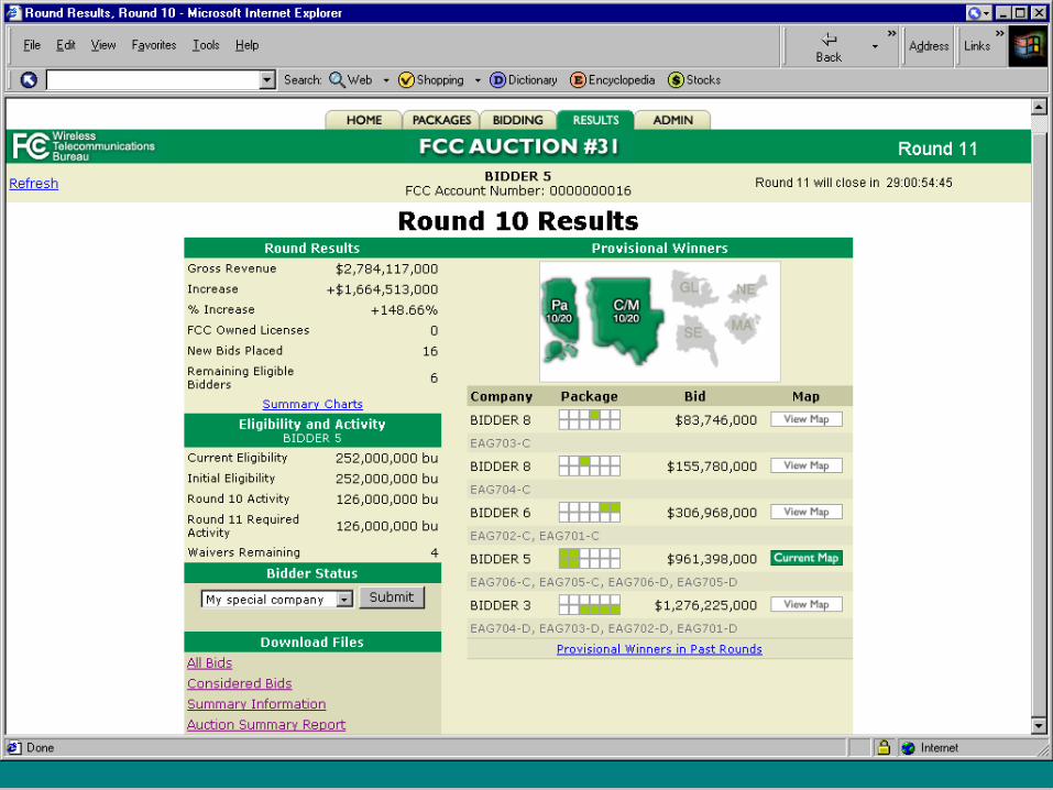
Package Bidding SystemFor Auction 31

Wye River Conference

October 27, 2001

bidder5

*****

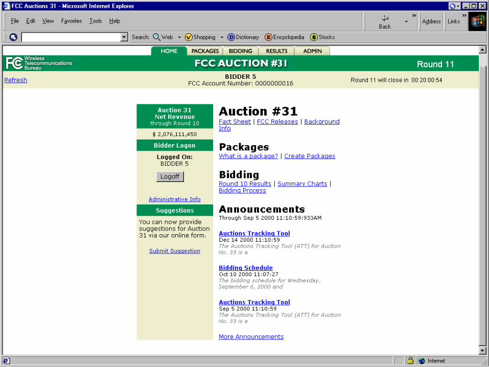
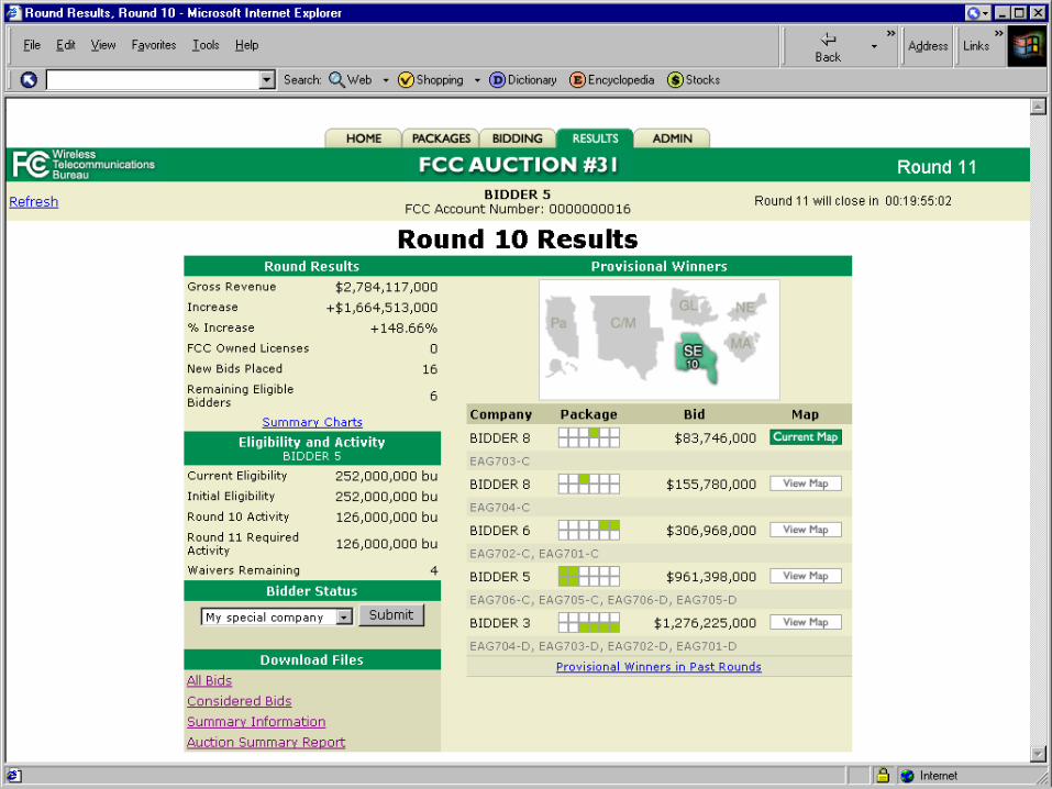
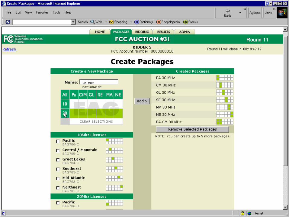
20 MHz nationwide