CS 188 Introduction to Arti cial Intelligence Spring 2021

CS 188 Introduction to Artificial IntelligenceSpring 2021 Note 5

Markov ModelsIn previous notes, we talked about Bayes’ nets and how they are a wonderful structure used for compactlyrepresenting relationships between random variables. We’ll now cover a very intrinsically related structurecalled a Markov model, which for the purposes of this course can be thought of as analogous to a chain-like, infinite-length Bayes’ net. The running example we’ll be working with in this section is the day-to-dayfluctuations in weather patterns. Our weather model will be time-dependent (as are Markov models ingeneral), meaning we’ll have a separate random variable for the weather on each day. If we define Wi as therandom variable representing the weather on day i, the Markov model for our weather example would looklike this:

What information should we store about the random variables involved in our Markov model? To trackhow our quantity under consideration (in this case, the weather) changes over time, we need to know bothit’s initial distribution at time t = 0 and some sort of transition model that characterizes the probabilityof moving from one state to another between timesteps. The initial distribution of a Markov model isenumerated by the probability table given by Pr(W0) and the transition model of transitioning from state i toi+1 is given by Pr(Wi+1|Wi). Note that this transition model implies that the value of Wi+1 is conditionallydependent only on the value of Wi. In other words, the weather at time t = i+ 1 satisfies the Markovproperty or memoryless property, and is independent of the weather at all other timesteps besides t = i.

Using our Markov model for weather, if we wanted to reconstruct the joint between W0, W1, and W2 usingthe chain rule, we would want:

Pr(W0,W1,W2) = Pr(W0)Pr(W1|W0)Pr(W2|W1,W0)

However, with our assumption that the Markov property holds true and W0 |= W2|W1, the joint simplifies to:

Pr(W0,W1,W2) = Pr(W0)Pr(W1|W0)Pr(W2|W1)

And we have everything we need to calculate this from the Markov model. More generally, Markov modelsmake the following independence assumption at each timestep: Wi+1 |= {W0, ...,Wi−1}|Wi. This allows us toreconstruct the joint distribution for the first n+1 variables via the chain rule as follows:

Pr(W0,W1, ...,Wn) = Pr(W0)Pr(W1|W0)Pr(W2|W1)...Pr(Wn|Wn−1) = Pr(W0)n−1

∏i=0

Pr(Wi+1|Wi)

A final assumption that’s typically made in Markov models is that the transition model is stationary. Inother words, for all values of i, Pr(Wi+1|Wi) is identical. This allows us to represent a Markov model withonly two tables: one for Pr(W0) and one for Pr(Wi+1|Wi).

CS 188, Spring 2021, Note 5 1

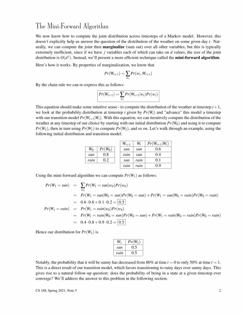
The Mini-Forward AlgorithmWe now know how to compute the joint distribution across timesteps of a Markov model. However, thisdoesn’t explicitly help us answer the question of the distribution of the weather on some given day t. Nat-urally, we can compute the joint then marginalize (sum out) over all other variables, but this is typicallyextremely inefficient, since if we have j variables each of which can take on d values, the size of the jointdistribution is O(d j). Instead, we’ll present a more efficient technique called the mini-forward algorithm.

Here’s how it works. By properties of marginalization, we know that

Pr(Wi+1) = ∑wi

Pr(wi,Wi+1)

By the chain rule we can re-express this as follows:

Pr(Wi+1) = ∑wi

Pr(Wi+1|wi)Pr(wi)

This equation should make some intuitive sense - to compute the distribution of the weather at timestep i+1,we look at the probability distribution at timestep i given by Pr(Wi) and "advance" this model a timestepwith our transition model Pr(Wi+1|Wi). With this equation, we can iteratively compute the distribution of theweather at any timestep of our choice by starting with our initial distribution Pr(W0) and using it to computePr(W1), then in turn using Pr(W1) to compute Pr(W2), and so on. Let’s walk through an example, using thefollowing initial distribution and transition model:

W0 Pr(W0)

sun 0.8rain 0.2

Wi+1 Wi Pr(Wi+1|Wi)

sun sun 0.6rain sun 0.4sun rain 0.1rain rain 0.9

Using the mini-forward algorithm we can compute Pr(W1) as follows:

Pr(W1 = sun) = ∑w0

Pr(W1 = sun|w0)Pr(w0)

= Pr(W1 = sun|W0 = sun)Pr(W0 = sun)+Pr(W1 = sun|W0 = rain)Pr(W0 = rain)

= 0.6 ·0.8+0.1 ·0.2 = 0.5

Pr(W1 = rain) = Pr(W1 = rain|w0)Pr(w0)

= Pr(W1 = rain|W0 = sun)Pr(W0 = sun)+Pr(W1 = rain|W0 = rain)Pr(W0 = rain)

= 0.4 ·0.8+0.9 ·0.2 = 0.5

Hence our distribution for Pr(W1) is

W1 Pr(W1)

sun 0.5rain 0.5

Notably, the probability that it will be sunny has decreased from 80% at time t = 0 to only 50% at time t = 1.This is a direct result of our transition model, which favors transitioning to rainy days over sunny days. Thisgives rise to a natural follow-up question: does the probability of being in a state at a given timestep everconverge? We’ll address the answer to this problem in the following section.


Stationary DistributionTo solve the problem stated above, we must compute the stationary distribution of the weather. As thename suggests, the stationary distribution is one that remains the same after the passage of time, i.e.

Pr(Wt+1) = Pr(Wt)

We can compute these converged probabilities of being in a given state by combining the above equivalencewith the same equation used by the mini-forward algorithm:

Pr(Wt+1) = Pr(Wt) = ∑wt

Pr(Wt+1|wt)Pr(wt)

For our weather example, this gives us the following two equations:

Pr(Wt = sun) = Pr(Wt+1 = sun|Wt = sun)Pr(Wt = sun)+Pr(Wt+1 = sun|Wt = rain)Pr(Wt = rain)

= 0.6 ·Pr(Wt = sun)+0.1 ·Pr(Wt = rain)

Pr(Wt = rain) = Pr(Wt+1 = rain|Wt = sun)Pr(Wt = sun)+Pr(Wt+1 = rain|Wt = rain)Pr(Wt = rain)

= 0.4 ·Pr(Wt = sun)+0.9 ·Pr(Wt = rain)

We now have exactly what we need to solve for the stationary distribution, a system of 2 equations in 2unknowns! We can get a third equation by using the fact that Pr(Wt) is a probability distribution and somust sum to 1:

Pr(Wt = sun) = 0.6 ·Pr(Wt = sun)+0.1 ·Pr(Wt = rain)

Pr(Wt = rain) = 0.4 ·Pr(Wt = sun)+0.9 ·Pr(Wt = rain)

1 = Pr(Wt = sun)+Pr(Wt = rain)

Solving this system of equations yields Pr(Wt = sun) = 0.2 and Pr(Wt = rain) = 0.8. Hence the table forour stationary distribution, which we’ll henceforth denote as Pr(W∞), is the following:

W∞ Pr(W∞)

sun 0.2rain 0.8

To verify this result, let’s apply the transition model to the stationary distribution:

Pr(W∞+1 = sun) = Pr(W∞+1 = sun|W∞ = sun)Pr(W∞ = sun)+Pr(W∞+1 = sun|W∞ = rain)Pr(W∞ = rain)

= 0.6 ·0.2+0.1 ·0.8 = 0.2

Pr(W∞+1 = rain) = Pr(W∞+1 = rain|W∞ = sun)Pr(W∞ = sun)+Pr(W∞+1 = rain|W∞ = rain)Pr(W∞ = rain)

= 0.4 ·0.2+0.9 ·0.8 = 0.8

As expected, Pr(W∞+1) = Pr(W∞). In general, if Wt had a domain of size k, the equivalence

Pr(Wt) = ∑wt

Pr(Wt+1|wt)Pr(wt)

yields a system of k equations, which we can use to solve for the stationary distribution.


Hidden Markov ModelsWith Markov models, we saw how we could incorporate change over time through a chain of random vari-ables. For example, if we want to know the weather on day 10 with our standard Markov model from above,we can begin with the initial distribution Pr(W0) and use the mini-forward algorithm with our transitionmodel to compute Pr(W10). However, between time t = 0 and time t = 10, we may collect new meteoro-logical evidence that might affect our belief of the probability distribution over the weather at any giventimestep. In simpler terms, if the weather forecasts an 80% chance of rain on day 10, but there are clearskies on the night of day 9, that 80% probability might drop drastically. This is exactly what the HiddenMarkov Model helps us with - it allows us to observe some evidence at each timestep, which can potentiallyaffect the belief distribution at each of the states. The Hidden Markov Model for our weather model can bedescribed using a Bayes’ net structure that looks like the following:

Unlike vanilla Markov models, we now have two different types of nodes. To make this distinction, we’ll calleach Wi a state variable and each weather forecast Fi an evidence variable which in the lecture we denotedwith Ei. Since Wi encodes our belief of the probability distribution for the weather on day i, it should bea natural result that the weather forecast for day i is conditionally dependent upon this belief. The modelimplies similar conditional indepencence relationships as standard Markov models, with an additional set ofrelationships for the evidence variables:

F1 |= W0|W1

∀i = 2, . . . ,n; Wi |= {W0, . . . ,Wi−2,F1, . . . ,Fi−1}|Wi−1

∀i = 2, . . . ,n; Fi |= {W0, . . . ,Wi−1,F1, . . . ,Fi−1}|Wi

Just like Markov models, Hidden Markov Models make the assumption that the transition model Pr(Wi+1|Wi)is stationary. Hidden Markov Models make the additional simplifying assumption that the sensor modelPr(Fi|Wi) is stationary as well. Hence any Hidden Markov Model can be represented compactly with justthree probability tables: the initial distribution, the transition model, and the sensor model.

We’ll define the belief distribution at time i with all evidence F1, . . . ,Fi observed up to date:

Pr(Wi| f1, . . . , fi)

Similarly, we’ll define as the belief distribution at time i with evidence f1, . . . , fi−1 observed:

Pr(Wi| f1, . . . , fi−1)

Notation-wise you might sometimes see the aggregated evidence from timesteps 1 ≤ i ≤ t re-expressed inthe following form:

e1:t = e1, . . . ,et

Under this notation, Pr(Wi| f1, . . . , fi−1) can be written as Pr(Wi| f1:(i−1)). This notation will become relevantin the upcoming sections, where we’ll discuss time elapse updates that iteratively incorporate new evidenceinto our weather model.


The Forward AlgorithmUsing the conditional probability assumptions stated above and marginalization properties of conditionalprobability tables, we can derive a relationship between Pr(Wi| f1, . . . , fi) and Pr(Wi| f1, . . . , fi−1) that’s ofthe same form as the update rule for the mini-forward algorithm. We begin by using marginalization:

Pr(Wi+1| f1, . . . , fi) = ∑wi

Pr(Wi+1,wi| f1, . . . , fi)

This can be re-expressed then with the chain rule as follows:

Pr(Wi+1| f1, . . . , fi) = ∑wi

Pr(Wi+1|wi, f1, . . . , fi)Pr(wi| f1, . . . , fi)

Given that Wi+1 |= { f1, . . . fi}|Wi, this implies to our final relationship that:

Pr(Wi+1| f1, . . . , fi) = ∑wi

Pr(Wi+1|wi)Pr(wi| f1, . . . , fi)

Now let’s consider how we can derive a relationship between Pr(Wi+1| f1, . . . , fi) and Pr(Wi+1| f1, . . . , fi+1).By simple application of Bayes’ rule, we can see that

Pr(Wi+1| f1, . . . , fi+1) =Pr(Wi+1, fi+1| f1, . . . , fi)

Pr( fi+1| f1, . . . , fi)

When dealing with conditional probabilities a commonly used trick is to delay normalization until we requirethe normalized probabilities, a trick we’ll now employ. More specifically, since the denominator in theabove expansion is common to every term in the probability table represented by Pr(Wi+1| f1, . . . , fi+1), wecan omit actually dividing by Pr( fi+1| f1, . . . , fi). Instead, we can simply note that Pr(Wi+1| f1, . . . , fi+1) isproportional to Pr(Wi+1, fi+1| f1, . . . , fi) which we denote as:

Pr(Wi+1| f1, . . . , fi+1) ∝ Pr(Wi+1, fi+1| f1, . . . , fi)

with a constant of proportionality equal to Pr( fi+1| f1, . . . , fi). The notation above is equivalent to sayingPr(Wi+1| f1, . . . , fi+1) = αPr(Wi+1, fi+1| f1, . . . , fi). Whenever we decide we want to recover the belief dis-tribution Pr(Wi+1| f1, . . . , fi+1), we can divide each computed value by this constant of proportionality. Now,using the chain rule we can observe the following:

Pr(Wi+1| f1, . . . , fi+1) ∝ Pr(Wi+1, fi+1| f1, . . . , fi) = Pr( fi+1|Wi+1, f1, . . . , fi)Pr(Wi+1| f1, . . . , fi)

By the conditional independence assumptions associated with Hidden Markov Models stated previously,Pr( fi+1|Wi+1, f1, . . . , fi) is equivalent to simply Pr( fi+1|Wi+1). This allows us to express the relationshipbetween Pr(Wi+1| f1, . . . , fi) and Pr(Wi+1| f1, . . . , fi+1) in it’s final form:

Pr(Wi+1| f1, . . . , fi+1) ∝ Pr( fi+1|Wi+1)Pr(Wi+1| f1, . . . , fi)

Combining the two relationships we’ve just derived an iterative algorithm known as the forward algorithm,the Hidden Markov Model analog of the mini-forward algorithm from earlier:

Pr(Wi+1| f1, . . . , fi+1) ∝ Pr( fi+1|Wi+1)∑wi

Pr(Wi+1|wi)Pr(wi| f1, . . . , fi)


The forward algorithm can be thought of as consisting of two distinctive steps: the time elapse update whichcorresponds to determining Pr(Wi+1| f1, . . . , fi) from Pr(Wi| f1, . . . , fi) and the observation update whichcorresponds to determining Pr(Wi+1| f1, . . . , fi+1) from Pr(Wi+1| f1, . . . , fi). Hence, in order to advance ourbelief distribution by one timestep (i.e. compute Pr(Wi+1| f1, . . . , fi+1 from Pr(Wi| f1, . . . , fi), we must firstadvance our model’s state by one timestep with the time elapse update, then incorporate new evidence fromthat timestep with the observation update. Consider the following initial distribution, transition model, andsensor model:

W0 P(W0)

sun 0.8rain 0.2

Wi+1 Wi Pr(Wi+1|Wi)

sun sun 0.6rain sun 0.4sun rain 0.1rain rain 0.9

Fi Wi Pr(Fi|Wi)

good sun 0.8bad sun 0.2

good rain 0.3bad rain 0.7

To compute Pr(W1), we begin by performing a time update to get:

Pr(W1 = sun) = ∑w0

Pr(W1 = sun|w0)Pr(w0)

= Pr(W1 = sun|W0 = sun)Pr(W0 = sun)+Pr(W1 = sun|W0 = rain)Pr(W0 = rain)

= 0.6 ·0.8+0.1 ·0.2 = 0.5

Pr(W1 = rain) = ∑w0

Pr(W1 = rain|w0)Pr(w0)

= Pr(W1 = rain|W0 = sun)Pr(W0 = sun)+Pr(W1 = rain|W0 = rain)Pr(W0 = rain)

= 0.4 ·0.8+0.9 ·0.2 = 0.5

Hence:

W1 P(W1)

sun 0.5rain 0.5

Next, we’ll assume that the weather forecast for day 1 was good (i.e. F1 = good), and perform an observationupdate to get Pr(W1|F1):

Pr(W1 = sun|F1 = good) ∝ Pr(F1 = good|W1 = sun)Pr(W1 = sun) = 0.8 ·0.5 = 0.4

Pr(W1 = rain|F1 = good) ∝ Pr(F1 = good|W1 = rain)Pr(W1 = rain) = 0.3 ·0.5 = 0.15

The last step is to normalize P(W1|F1), noting that the entries in table for P(W1|F1) sum to 0.4+0.15 = 0.55:

Pr(W1 = sun|F1 = good) = 0.4/0.55 =811

Pr(W1 = rain|F1 = good) = 0.15/0.55 =311

Our final table for P(W1|F1) is thus the following:

W1 P(W1|F1)

sun 8/11rain 3/11


Note the result of observing the weather forecast. Because the weatherman predicted good weather, ourbelief that it would be sunny increased from 1

2 after the time update to 811 after the observation update.

As a parting note, the normalization trick discussed above can actually simplify computation significantlywhen working with Hidden Markov Models. If we began with some initial distribution and were interestedin computing the belief distribution at time t, we could use the forward algorithm to iteratively compute thebeliefs at time steps 1, . . . , t and normalize only once at the end.

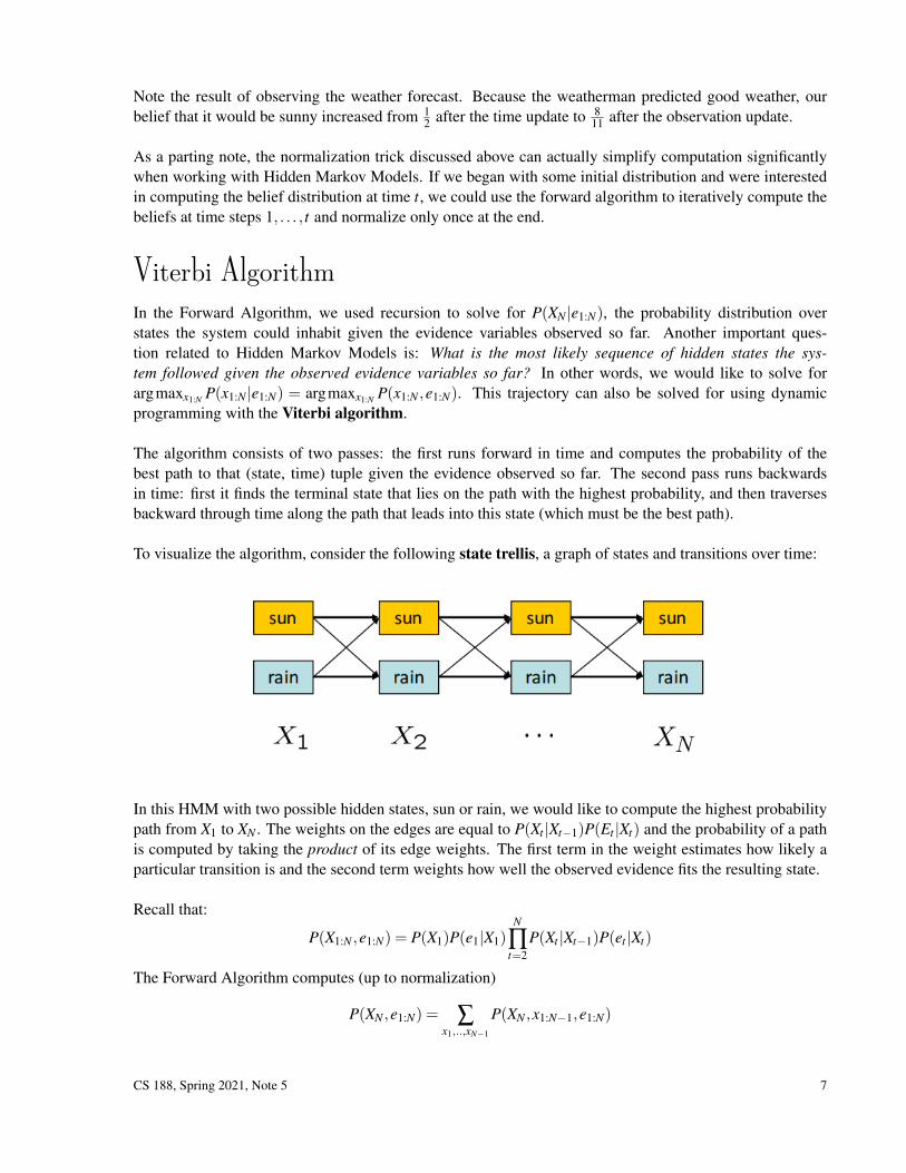
Viterbi AlgorithmIn the Forward Algorithm, we used recursion to solve for P(XN |e1:N), the probability distribution overstates the system could inhabit given the evidence variables observed so far. Another important ques-tion related to Hidden Markov Models is: What is the most likely sequence of hidden states the sys-tem followed given the observed evidence variables so far? In other words, we would like to solve forargmaxx1:N P(x1:N |e1:N) = argmaxx1:N P(x1:N ,e1:N). This trajectory can also be solved for using dynamicprogramming with the Viterbi algorithm.

The algorithm consists of two passes: the first runs forward in time and computes the probability of thebest path to that (state, time) tuple given the evidence observed so far. The second pass runs backwardsin time: first it finds the terminal state that lies on the path with the highest probability, and then traversesbackward through time along the path that leads into this state (which must be the best path).

To visualize the algorithm, consider the following state trellis, a graph of states and transitions over time:

In this HMM with two possible hidden states, sun or rain, we would like to compute the highest probabilitypath from X1 to XN . The weights on the edges are equal to P(Xt |Xt−1)P(Et |Xt) and the probability of a pathis computed by taking the product of its edge weights. The first term in the weight estimates how likely aparticular transition is and the second term weights how well the observed evidence fits the resulting state.

Recall that:

P(X1:N ,e1:N) = P(X1)P(e1|X1)N

∏t=2

P(Xt |Xt−1)P(et |Xt)

The Forward Algorithm computes (up to normalization)

P(XN ,e1:N) = ∑x1,..,xN−1

P(XN ,x1:N−1,e1:N)


In the Viberbi Algorithm, we want to compute

arg maxx1,..,xN

P(x1:N ,e1:N)

to find the maximum likelihood estimate of the sequence of hidden states. Notice that each term in the prod-uct is exactly the expression for the edge weight between layer t− 1 to layer t. So, the product of weightsalong the path on the trellis gives us the probability of the path given the evidence.

We could solve for a joint probability table over all of the possible hidden states, but this results in anexponential space cost. Given such a table, we could use dynamic programming to compute the best path inpolynomial time. However, because we can use dynamic programming to compute the best path, we don’tnecessarily need the whole table at any given time.

Define mt [xt ] = maxx1:t−1 P(x1:t ,e1:t), or the maximum probability of a path starting at any x0 and the ev-idence seen so far to a given xt at time t. This is the same as the highest weight path through the trellis fromstep 1 to t. Also note that

mt [xt ] = maxx1:t−1

P(et |xt)P(xt |xt−1)P(x1:t−1,e1:t−1) (1)

= P(et |xt)maxxt−1

P(xt |xt−1)maxx1:t−2

P(x1:t−1,e1:t−1) (2)

= P(et |xt)maxxt−1

P(xt |xt−1)mt−1[xt−1]. (3)

This suggests that we can compute mt for all t recursively via dynamic programming. This makes it possibleto determine the last state xN for the most likely path, but we still need a way to backtrack to reconstruct theentire path. Let’s define at [xt ] = P(et |xt)argmaxxt−1 P(xt |xt−1)mt−1[xt−1] = argmaxxt−1 P(xt |xt−1)mt−1[xt−1]to keep track of the last transition along the best path to xt . We can now outline the algorithm.

Result: Most likely sequence of hidden states x∗1:N/* Forward pass */for t = 1 to N do

for xt ∈X doif t = 1 then

mt [xt ] = P(xt)P(e0|xt)else

at [xt ] = argmaxxt−1 P(xt |xt−1)mt−1[xt−1];mt [xt ] = P(et |xt)P(xt |at [xt ])mt−1[at [xt ]];

endend

end/* Find the most likely path’s ending point */x∗N = argmaxxN mN [xN ];/* Work backwards through our most likely path and find the hidden

states */for t = N to 2 do

x∗t−1 = at [x∗t ];end

Notice that our a arrays define a set of N sequences, each of which is the most likely sequence to a particularend state xN . Once we finish the forward pass, we look at the likelihood of the N sequences, pick the best


one, and reconstruct it in the backwards pass. We have thus computed the most likely explanation for ourevidence in polynomial space and time.

Particle FilteringRecall that with Bayes’ nets, when running exact inference was too computationally expensive, using one ofthe sampling techniques we discussed was a viable alternative to efficiently approximate the desired proba-bility distribution(s) we wanted. Hidden Markov Models have the same drawback - the time it takes to runexact inference with the forward algorithm scales with the number of values in the domains of the randomvariables. This was acceptable in our current weather problem formulation where the weather can only takeon 2 values, Wi ∈ {sun,rain}, but say instead we wanted to run inference to compute the distribution ofthe actual temperature on a given day to the nearest tenth of a degree. The Hidden Markov Model analogto Bayes’ net sampling is called particle filtering, and involves simulating the motion of a set of particlesthrough a state graph to approximate the probability (belief) distribution of the random variable in question.

Instead of storing a full probability table mapping each state to its belief probability, we’ll instead store alist of n particles, where each particle is in one of the d possible states in the domain of our time-dependentrandom variable. Typically, n is significantly smaller than d (denoted symbolically as n << d) but still largeenough to yield meaningful approximations; otherwise the performance advantage of particle filtering be-comes negligible. Our belief that a particle is in any given state at any given timestep is dependent entirelyon the number of particles in that state at that timestep in our simulation. For example, say we indeed wantedto simulate the belief distribution of the temperature T on some day i and assume for simplicity that thistemperature can only take on integer values in the range [10,20] (d = 11 possible states). Assume furtherthat we have n = 10 particles, which take on the following values at timestep i of our simulation:

[15,12,12,10,18,14,12,11,11,10]

By taking counts of each temperature that appears in our particle list and diving by the total number ofparticles, we can generate our desired empirical distribution for the temperature at time i:

Ti 10 11 12 13 14 15 16 17 18 19 20B(Ti) 0.2 0.2 0.3 0 0.1 0.1 0 0 0.1 0 0

Now that we’ve seen how to recover a belief distribution from a particle list, all that remains to be discussedis how to generate such a list for a timestep of our choosing.

Particle Filtering SimulationParticle filtering simulation begins with particle initialization, which can be done quite flexibly - we cansample particles randomly, uniformly, or from some initial distribution. Once we’ve sampled an initial listof particles, the simulation takes on a similar form to the forward algorithm, with a time elapse updatefollowed by an observation update at each timestep:

• Time Elapse Update - Update the value of each particle according to the transition model. For aparticle in state ti, sample the updated value from the probability distribution given by Pr(Ti+1|ti).Note the similarity of the time elapse update to prior sampling with Bayes’ nets, since the frequencyof particles in any given state reflects the transition probabilities.


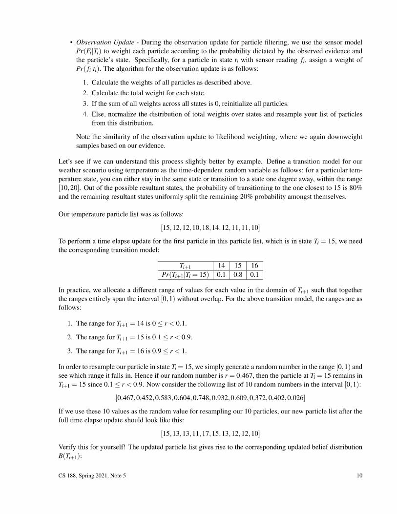
• Observation Update - During the observation update for particle filtering, we use the sensor modelPr(Fi|Ti) to weight each particle according to the probability dictated by the observed evidence andthe particle’s state. Specifically, for a particle in state ti with sensor reading fi, assign a weight ofPr( fi|ti). The algorithm for the observation update is as follows:

1. Calculate the weights of all particles as described above.2. Calculate the total weight for each state.3. If the sum of all weights across all states is 0, reinitialize all particles.4. Else, normalize the distribution of total weights over states and resample your list of particles

from this distribution.

Note the similarity of the observation update to likelihood weighting, where we again downweightsamples based on our evidence.

Let’s see if we can understand this process slightly better by example. Define a transition model for ourweather scenario using temperature as the time-dependent random variable as follows: for a particular tem-perature state, you can either stay in the same state or transition to a state one degree away, within the range[10,20]. Out of the possible resultant states, the probability of transitioning to the one closest to 15 is 80%and the remaining resultant states uniformly split the remaining 20% probability amongst themselves.

Our temperature particle list was as follows:

[15,12,12,10,18,14,12,11,11,10]

To perform a time elapse update for the first particle in this particle list, which is in state Ti = 15, we needthe corresponding transition model:

Ti+1 14 15 16Pr(Ti+1|Ti = 15) 0.1 0.8 0.1

In practice, we allocate a different range of values for each value in the domain of Ti+1 such that togetherthe ranges entirely span the interval [0,1) without overlap. For the above transition model, the ranges are asfollows:

1. The range for Ti+1 = 14 is 0≤ r < 0.1.

2. The range for Ti+1 = 15 is 0.1≤ r < 0.9.

3. The range for Ti+1 = 16 is 0.9≤ r < 1.

In order to resample our particle in state Ti = 15, we simply generate a random number in the range [0,1) andsee which range it falls in. Hence if our random number is r = 0.467, then the particle at Ti = 15 remains inTi+1 = 15 since 0.1≤ r < 0.9. Now consider the following list of 10 random numbers in the interval [0,1):

[0.467,0.452,0.583,0.604,0.748,0.932,0.609,0.372,0.402,0.026]

If we use these 10 values as the random value for resampling our 10 particles, our new particle list after thefull time elapse update should look like this:

[15,13,13,11,17,15,13,12,12,10]

Verify this for yourself! The updated particle list gives rise to the corresponding updated belief distributionB(Ti+1):


Ti 10 11 12 13 14 15 16 17 18 19 20B(Ti+1) 0.1 0.1 0.2 0.3 0 0.2 0 0.1 0 0 0

Comparing our updated belief distribution B(Ti+1) to our initial belief distribution B(Ti), we can see that asa general trend the particles tend to converge towards a temperature of T = 15.

Next, let’s perform the observation update, assuming that our sensor model Pr(Fi|Ti) states that the prob-ability of a correct forecast fi = ti is 80%, with a uniform 2% chance of the forecast predicting any of theother 10 states. Assuming a forecast of Fi+1 = 13, the weights of our 10 particles are as follows:

Particle p1 p2 p3 p4 p5 p6 p7 p8 p9 p10

State 15 13 13 11 17 15 13 12 12 10Weight 0.02 0.8 0.8 0.02 0.02 0.02 0.8 0.02 0.02 0.02

Then we aggregate weights by state:

State 10 11 12 13 15 17Weight 0.02 0.02 0.04 2.4 0.04 0.02

Summing the values of all weights yields a sum of 2.54, and we can normalize our table of weights togenerate a probability distribution by dividing each entry by this sum:

State 10 11 12 13 15 17Weight 0.02 0.02 0.04 2.4 0.04 0.02

Normalized Weight 0.0079 0.0079 0.0157 0.9449 0.0157 0.0079

The final step is to resample from this probability distribution, using the same technique we used to resam-ple during the time elapse update. Let’s say we generate 10 random numbers in the range [0,1) with thefollowing values:

[0.315,0.829,0.304,0.368,0.459,0.891,0.282,0.980,0.898,0.341]

This yields a resampled particle list as follows:

[13,13,13,13,13,13,13,15,13,13]

With the corresponding final new belief distribution:

Ti 10 11 12 13 14 15 16 17 18 19 20B(Ti+1) 0 0 0 0.9 0 0.1 0 0 0 0 0

Observe that our sensor model encodes that our weather prediction is very accurate with probability 80%,and that our new particles list is consistent with this since most particles are resampled to be Ti+1 = 13.


SummaryIn this note, we covered two new types of models:

• Markov models, which encode time-dependent random variables that possess the Markov property.We can compute a belief distribution at any timestep of our choice for a Markov model using proba-bilistic inference with the mini-forward algorithm.

• Hidden Markov Models, which are Markov models with the additional property that new evidencewhich can affect our belief distribution can be observed at each timestep. To compute the beliefdistribution at any given timestep with Hidden Markov Models, we use the forward algorithm.

Sometimes, running exact inference on these models can be too computationally expensive, in which casewe can use particle filtering as a method of approximate inference.


Documents

CS 188 Introduction to Arti cial Intelligence Spring 2021