CS 188 Arti cial Intelligence Final - Amazon S3 · Arti cial Intelligence Final You have approximately 3 hours. The exam is closed book, closed notes except your three one-page crib

CS 188Fall 2012

Introduction toArtificial Intelligence Final

� You have approximately 3 hours.

� The exam is closed book, closed notes except your three one-page crib sheets.

� Please use non-programmable calculators only.

� Mark your answers ON THE EXAM ITSELF. If you are not sure of your answer you may wish to provide abrief explanation. All short answer sections can be successfully answered in a few sentences AT MOST.

First name

Last name

SID

First and last name of student to your left

First and last name of student to your right

For staff use only:Q1. Warm-Up /1Q2. Search: Return of the Slugs /10Q3. CSPs: Enforcing Arc Consistency /6Q4. CSPs and Bayes’ Nets /10Q5. Games: 3-Player Pruning /18Q6. Reinforcement Learning /6Q7. Bandits /22Q8. Bayes’ Nets Representation /12Q9. Preprocessing Bayes’ Net Graphs for Inference /11Q10. Clustering /8Q11. Decision Trees /6Q12. Machine Learning: Overfitting /10

Total /120

1

THIS PAGE IS INTENTIONALLY LEFT BLANK

Q1. [1 pt] Warm-Up

Circle the CS188 mascot

3

Q2. [10 pts] Search: Return of the SlugsAs shown in the diagram on the left, two slugs A and B want to exit a maze via exits E1 and E2. At each timestep, each slug can either stay in place or move to an adjacent free square. A slug cannot move into a square thatthe other slug is moving into. Either slug may use either exit, but they cannot both use the same exit. When a slugmoves, it leaves behind a poisonous substance. The substance remains in the square for 2 time steps; during thistime, no slug can move into the poisonous square.

For example, if slugs A and B begin in the positions shown above on the left, and slug A moves Down 3 steps whileslug B moves Right three steps, then the world becomes as shown above on the right, with ×’s marking the poisonoussquares. Note that slug A does have the option of moving Right from its current position, since the trail from B willevaporate by the time it arrives.

You must pose a search problem that will get both slugs to the exits in as few time steps as possible. Assume thatthe board is of size M by N . While all answers should hold for a general board, not just the one shown above, youdo not need to generalize beyond two slugs, two exits, or two timesteps of decay for the slug trails.

(a) [4 pts] How many states are there in a minimal representation of the space? Justify with a brief description ofthe components of your state space. (MN)2 · 52

Our state space needs to encode the position of each slug (MN possibilities per slug, so (MN)2 for both slugs)as well as the slug trails. Note that we only need to track the more recent of the two squares in each trail,since the second square will evaporate before the next move and so has no effect on the available actions (thisis a subtle point, so we still gave full credit to solutions which tracked both squares). Given a slug’s location,there are five possible locations for its trail (immediately North, East, South, West of the slug, or directlyunderneath the slug if its most recent action was to stay in place), so there are 52 possibilities for the trails ofthe two slugs. Note that this representation is significantly more efficient than if we had specified the explicitcoordinates of each trail.

(b) [6 pts] Let d(x, y) denote Manhattan distance between x and and y. Consider three heuristics, defined in termsof slug locations A and B and exit locations E1 and E2. Remember that either slug can use either exit, butthey must use different exits.

Definition Explanationh1 = max

s∈{A,B}min(d(s, E1), d(s, E2)) Return the maximum, over the two slugs, of the distance from the

slug to its closest exit.h2 = max (d(A,E1), d(B,E2)) Assign slug A to exit E1 and B to E2; then return the maximum

distance from either slug to its assigned exit.h3 = min

(e,e′)∈{(E1,E2),(E2,E1)}max(d(A, e), d(B, e′)) Return the max distance from a slug to its assigned exit, under the

assignment of slugs to distinct exits which minimizes this quantity.

(i) [3 pts] Which of these three heuristics are admissible? Fill in all that apply.

h1 © h2 h3

(ii) [3 pts] For each pair of heuristics, fill in the circle which correctly describes their dominance relationship.Note: dominance is defined regardless of admissibility.

© h1 dominates h2 h2 dominates h1 © h1 = h2 © none

© h1 dominates h3 h3 dominates h1 © h1 = h3 © none

h2 dominates h3 © h3 dominates h2 © h2 = h3 © none

4

Q3. [6 pts] CSPs: Enforcing Arc ConsistencyYou are given a CSP with three variables: A, B, and C. Each variable has an initial domain of {1, 2, 3}. Thefollowing constraints apply:

� A 6= B

� A 6= C

� B > C

(a) [4 pts] Arcs: You are asked to enforce arc-consistency in this CSP. Assume that the algorithm for enforcingarc consistency initially starts with all arcs in a queue in alphabetical order (as below). The queue is thereafterprocessed in a first-in-first-out manner, so any new arcs are processed in the order they are added.

Fill in the circles for any arcs that are re-inserted into the queue at some point. Note: if an arc is already inthe queue, it cannot be “added” to the queue.

© A→ BX

© A→ CX

© B → A

© B → CX

© C → A

© C → B

A must be re-checked after the domain of B or C is reduced and B must be checked after the domain of C isreduced (when enforcing C → B).

(b) [2 pts] Domains: Cross off the values that are eliminated from each variable’s domain below:

A 1 2 3

B 2 3

C 1 2

5

Q4. [10 pts] CSPs and Bayes’ NetsWe consider how to solve CSPs by converting them to Bayes’ nets.

(a) A Simple CSP

First, assume that you are given a CSP over two binary variables, A and B, with only one constraint: A 6= B.

As shown below, the Bayes’ net is composed of nodes A and B, and an additional node for a binary randomvariable O1 that represents the constraint. O1 = +o1 when A and B satisfy the constraint, and O1 = −o1when they do not. The way you will solve for values of A and B that satisfy the CSP is by running inferencefor the query P (A,B | +o1). The setting(s) of A,B with the highest probability will satisfy the constraints.

(i) [2 pts] Fill in the values in the rightmost CPT that will allow you to perform the inference queryP (A,B | +o1) with correct results.

O1

BA

A P (A)−a 0.5+a 0.5

B P (B)−b 0.5+b 0.5

A B O1 P (O1 | A,B)−a −b −o1 1−a −b +o1 0−a +b −o1 0−a +b +o1 1+a −b −o1 0+a −b +o1 1+a +b −o1 1+a +b +o1 0

+o1 is an indicator for a 6= b and −o1 is an indicator for the complement a = b.

(ii) [2 pts] Compute the Posterior Distribution: Now you can find the solution(s) using probabilisticinference. Fill in the values below. Refer to the table in pt. (i).

O1 A B P (A,B | +o1)+o1 −a −b 0+o1 −a +b 1/2+o1 +a −b 1/2+o1 +a +b 0

(b) [3 pts] A More Complex CSP

The graph below on the left shows a more complex CSP, over variables A, B, C, D. Recall that nodes in thisgraph correspond to variables that can be assigned values, and an edge between two nodes corresponds to aconstraint that involves both of the variables.

To the right of the graph below, draw the Bayes’ Net that, when queried for the posterior P (A,B,C,D |+o1,+o2,+o3), will assign the highest probability to the setting(s) of values that satisfy all constraints. Youdo not need to specify any of the CPTs. Permuting o1, o2, o3 is acceptable since the variable-constraint cor-resondence was not given.

C

BA

D

6

(c) [3 pts] Unsatisfiable Constraints

It may be the case that there is no solution that satisfies all constraints of a CSP. We decide to deal with thisby adding an extra set of variables to our Bayes’ Net representation of the CSP: for each constraint variableOi, we add a child binary random variable Ni for constraint satisfaction, and condition on +ni instead of on+oi.

For example, the Bayes’ Net for the two-variable CSP from before will look like thegraph on the right. Furthermore, we con-struct the new CPT to have the form of theCPT on the right.

O1

BA

N1

O1 N1 P (N1 | O1)−o1 −n1 p−o1 +n1 1− p+o1 −n1 q+o1 +n1 1− q

Consider a CSP over three binary variables A, B, C with the constraints that no two variableshave the same value.

Write an expression below in terms of p and/or q, and standard mathematical operators (e.g. pq < 0.1 orp = q), that will guarantee that solutions satisfying more constraints have higher posterior probabilityP (A,B,C | +n1,+n2,+n3). Keep in mind that not all constraints can be satisfied at the same time.

Your expression:

We want a satisfying setting of the parents of o to be more likely than an unsatisfying setting of the parentsof o. We also know that n is always set to +n by the conditioning, but o will sometimes be −o, since theconstraints can’t all be satisfied. Therefore we can’t have 1− p be 0.

1 ≥ (1− q) > (1− p) > 0

1 > p > q ≥ 0

We accepted answers without the precise upper and lower bounds.

7

Q5. [18 pts] Games: 3-Player Pruning(a) [2 pts] A 3-Player Game Tree

Consider the 3-player game shown below. The player going first (at the top of the tree) is the Left player,the player going second is the Middle player, and the player going last is the Right player, optimizing the left,middle and right components respectively of the utility vectors shown. Fill in the values at all nodes. Notethat all players maximize their own respective utilities.

(b) [3 pts] Pruning for a 3-Player Zero-Sum Game Tree

We would like to prune nodes in a fashion similar to α - β pruning. Assume that we have the knowledge thatthe sum of the utilities of all 3 players is always zero. What pruning is possible under this assumption? Below,cross off with an × any branches that can be safely pruned. If no branches can be pruned, justify why not:

The node farthest on the right can be pruned. This is because by the time search reaches this node, we knowthat the first player can achieve a utility of 8, the second player can achieve a utility of 4, and the third playercan achieve a utility of -5. Since the game is required to be a zero-sum game and the sum of these utilities is7, we know that there can be no possible node remaining in the tree which all players will find preferable totheir current outcomes, and so we can prune this part of the tree.

(c) [3 pts] Pruning for a 3-Player Zero-Sum, Bounded-Utility Game Tree.

If we assume more about a game, additional pruning may become possible. Now, in addition to assuming thatthe sum of the utilities of all 3 players is still zero, we also assume that all utilities are in the interval [−10, 10].What pruning is possible under these assumptions? Below, cross off with an × any branches that can be safelypruned. If no branches can be pruned, justify why not:

8

Pruning is now possible, for we can bound the best case scenario for the player above us.

For the first pruning at (−10, 0, 10), the Right player sees a value of 9. This means that Right can get at leasta 9, no matter what other values are explored next. If Right gets a 9, then Middle can only get at best a 1(calculated from C − vR = 10− 9), which corresponds to the utility triple (−10, 1, 9).

Middle however has an option for a 2 above, so Middle would never prefer this branch so we can prune.

Similar reasoning holds for the pruning on the right – Middle sees a 4, which means Left would get at best a6, but Left already has an option for an 8, so all other parts of this tree will never be returned upwards.

(d) [6 pts] Pruning Criteria

Again consider the zero-sum, bounded-utility, 3-player game described above in (c). Here we assume the utilitiesare bounded by [−C,C] for some constant C (the previous problem considered the case C = 10). Assume thereare only 3 actions in the game, and the order is Left, Middle, then Right. Below is code that computes theutilities at each node, but the pruning conditions are left out. Fill in conditions below that prune whereversafe.

(i) [2 pts] Pruning for Left

Compute-Left-Value(state, C)

v_L = -infty; alpha = -infty

for each successor of state:

(w_L, w_M, w_R) = Compute-Middle-Value(successor, C, alpha)

if (w_L > v_L)

v_L = w_L

v_M = w_M

v_R = w_R

end

// pruning condition:

if ( )

return (v_L, v_M, v_R)

end

alpha = max(alpha, v_L)

end


Fill in the pruning condition below, write false if nopruning is possible:

( if v L == C )

There is no player is above Left, and there is no best value for another player for Left to compare against.With the game ending in one turn, there is never an opportunity for Left to compare against outcomesfor other players since it makes the first choice.

However, the value of the game is bounded by C, and so if Left obtains C in some branch, it can stopsearching further branches.

9

(ii) [2 pts] Pruning for Middle

Compute-Middle-Value(state, C, alpha)

v_M = -infty; beta = -infty


(w_L, w_M, w_R) = Compute-Right-Value(successor, C, beta)

if (w_M > v_M)

v_L = w_L

v_M = w_M

v_R = w_R

end


if ( )


end

beta = max(beta, v_M)

end



( )

if ( min(C, C - v M) < alpha )OR

if (C - v M < alpha )OR

if (v M == C)

(iii) [2 pts] Pruning for Right

Compute-Right-Value(state, C, beta)

v_R = -infty; gamma = -infty


(w_L, w_M, w_R) = Evaluate-Utility(successor)

if (w_R > v_R)

v_L = w_L

v_M = w_M

v_R = w_R

end


if ( )


end

gamma = max(gamma, v_R)

end



( )

if ( min(C, C - v R) < beta )OR

if ( C - v R < beta )OR

if (v R == C)

10

(e) [4 pts] Preparing for the Worst (Case)

Consider again the game tree from earlier, shown again below. Assume it is not known whether Middle andRight are rational. Left wants to avoid the worst-case scenario according to its own utilities.

Note: you do not need to fill in this game tree; it is provided purely to aid you in answering the question below.

(i) [2 pts] What is Left’s optimal action? What is the utility achieved in this worst-case scenario?

The optimal action is to the right now. Player left gets a -9 in this situation.

(ii) [2 pts] Which one of the following approaches would allow, for a generic 3-player game, the Left player tocompute the strategy that optimizes its worst-case outcome? (you may ignore pruning here)

© Running the strategy described in the pseudo-code from question (d).

Running standard minimax, considering Left’s utility only, considering Left to be a maximizerand considering both Middle and Right to be minimizers.

© Running standard expectimax, considering Left’s utility only, considering Left to be a maximizerand considering both Middle and Right to be chance nodes.

© None of the above.

11

Q6. [6 pts] Reinforcement LearningRecall that reinforcement learning agents gather tuples of the form < st, at, rt+1, st+1, at+1 > to update the valueor Q-value function. In both of the following cases, the agent acts at each step as follows: with probability 0.5 itfollows a fixed (not necessarily optimal) policy π and otherwise it chooses an action uniformly at random. Assumethat in both cases updates are applied infinitely often, state-action pairs are all visited infinitely often, the discountfactor satisfies 0 < γ < 1, and learning rates α are all decreased at an appropriate pace.

(a) [3 pts] The Q-learning agent performs the following update:

Q(st, at)← Q(st, at) + α[rt+1 + γmaxa

Q(st+1, a)−Q(st, at)]

Will this process converge to the optimal Q-value function? If yes, write “Yes.” If not, give an interpretation(in terms of kind of value, optimality, etc.) of what it will converge to, or state that it will not converge:

Yes.

(b) [3 pts] Another reinforcement learning algorithm is called SARSA, and it performs the update

Q(st, at)← Q(st, at) + α[rt+1 + γQ(st+1, at+1)−Q(st, at)]

Will this process converge to the optimal Q-value function? If yes, write “Yes.” If not, give an interpretation(in terms of kind of value, optimality, etc.) of what it will converge to, or state that it will not converge:

It will converge to the Q-values of the policy π′ being executed (it is an on-policy method). In this case, π′ isthe policy which follows π with probability 0.5 and acts uniformly at random otherwise.

12

Q7. [22 pts] BanditsYou are in charge of sending monthly supply shipments to a remote research base, located deep in the jungle. Theshipments can go by Air or by Land: a successful land shipment yields reward 10, while air shipments are smallerand yield reward 5. Air shipments always arrive safely. However, shipping over land is risky: the jungle is a lawlessplace and shipments may be vulnerable to attacks by roving bandits! You don’t know whether there are bandits inthis particular stretch of jungle; if there are, then each land shipment has only a 1/10 chance of arriving safely. Ifthere are no bandits, then each land shipment has an 8/10 chance of arriving safely. You are in radio contact withthe base, so you observe whether each month’s shipment arrives or is lost.

State Action Obs P (o|s, a)+Bandits Air +Safe 1+Bandits Air −Safe 0+Bandits Land +Safe 0.1+Bandits Land −Safe 0.9−Bandits Air +Safe 1−Bandits Air −Safe 0−Bandits Land +Safe 0.8−Bandits Land −Safe 0.2

Table 1: Probability of safe arrival, for eachstate and action.

Air/Land (a)

Bandits? (s)

Reward (R)

Safe? (o)

Figure 1: Decision diagram for a singletimestep.

State P (s)+Bandits 0.5−Bandits 0.5

(a) Prior probabilities

Action Obs R(a, o)Air +Safe 5Air −Safe 0Land +Safe 10Land −Safe 0

(b) Reward payoffs

Table 2

(a) [7 pts] Value of information. First consider the decision problem for a single timestep, shown in the decisiondiagram above. An explorer has emerged from the jungle and is offering to sell you the information of whetherthere are bandits in this particular stretch of jungle. How much should you pay? Given a uniform prior beliefas to the presence of bandits (as indicated in Table 2a above), compute each of the following quantities to findthe value of perfect information:

MEU({}) = max(EU(Air), EU(Land)) = max(5, 4.5) = 5

MEU({+Bandits}) = max(EU(Air|+Bandits), EU(Land|+Bandits)) = max(5, 1) = 5

MEU({−Bandits}) = max(EU(Air| −Bandits), EU(Land| −Bandits)) = max(5, 8) = 8

V PI(Bandits) = Es∈{+Bandits,−Bandits} [MEU{s}]−MEU({}) = .5 · (5 + 8)− 5 = 1.5

13

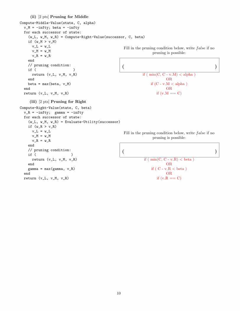
(b) Reasoning in belief space. Now we’ll consider making sequential decisions over time.

We would like to formulate this problem as an MDP. We can model this problem as a partially observed MDP(POMDP), with two states +Bandits and −Bandits indicating the presence and lack of bandits respectively,and two actions Air and Land for sending the shipment by air or by land respectively. Note that the actualstate of this MDP never changes – either there are bandits or there aren’t – so the transition function of thisMDP is just the identity. At each timestep we receive an observation of either +Safe or −Safe, indicatingrespectively that the shipment arrived safely or was lost. The observation and reward models are given inTables 1 and 2b respectively.

One approach to solving POMDPs is to work in terms of the equivalent belief MDP, a new (fully observed)MDP whose state space is the space of distributions over the states of the real-world MDP. In our case, eachdistribution is specified by a real number b giving the probability that there are bandits in the jungle, so thestate space of the belief MDP is the continuous interval [0, 1]. Our uniform prior belief corresponds to a startstate of b0 = 0.5 in the belief MDP.

(i) [2 pts] Suppose we send the first shipment by land. Based on our starting belief state, what is theprobability the shipment arrives safely?

We need to estimate the probability of the shipment arriving safely if there are bandits and if there arenot bandits. We then weight these two outcomes based on our belief.

P (+Safe|+Bandits, Land) = 0.1

P (+Safe| −Bandits, Land) = 0.8

P (+Safe) = P (+Safe|+Bandits, Land)P (+Bandits) + P (+Safe| −Bandits, Land)P (−Bandits)0.5 · 0.1 + 0.5 · 0.8 = 0.45

(ii) [2 pts] After shipping by land we will observe either o1 = +Safe or o1 = -Safe, and based on this observationwill transition to a new belief state b1 = P (s = +Bandits|o1). Give the updated belief state b1 for eachoutcome:

Outcome b1

o1 = +Safe 0.1·0.50.1·0.5+0.8·0.5 = 1/9

o1 =-Safe 0.9·0.50.9·0.5+0.2·0.5 = 9/11

Here we are trying to calculate P (s = +Bandits|o1) based on two different values for the observation o1.This expands to:P (s=+Bandits,o1)

P (o1)

The key thing to remember is that there are two different ways to observe o1, which we expand into:P (s=+Bandits,o1)

P (o1|+Bandits)P (+Bandits) + P (o1|−Bandits)P (−Bandits)

Filling in the expressions for o1 = +Safe and −Safe give you the above expressions.

14

(iii) [4 pts] Give the general transition function P (bt+1|bt, a) for the belief MDP. That is, in the outcome treebelow, label each leaf node in the tree below with an expression for the updated belief bt+1 at that nodein terms of an original belief bt, and also give the probability of reaching that node. Note that an airshipment provides no information and so doesn’t change your beliefs, so we have labeled those branchesfor you as an example.

01

a = Air a = Land

o = +Safe o = -Safe o = +Safe o = -Safe

For +Safe:

bt+1 = 0.1·b0.1·b+0.8·(1−b)

P (bt+1|s, a) = 0.1 · b+ 0.8 · (1− b)

For -Safe:

bt+1 = 0.9·b0.9·b+0.2·(1−b)

P (bt+1|s, a) = 0.9 · b+ 0.2 · (1− b)

15

(a) (b)

Figure 2

(c) [2 pts] Value functions. Suppose that Figure 2a shows, for some discount factor γ, the optimal Q-values forboth actions plotted as a function of the belief b. Which of the plots in Figure 2b gives the value function V (b)?

© Top left © Top right Bottom left © Bottom right

The Value of a state is the max of all Q values; hence, max-ing over the above Q value lines gives the bottomleft graph.

(d) Discounting.

(i) [2 pts] You observe two other agents A and B acting in this belief MDP. All you see are their actionsequences:

Agent A: Land, Land,Air,Air,Air,Air, . . . (followed by Air forever)Agent B: Land,Air,Air,Air,Air,Air, . . . (followed by Air forever)

Supposing that these are rational agents, planning with an infinite time horizon and using the rewardmodel from Table 2b, what if anything can you conclude about their discount factors γA and γB?

γA > γB © γA = γB © γA < γB © Cannot draw anyconclusion.

This question asks how the discount factor affects an agent’s tradeoff between exploration and exploitation.The intended answer was that because large values of γ correspond to greater concern about future rewards,an agent with a larger gamma value is more willing to take exploratory moves that are less immediatelyprofitable. However, because we didn’t specify the observations received by the two agents, we alsoaccepted “Cannot draw any conclusion” as a correct answer, since in the case where Agent A’s first Landshipment arrives safely we’d expect them to try Land again regardless of their discount factor. (sincea safe arrival can only decrease the belief in bandits and thus increase the expected utility of a Landshipment)

16

(a) (b) (c)

(d) (e) (f)

Figure 3: Q-values as a function of belief state.

(ii) [3 pts] The plots in Figure 3 claim to show the optimal Q-values for each action as a function of the beliefstate b (i.e. the probability that bandits are present), under an infinite time horizon with some discountfactor γ. In reality, three of the graphs contain the true Q-values for γ = 0, γ = 0.5, and γ = 0.9, whilethe other three graphs are totally made up and don’t correspond to Q-values under any value of γ. Eachintersection between the two Q-functions is labeled with the belief state at that point. Note that the plotsare intended to show qualitative behavior, so different plots do not necessarily have the same scale on they-axis.

For each value of the discount γ, fill in a single circle indicating which plot contains the Q-values underthat discount. This question can be answered without any computation.

γ = 0: © (a) (b) © (c) © (d) © (e) © (f)

γ = .5: (a) © (b) © (c) © (d) © (e) © (f)

γ = .9: © (a) © (b) © (c) © (d) (e) © (f)

The expected utility of a Land shipment decreases as the probability of bandits increases, which rulesout (c), (d), and (f). To distinguish between (a), (b), and (e), note that if it is ever optimal to ship byAir, then it will continue being optimal forever, since shipping by Air doesn’t change the belief state.Thus there is some belief threshold above which the agent will always ship by Air, and below which theagent will ship by Land until enough shipments are lost to drive its belief in bandits above the threshold.Agents with higher discount factors will have a higher threshold, because larger values of γ correspondto planning further into the future: the more future shipments you anticipate having to make, the moreimportant it is to be certain that bandits are present before you commit to making all of those shipmentsby Air instead of Land. So we can order (b), (a), (e) by increasing thresholds 0.43, 0.56, 0.78 to infertheir respective discount factors.

17

Q8. [12 pts] Bayes’ Nets Representation(a) The figures below show pairs of Bayes’ Nets. In each, the original network is shown on the left. The reversed

network, shown on the right, has all the arrows reversed. Therefore, the reversed network may not be able torepresent all of the distributions that the original network is able to represent.

For each pair, add the minimal number of arrows to the reversed network such that it is guaranteed to beable to represent all the distributions that the original network is able to represent. If no arrows need to beadded, clearly write “none needed.”

The reversal of common effects and common causes requires more arrows so that the dependence of children(with parents unobserved) and the dependence of parents (with a common child observed) can be captured.

To guarantee that a Bayes’ net B′ is able to represent all of the distributions of an original Bayes’ net B, B′

must only make a subset of the independence assumptions in B. If independences are in B′ that are not in B,then the distributions of B′ have constraints that could prevent it from representing a distribution of B.

(i) [2 pts]

A

B

C A

B

COriginal Reversed

(ii) [2 pts]

A

B

C A

B

COriginal Reversed

(iii) [2 pts]

(b) For each of the following Bayes’ Nets, add the minimal number of arrows such that the resulting structure isable to represent all distributions that satisfy the stated independence and non-independence constraints (notethese are constraints on the Bayes net structure, so each non-independence constraint should be interpreted asdisallowing all structures that make the given independence assumption). If no arrows are needed, write “noneneeded.” If no such Bayes’ Net is possible, write “not possible.”

Use a pencil or think twice! Make sure it is very clear what your final answer is.

(i) [2 pts] Constraints:

� A ⊥⊥ B� not A ⊥⊥ B | {C}

(ii) [2 pts] Constraints:

� A ⊥⊥ D | {C}� A ⊥⊥ B� B ⊥⊥ C� not A ⊥⊥ B | {D}

A-C edge can be flipped.

(iii) [2 pts] Constraints:

� A ⊥⊥ B� C ⊥⊥ D | {A,B}� not C ⊥⊥ D | {A}� not C ⊥⊥ D | {B}

18

Q9. [11 pts] Preprocessing Bayes’ Net Graphs for Inference

For (a) and (b), consider the Bayes’ net shown on the right. You are given thestructure but you are not given the conditional probability tables (CPTs). Wewill consider the query P (B| + d), and reason about which steps in the variableelimination process we might be able to execute based on just knowing the graphstructure and not the CPTs.

A B

D

C

(a) [1 pt] Assume the first variable we want to eliminate is A and the resulting factor would be f1(B). Mark whichone of the following is true.

© f1(+b) = f1(−b) = 1

© f1(+b) = f1(−b) = 0

f1(B) cannot be computedfrom knowing only the graphstructure.

© f1(B) can be computedfrom knowing only the graphstructure but is not equal toany of the provided options.

B depends on A and the factor f1(B) depends on the distribution of A.

(b) [1 pt] Assume the first variable we eliminate is C and the resulting factor is g1(B). Mark which one of thefollowing is true.

g1(+b) = g1(−b) = 1

© g1(+b) = g1(−b) = 0

© g1(B) cannot be computedfrom knowing only the graphstructure.

© g1(B) can be computedfrom knowing only the graphstructure but is not equal toany of the provided options.

Eliminating C involves summing over a conditional distribution and a marginal distribution, both of which mustbe equal to 1 since they are distributions. Algebraically, g1(+b) =

∑c P (c|+ b)P (c) =

∑c P (c|+ b)

∑c P (c) =

(1)(1) and g1(−b) is analogous.

For (c) through (g), consider the Bayes’ net shown on the right. You are given thestructure but you are not given the conditional probability tables (CPTs). We willconsider the query P (B|+ g), and again we will reason about which steps in thevariable elimination process we might be able to execute based on just knowingthe graph structure and not the CPTs.

A B

E

C

D F

G

The reasoning for these questions is the same as the previous.

(c) [1 pt] Assume the first variable we eliminate is D and the resulting factor is h1(A). Mark which one of thefollowing is true.

h1(+a) = h1(−a) = 1

© h1(+a) = h1(−a) = 0

© h1(A) cannot be computedfrom knowing only the graphstructure.

© h1(A) can be computedfrom knowing only the graphstructure but is not equal toany of the provided options.

(d) [1 pt] Assume the first 2 variables we eliminate are A and D and the resulting factor is i2(B). Mark which oneof the following is true.

© i2(+b) = i2(−b) = 1

© i2(+b) = i2(−b) = 0

i2(B) cannot be computedfrom knowing only the graphstructure.

© i2(B) can be computedfrom knowing only the graphstructure but is not equal toany of the provided options.

19

(e) [1 pt] Assume the first variable we eliminate is F and the resulting factor is j1(C). Mark which one of thefollowing is true.

j1(+c) = j1(−c) = 1

© j1(+c) = j1(−c) = 0

© j1(C) cannot be computedfrom knowing only the graphstructure.

© j1(C) can be computedfrom knowing only the graphstructure but is not equal toany of the provided options.

20

A B

E

C

D F

G

For your convenience we included the Bayes’ Net structure again on this page.

(f) [1 pt] Assume the first 2 variables we eliminate are Fand C and the resulting factor is k2(B). Mark which oneof the following is true.

k2(+b) = k2(−b) = 1

© k2(+b) = k2(−b) = 0

© k2(B) cannot be computedfrom knowing only the graphstructure.

© k2(B) can be computedfrom knowing only the graphstructure but is not equal toany of the provided options.

(g) [1 pt] Assume the first variable we eliminate is E and the resulting factor is l1(B,+g). Mark which one of thefollowing is true.

© l1(+b,+g) = l1(−b,+g) =1

© l1(+b,+g) = l1(−b,+g) =0

l1(B,+g) cannot be com-puted from knowing only thegraph structure.

© l1(B,+g) can be computed

from knowing only the graphstructure but is not equal toany of the provided options.

21

(h) [4 pts] In the smaller examples in (a) through (g) you will have observed that sometimes a variable can beeliminated without knowing any of the CPTs. This means that variable’s CPT does not affect the answer tothe probabilistic inference query and that variable can be removed from the graph for the purposes of thatprobabilistic inference query. Now consider the following, larger Bayes’ net with the query P (Q|+ e).Variables that are not in the union of the ancestors of the query and ancestors of the evidence can be pruned.Summing them out gives a constant factor of 1 that can be ignored. Verify this yourself for the variablesmarked.

M

P Q

R

H

L

F

K

N

J

O

G I

BA D EC

Mark all of the variables whose CPTs do not affect the value of P (Q|+ e):

© A © B C D © E

F © G H © I J

K L © M N O

P © Q R

22

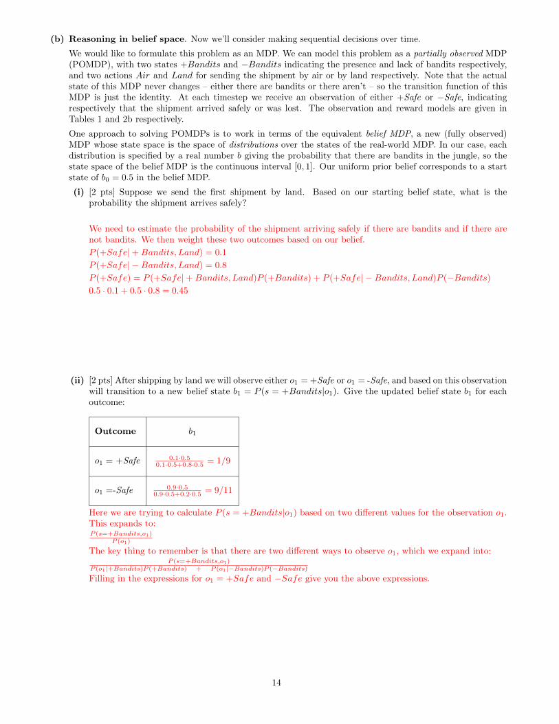
Q10. [8 pts] Clustering

In this question, we will do k-means clustering to clusterthe points A,B . . . F (indicated by ×’s in the figure on theright) into 2 clusters. The current cluster centers are Pand Q (indicated by the � in the diagram on the right).Recall that k-means requires a distance function. Given 2points, A = (A1, A2) and B = (B1, B2), we use the follow-ing distance function d(A,B) that you saw from class,

d (A,B) = (A1 −B1)2 + (A2 −B2)2

−4 −3 −2 −1 0 1 2 3 4−3

−2

−1

0

1

2

3

4

A(0, 0)

B(−1, 2)

C(−2, 1)

D(−1, −2)

E(3, 3)

F(1, 1)

P(−3, 0)

Q(2, 2)

(a) [2 pts] Update assignment step: Select all points that get assigned to the cluster with center at P :

© A B C D © E © F © No point gets assigned to cluster P

(b) [2 pts] Update cluster center step: What does cluster center P get updated to?The cluster center gets updated to the point, P ′ which minimizes, d(P ′, B) +d(P ′, C) +d(P ′, D), which in thiscase turns out to be the centroid of the points, hence the new cluster center is(

−1− 2− 1

3,

2 + 1− 2

3

)=

(−4

3,

+1

3

)

Changing the distance function: While k-means used Euclidean distance in class, we can extend it to otherdistance functions, where the assignment and update phases still iteratively minimize the total (non-Euclidian)distance. Here, consider the Manhattan distance:

d′ (A,B) = |A1 −B1|+ |A2 −B2|

We again start from the original locations for P and Q as shown in the figure, and do the update assignment stepand the update cluster center step using Manhattan distance as the distance function:

(c) [2 pts] Update assignment step: Select all points that get assigned to the cluster with center at P , underthis new distance function d′(A,B).

A © B C D © E © F © No point gets assigned to cluster P

(d) [2 pts] Update cluster center step: What does cluster center P get updated to, under this new distancefunction d′(A,B)?

The cluster center gets updated to the point, P ′ which minimizes, d′(P ′, A) + d′(P ′, C) + d′(P ′, D), which inthis case turns out to be the point with X-coordinate as the median of the X-coordinate of the points in thecluster and the Y-coordinate as the median of the Y-coordinate of the points in the cluster. Hence the newcluster center is

(−1, 0)

23

Q11. [6 pts] Decision TreesYou are given points from 2 classes, shown as +’s and ·’s. For each of the following sets of points,

1. Draw the decision tree of depth at most 2 that can separate the given data completely, by filling in binarypredicates (which only involve thresholding of a single variable) in the boxes for the decision trees below. Ifthe data is already separated when you hit a box, simply write the class, and leave the sub-tree hanging fromthat box empty.

2. Draw the corresponding decision boundaries on the scatter plot, and write the class labels for each of theresulting bins somewhere inside the resulting bins.

If the data can not be separated completely by a depth 2 decision tree, simply cross out the tree template. We solvethe first part as an example.

−0.5 0 0.5 1 1.5 2−2

−1.5

−1

−0.5

0

f1

f 2

← Decision Boundary PlusDot

f < 0.5

Dot Plus

YES NO

YES YESNO NO

1

−1 0 1 2 3

−1

−0.5

0

0.5

1

1.5

2

2.5

3

f1

f 2

f < 1

f < 1 Dot

Plus Dot

YES NO

YES YESNO NO

1

2

−1 0 1 2 3

−2

−1.5

−1

−0.5

0

0.5

1

1.5

2

f1

f 2

YES NO

YES YESNO NONot separable usin

g a depth 2

decision tre

e

−4 −2 0 2 4

−4

−3

−2

−1

0

1

2

3

4

f1

f 2

f < 0

f < -2 f < 2

Plus Dot Dot Plus

YES NO

YES YESNO NO

2

1 1

24

Q12. [10 pts] Machine Learning: OverfittingSuppose we are doing parameter estimation for a Bayes’ net, and have a training set and a test set. We learn themodel parameters (probabilities) from the training set and consider how the model applies to the test set. In thisquestion, we will look at how the average log likelihood of the training dataset and the test dataset varies as afunction of the number of samples in the training dataset.

Consider the Bayes’ net shown on the right. Let x1 . . . xm be them training samples, andx′1 . . . x

′n be the n test samples, where xi = (ai, bi). Recall that once we have estimated

the required model parameters (conditional probability tables) from the training data,the likelihood L for any point xi is given by:

L(xi) = P (xi) = P (ai)P (bi|ai)

We additionally define the log-likelihood of the point xi, to be LL(xi) = log(L(xi)).

A B

We use the log likelihood for a single point to define the average log likelihood on the training set (LL-Train) andthe test set (LL-Test) as follows:

LL-Train =1

m

m∑i=1

LL(xi) =1

m

m∑i=1

log (L(xi)) =1

m

m∑i=1

log (P (ai)P (bi|ai))

LL-Test =1

n

n∑i=1

LL(x′i) =1

n

n∑i=1

log (L(x′i)) =1

n

n∑i=1

log (P (a′i)P (b′i|a′i))

We assume the test set is very large and fixed, and we will study what happens as the training set grows.

Consider the following graphs depicting the average log likelihood on the Y-axis and the number of training exampleson the X-axis.

1 2 3 4 5 6 7 8 9 10111213141516

s

r

Number of training examples

Aver

age

log l

ikel

ihood

Average Train Log Likelihood, LL−Train

Average Test Log Likelihood, LL−Test

(a) A

1 2 3 4 5 6 7 8 9 10111213141516s

r


Aver

age

log l

ikel

ihood



(b) B

1 2 3 4 5 6 7 8 9 10111213141516s

r


Aver

age

log l

ikel

ihood



(c) C

1 2 3 4 5 6 7 8 9 10111213141516s

r


Aver

age

log l

ikel

ihood



(d) D

1 2 3 4 5 6 7 8 9 10111213141516r

s



(e) E

1 2 3 4 5 6 7 8 9 10111213141516

s

r


Aver

age

log l

ikel

ihood



(f) F

(a) [2 pts] Which graph most accurately represents the typical behaviour of the average log likelihood of the trainingand the testing data as a function of the number of training examples?

© A © B C © D © E © F

Note: the solution assumes that the test and training samples are identically distributed. If this is not the case

25

(as can be in reality due to cost, opportunity, etc.), then the train likelihood will converge but the test likelihoodcould improve then decrease if there is overfitting.

With only scarce data, the training data is overfit, and test performance is poor due to little data and overfitting.As more data is gathered the training data is no longer fit perfectly, but the model does approach the exactdistribution of the data from which the test and training were sampled. In this way both log-likelihoodsconverge to the average log-likelihood under the distribution of the data (which turns out to be equivalent tothe negative of the entropy).

(b) [2 pts] Suppose our dataset contains exactly one training example. What is the value of LL-Train?

© −∞

© 1/2

© −2

© 1

© −1

© 2

© −1/2

© ∞

0

© Can be determined but is not equal to any ofthe provided options

© Cannot be determined from the informationprovided

The learned model will put all of its probability mass on that one example, giving it probability 1, thuslog-probability 0.

(c) [3 pts] If we did Laplace Smoothing with k = 5, how would the values of LL-Train and LL-Test change in thelimit of infinite training data? Mark all that are correct.

LL-Train would remain the same.

© LL-Train would go up.

© LL-Train would go down.

LL-Test would remain the same.

© LL-Test would go up.

© LL-Test would go down.

In the limit of inifinite data, Laplace smoothing does not change the parameter estimates. Laplace smoothingis equivalent to adding fake training examples for all possible outcomes, and in this case since we already haveinfinite data, the small number of examples added do not change anything.

(d) [3 pts] Consider the following increasingly complex Bayes’ nets: G1, G2, and G3.

U V W U V W U V W

G1 G2 G3

Consider the following graphs which plot the test likelihood on the Y-axis for each of the Bayes’ nets G1, G2,and G3

Model Complexity Model Complexity

A B C

G1 G2 G3

Model ComplexityG1 G2 G3 G1 G2 G3

.. .

Test

Set

Log

Lik

elih

ood

Test

Set

Log

Lik

elih

ood

Test

Set

Log

Lik

elih

ood

. ..

.. .

26

For each scenario in the column on the left, select the graph that best matches the scenario. Pick each graphexactly once.

Small amount of training data: © A B © C

Medium amount of training data: A © B © C

Large amount of training data: © A © B C

For a small amount of data, a simpler Bayes’ net (one with fewer edges, thus making more independenceassumptions) generalizes better, whereas a complex Bayes’ net would overfit. For a large amount of trainingdata, the simpler Bayes’ net would underfit whereas the more complex Bayes’ net would converge to the truedistribution.

27

Documents

CS 188 Arti cial Intelligence Final - Amazon S3 · Arti cial Intelligence Final You have approximately 3 hours. The exam is closed book, closed notes except your three one-page crib