Crustal VS structure in northwestern Canada: Imaging … · Crustal VS structure in northwestern Canada: Imaging the Cordillera‐craton transition with ambient noise tomography

Crustal VS structure in northwestern Canada: Imagingthe Cordillera‐craton transition with ambient noise tomography

Colleen A. Dalton,1 James B. Gaherty,2 and Anna M. Courtier3

Received 29 April 2011; revised 10 October 2011; accepted 12 October 2011; published 24 December 2011.

[1] Crustal seismic velocity structure in northwest Canada is imaged using group velocitymeasurements derived from ambient noise cross correlations. The focus area surrounds theCanadian Northwest Experiment (CANOE) array, a 16 month deployment of 59broadband seismic stations. The CANOE array extended from the Northern Cordilleraon the west into the Archean Slave province to the east, crossing crustal terranes that span∼4 Gyr of Earth history. Forty broadband stations from the Canadian NationalSeismograph Network and the POLARIS network are also included. The Green’sfunction for each pair of stations is estimated by cross‐correlating 24 h long time series ofambient noise for each day in the time period July 2004 to June 2005. Fundamental modeRayleigh waves are observed on cross‐correlated vertical component records and Lovewaves on the transverse components. The group velocity measurements are inverted for3‐D shear wave velocity within the crust. Local sensitivity kernels are used to accountfor the effects of a laterally variable sedimentary layer at shallow depths, and receiverfunction P‐s differential times at the CANOE stations constrain total crustal thickness.Known sedimentary basins dominate lateral variations in wave speed in the shallow crust.In the middle crust, the model contains a strong low‐velocity region that correlatesspatially with the location of Proterozoic metasedimentary rocks that have been inferredfrom active source reflection profiles to occupy much of the crust beneath the Cordilleranterranes. Velocity variations in the lower crust, which are weakly resolved due to thelimited period range of our data set (5–20 s), suggest a west‐to‐east transition from lowerto higher wave speeds that aligns with the Cordilleran deformation front in parts of thestudy area. The results presented here are consistent with but do not confirm the notionof Proterozoic strata throughout much of the Cordilleran crust. These metasedimentaryrocks, if present, must have experienced some deformation and metamorphism in order toalso be consistent with upper mantle seismic models that contain a sharp transition fromlow to high velocity across the deformation front.

Citation: Dalton, C. A., J. B. Gaherty, and A. M. Courtier (2011), Crustal VS structure in northwestern Canada: Imaging theCordillera‐craton transition with ambient noise tomography, J. Geophys. Res., 116, B12315, doi:10.1029/2011JB008499.

1. Introduction

[2] The tectonic evolution of northwestern Canada spansseveral billion years of Earth history, and it presents an idealenvironment for studying the processes of continentalaccretion and growth. In this paper, we use ambient noisecross correlation to derive a new three‐dimensional model ofcrustal shear wave velocity for the region. We utilize broad-band stations from the Canadian Northwest Experiment(CANOE), the Canadian National Seismograph Network

(CNSN), and the Portable Observatories of LithosphericAnalysis and Research Investigating Seismicity (POLARIS).We compare our results to detailed images of the subsur-face along active source reflection and refraction transectsacross the region, which were gathered as part of theLithoprobe Slave‐Northern Cordillera Lithospheric Evolu-tion (SNORCLE) project [Cook and Erdmer, 2005]. Thesurface waves measured with ambient noise cross corre-lation have a larger wavelength and do not resolve such finedetails, but they allow coverage over a much larger area,thereby complementing the scale of information provided bythe reflection and refraction lines.[3] The ability to image the Earth’s subsurface with the

seismic ambient noise field has provided valuable newconstraints on the crust and upper mantle in many regionsacross the globe [e.g., Shapiro et al., 2005; Harmon et al.,2007; Lin et al., 2008; Yao et al., 2009]. The primaryadvantage of ambient noise tomography is the lack ofdependence on earthquake occurrence; all that is needed are

1Department of Earth Sciences, BostonUniversity, Boston,Massachusetts,USA.

2Lamont‐Doherty Earth Observatory, Earth Institute at ColumbiaUniversity, Palisades, New York, USA.

3Department of Geology and Environmental Science, James MadisonUniversity, Harrisonburg, Virginia, USA.

Copyright 2011 by the American Geophysical Union.0148‐0227/11/2011JB008499

JOURNAL OF GEOPHYSICAL RESEARCH, VOL. 116, B12315, doi:10.1029/2011JB008499, 2011

B12315 1 of 30

http://dx.doi.org/10.1029/2011JB008499

pairs of receivers that were active for the same period oftime, although not every station pair will provide usefuldata. Ambient noise tomography thus requires no a prioriknowledge of earthquake source properties and allows theinclusion of paths that are not sampled by typical earthquakestation geometries. Furthermore, higher‐resolution imagesare possible because of the short receiver‐receiver paths, andbecause ambient noise surface waves are of higher fre-quency (and smaller wavelength) than those used for tradi-tional tomographic studies. The primary disadvantages ofambient noise tomography are that (1) assumptions must bemade about the distribution of noise sources [e.g., Tsai,2009]; (2) continuous time series over a long time periodare required; and (3) ambient noise cross correlation pro-vides useful data in a restricted frequency range. The Earth’sbackground seismic noise level is especially high in themicroseism band: the double‐frequency band (0.14–0.2 Hz)and the single‐frequency band (0.05–0.1 Hz) [e.g., Webb,1998].[4] Ambient noise tomography presents a distinct advan-

tage in northwestern Canada, where earthquakes are few andhave an uneven geographical distribution. The strongmicroseism band allows imaging with surface waves in theperiod range 5–25 s, which allows us to probe the prove-nance of crustal structure across the margin of the NorthAmerican craton and beneath the northern Cordillera. Insection 2, we present a brief overview of the geologic settingin the study area, including the critical questions related tocrustal provenance. In sections 3 and 4, the analysis of

data and measurement of surface wave group velocity aredescribed, and two‐dimensional group speed maps arederived in section 5. The three‐dimensional model of crustalshear wave speeds is the subject of section 6, and section 7contains the tectonic interpretation of the model. Tests ofthe model robustness and resolution are presented inAppendix A.

2. Tectonic Setting

[5] From east to west, the study region (Figure 1) can bedivided into three sections by age: Archean, Proterozoic,and Phanerozoic [Hoffman, 1988]. The Archean Slavecraton, a nucleus of the Canadian Shield, was assembled overthe time period 4.0–2.6 Ga. It consists of the Contwoytoterrane to the east and the Anton terrane in the west, whichhosts some of the oldest rocks on Earth, the Acasta gneiss[Bowring and Williams, 1999]. The Proterozoic Wopmayorogen formed between 2.1–1.84 Ga; it is comprised of threedistinct elements [Hildebrand et al., 1987]. The Hottah ter-rane was a magmatic arc that formed west of the Slave cratonfrom 1.92–1.90 Ga. It and its associated sedimentary rocksconverged with the western Slave province during 1.90–1.88 Ga, in the process shortening and displacing theCoronation sedimentary rocks that had formed west of theextensional continental margin. The Great Bear magmaticarc formed on top of the Hottah and Coronation terranesbetween 1.88 and 1.84 Ga as a consequence of eastwardsubduction beneath the continental margin. The westernmost

Figure 1. (left) Topography of the study area. Seismic stations shown with white symbols (circles,CANOE (legs A, B, and C); triangles, CNSN; squares, POLARIS). White box outlines the area imagedin this study. Solid black lines indicate the Tintina fault and Great Slave Lake shear zone; barbed lineindicates the Cordilleran Deformation Front. The Bowser (BB) and Nechako (NB) sediment basins areoutlined in blue. The dashed yellow line indicates the eastern extent of the Western Canada SedimentaryBasin; the solid yellow and orange lines indicate sediment thickness of 3000 and 4000 m, respectively.(right) Geology of the study area. Green: Archean Slave craton; from bright to dark green (west to east)are the Coronation, Anton, and Contwoyto domains. Red shows Proterozoic Wopmay orogen; from brightto dark red are the Nahanni, Fort Simpson, Hottah, and Great Bear domains. Bright to dark magentashows the Proterozoic Ksituan and Chincaga, Buffalo Head, and Taltson terranes, and the ArcheanRae province. Bright to pale yellow shows the Phanerozoic Foreland, Omineca, Intermontane, Coast,and Insular Belts. Blue lines indicate the four SNORCLE reflection/refraction lines.

DALTON ET AL.: CRUSTAL VELOCITY IN NW CANADA B12315B12315

2 of 30

element of the Wopmay orogen, the Fort Simpson terrane,was formed as a magmatic arc at ∼1.85 Ga and collided withthe western margin of the Hottah terrane sometime prior to1.71 Ga. As much of the Wopmay orogen is today coveredby Phanerozoic sedimentary rocks of the Western CanadaSedimentary Basin, the boundaries between Proterozoicdomains have been inferred from drilling and potentialfield data.[6] Following the accretion of these terranes, the region

experienced episodes of extension, during which deepbasins of sediments formed, and periods of deformation thatcompressed and uplifted rocks locally during 1.7–0.6 Ga.Beginning in the Jurassic, the Canadian Cordillera was builtthrough accretion of terranes onto the North Americancraton. This process produced westward growth of the NorthAmerican continent, and the resulting structures are todaysubdivided into five parallel northwestwardly trending belts[e.g., Creaser and Spence, 2005]. To the east, the Forelandfold‐and‐thrust belt is interpreted to be thick sedimentarysequences that were detached from the cratonic basementand thrust eastward onto the continental margin duringcollision between North America and oceanic terranes. Themetamorphic and granitic Omineca belt separates theForeland belt from the Intermontane belt to its west andlikely formed as oceanic rocks and continental and mag-matic arcs were caught in the middle of Jurassic collisionbetween the Intermontane superterrane and North America.It is interpreted to represent the boundary between ancens-tral North America and the newer, accreted terranes. TheIntermontane belt is composed of sedimentary and volcanicrocks that show little affinity with the crustal rocks ofancestral North America. During the middle Cretaceous, theexotic Insular terrane accreted to the continent, deformingthe orogen and producing the Coast belt, a plutonic suturezone that today contains the Coast and Cascade mountains.[7] This margin‐parallel accretional pattern is sliced by

two major translational features (Figure 1): the strike‐slipTintina fault and Great Slave Lake shear zone. Estimates ofthe total displacement along the right‐lateral Cenozoic eraTintina fault are summarized by Zelt et al. [2006] and rangefrom 425 km to 2000 km. The Great Slave Lake shear zoneis zone of mylonites 25 km wide that accommodated right‐lateral slip during the Proterozoic [Hoffman, 1987]. Portionsof the tectonic history are obscured by young sedimentarybasins. The Western Canada Sedimentary Basin has athickness of 0 km at its eastern end (the exposed Canadianshield) and thickens to the southwest, obtaining sedimentthicknesses of 6 km in the northwest and 3 km on thewestern edge where it meets the Omineca and Intermontanebelts (Atlas of the WCSB). Within the Cordillera, theBowser basin (and the Sustut basin adjacent to it) was a siteof considerable marine and nonmarine sediment depositionduring ∼170–100 Myr. Today it spans 200 km in width(east‐west) and 400 km in length (north‐south) [Rickettset al., 1992]. Sedimentary strata are likely present todepths of at least 5 km, and tomographic modeling of first‐arrival P waves from SNORCLE reflection lines shows slowP wave speeds (<4 km/s) from the surface to ∼1 km depth[Snyder and Roberts, 2007]. The Nechako Basin, alsoan interior basin located in British Columbia, covers75,000 km2. Because it is overlain by volcanic flows, less isknown about the sedimentary structure, but sediment

thickness is estimated to be ∼3 km in some places [e.g.,Hayward and Calvert, 2009; Calvert and Hayward, 2009].[8] Overall, this large‐scale geologic history of the

Cordillera implies that the North American continent hasgrown substantially during the Phanerozoic. At the litho-spheric scale, this is supported by regional and global uppermantle seismic velocity models that clearly suggest relativelyhigh‐temperature (thermally “young”) lithosphere beneaththe Cordillera that transitions abruptly to cold lithospherebeneath the Proterozoic craton [e.g., Frederiksen et al., 2001;Nettles and Dziewonski, 2008; Mercier et al., 2009].Smaller‐scale geological and geophysical observations havebeen interpreted differently. Proterozoic age rocks outcropin a number of locales throughout the Cordillera, and thepresence of these has been combined with the LithoprobeSNORCLE reflection profiles to suggest that the lower crustand lithosphere of ancestral North America underlie most ofthe northern Canadian Cordillera [Snyder et al., 2002; Cooket al., 2004]. In this scenario, the terranes of the Cordillerawere accreted as a series of thin flakes on top of Proterozoiclithosphere, and with the exception of the upper crust, muchof the Cordilleran crust consists of layered sedimentaryrocks formed during 1.85–0.54 Gyr and underlain byProterozoic basement and lithosphere [e.g., Snyder et al.,2009]. Resolving this discrepancy is necessary for improv-ing models of the growth of the North American continent.Images of crustal shear velocity structure over a broad swathof the craton‐Cordillera transition directly address this issue.

3. Data Processing

[9] We have collected and analyzed data from 59 stationsof the CANOE array, 16 stations of the Canadian NationalSeismograph Network, and 24 stations of the POLARISnetwork. The CANOE array consisted of three “legs” thatextended radially outward from Fort Nelson to the northeast(leg A), the northwest (leg B), and the southeast (leg C)(Figure 1). We collected continuous daily records from allthree components of the seismometers for the time periodJuly 1, 2004 to June 30, 2005, coinciding with the optimaltime window for the CANOE deployment. The data pro-cessing procedure, which follows the steps outlined byBensen et al. [2007], begins with desampling the records to1 sample per second, followed by removal of the daily meanand trend and the instrument response from each compo-nent. The seismograms are band‐pass filtered in the periodrange 5–50 s, and temporal normalization is applied tominimize the signals of earthquakes. We use one‐bit nor-malization and divide each record by its absolute value,which reduces all positive amplitudes to a value of 1 and allnegative amplitudes to a value of −1. As a final step, thedata are spectrally whitened.[10] The daily cross correlations are then computed

between all station pairs. Vertical component records arecross correlated with other vertical records, and transversecomponent records are cross correlated other transverserecords. The transverse component is found by rotating thetwo horizontal components so that one is along the greatcircle path connecting the two stations and the other isperpendicular to the great circle path. The daily cross corre-lations are stacked into a 1month time series, and the monthlycross correlations are further stacked to yield a 1 year record


3 of 30

on which we make group velocity measurements. In con-structing the yearly stack, the monthly stacks are weighted bythe number of days from which the monthly stack was built.This is done so that months for which relatively few dayswere available are given less weight.[11] The vertical component and transverse component

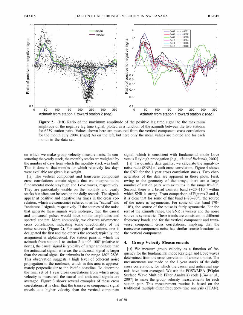
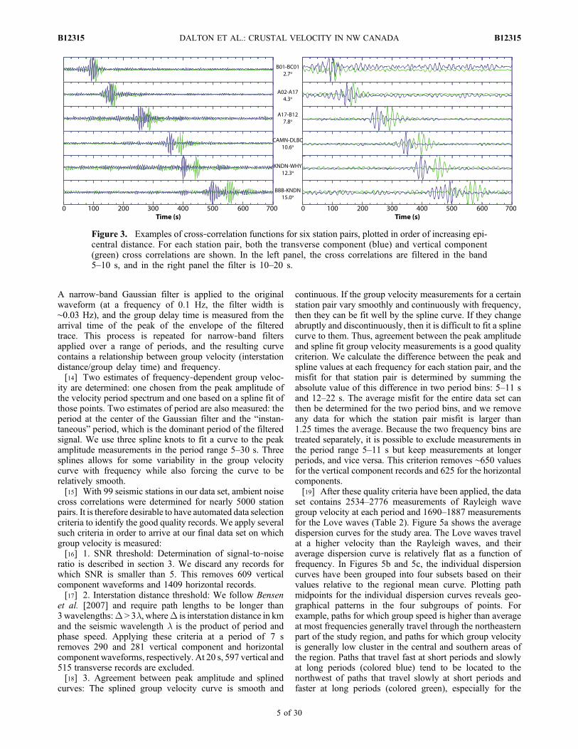
cross correlations contain signals that we interpret to befundamental mode Rayleigh and Love waves, respectively.They are particularly visible on the monthly and yearlystacks but often can be seen on the daily records. The signalsappear at positive and negative lag times in the cross cor-relation, which are sometimes referred to as the “causal” and“anticausal” signals, respectively. If the sources of the noisethat generate these signals were isotropic, then the causaland anticausal pulses would have similar amplitudes andspectral content. More commonly, we observe asymmetriccross correlations, indicating some directionality of thenoise sources (Figure 2). For each pair of stations, one isdesignated the first and the other is the second; typically, theassignment is alphabetical. For station pairs in which theazimuth from station 1 to station 2 is ∼0°–100° (relative tonorth), the causal signal is typically of larger amplitude thanthe anticausal signal, whereas the anticausal signal is largerthan the causal signal for azimuths in the range 180°–280°.This observation suggests a high level of coherent noisepropagation to the northeast, which in this area is approxi-mately perpendicular to the Pacific coastline. To determinethe final set of 1 year cross correlations from which groupvelocity is measured, the causal and anticausal signals areaveraged. Figure 3 shows several examples of these crosscorrelations; it is clear that the transverse component signaltravels at a higher velocity than the vertical component

signal, which is consistent with fundamental mode Loveversus Rayleigh propagation [e.g., Aki and Richards, 2002].[12] To quantify data quality, we calculate the signal‐to‐

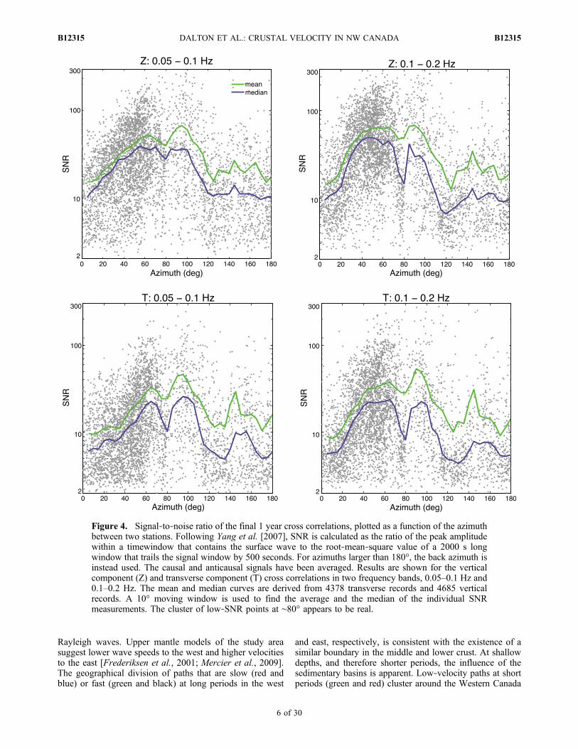
noise ratio (SNR) of each cross correlation. Figure 4 showsthe SNR for the 1 year cross correlation stacks. Two char-acteristics of the data are apparent in these plots. First,owing to the geometry of the arrays, there are a largenumber of station pairs with azimuths in the range 0°–80°.Second, there is a broad azimuth band (∼20–110°) withinwhich SNR is strong. From comparison of Figures 2 and 4,it is clear that for some of that band (∼20–70°), the sourceof the noise is asymmetric. For some of that band (70–110°), the source of the noise is fairly symmetric. For therest of the azimuth range, the SNR is weaker and the noisesource is symmetric. These trends are consistent in differentfrequency bands and for the vertical component and trans-verse component cross correlations, implying that thetransverse component noise has similar source locations asthe vertical component.

4. Group Velocity Measurements

[13] We measure group velocity as a function of fre-quency for the fundamental mode Rayleigh and Love wavesdetermined from the cross correlation of ambient noise. Themeasurements are made on the 1 year stacks of the dailycross correlations, for which the causal and anticausal sig-nals have been averaged. We use the PGSWMFA (PGplotSurface Wave Multiple Filter Analysis) code [Cho et al.,2007] to make the group velocity measurements for eachstation pair. This measurement routine is based on thetraditional multiple‐filter frequency‐time analysis (FTAN).

Figure 2. (left) Ratio of the maximum amplitude of the positive lag time signal to the maximumamplitude of the negative lag time signal, plotted as a function of the azimuth between the two stationsfor 6239 station pairs. Values shown here are measured from the vertical component cross correlationsfor the month July 2004. (right) As on the left, but here only the mean values are plotted and for eachmonth in the data set.


4 of 30

A narrow‐band Gaussian filter is applied to the originalwaveform (at a frequency of 0.1 Hz, the filter width is∼0.03 Hz), and the group delay time is measured from thearrival time of the peak of the envelope of the filteredtrace. This process is repeated for narrow‐band filtersapplied over a range of periods, and the resulting curvecontains a relationship between group velocity (interstationdistance/group delay time) and frequency.[14] Two estimates of frequency‐dependent group veloc-

ity are determined: one chosen from the peak amplitude ofthe velocity period spectrum and one based on a spline fit ofthose points. Two estimates of period are also measured: theperiod at the center of the Gaussian filter and the “instan-taneous” period, which is the dominant period of the filteredsignal. We use three spline knots to fit a curve to the peakamplitude measurements in the period range 5–30 s. Threesplines allows for some variability in the group velocitycurve with frequency while also forcing the curve to berelatively smooth.[15] With 99 seismic stations in our data set, ambient noise

cross correlations were determined for nearly 5000 stationpairs. It is therefore desirable to have automated data selectioncriteria to identify the good quality records. We apply severalsuch criteria in order to arrive at our final data set on whichgroup velocity is measured:[16] 1. SNR threshold: Determination of signal‐to‐noise

ratio is described in section 3. We discard any records forwhich SNR is smaller than 5. This removes 609 verticalcomponent waveforms and 1409 horizontal records.[17] 2. Interstation distance threshold: We follow Bensen

et al. [2007] and require path lengths to be longer than3wavelengths:D > 3l, whereD is interstation distance in kmand the seismic wavelength l is the product of period andphase speed. Applying these criteria at a period of 7 sremoves 290 and 281 vertical component and horizontalcomponent waveforms, respectively. At 20 s, 597 vertical and515 transverse records are excluded.[18] 3. Agreement between peak amplitude and splined

curves: The splined group velocity curve is smooth and

continuous. If the group velocity measurements for a certainstation pair vary smoothly and continuously with frequency,then they can be fit well by the spline curve. If they changeabruptly and discontinuously, then it is difficult to fit a splinecurve to them. Thus, agreement between the peak amplitudeand spline fit group velocity measurements is a good qualitycriterion. We calculate the difference between the peak andspline values at each frequency for each station pair, and themisfit for that station pair is determined by summing theabsolute value of this difference in two period bins: 5–11 sand 12–22 s. The average misfit for the entire data set canthen be determined for the two period bins, and we removeany data for which the station pair misfit is larger than1.25 times the average. Because the two frequency bins aretreated separately, it is possible to exclude measurements inthe period range 5–11 s but keep measurements at longerperiods, and vice versa. This criterion removes ∼650 valuesfor the vertical component records and 625 for the horizontalcomponents.[19] After these quality criteria have been applied, the data

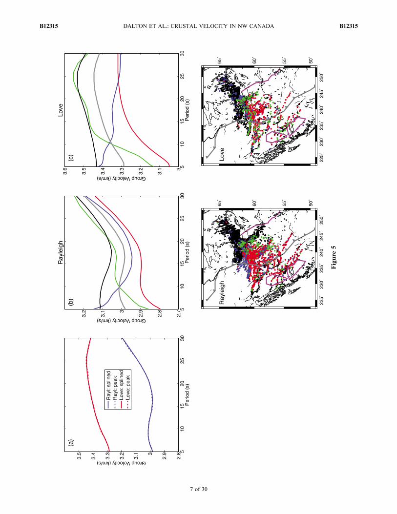
set contains 2534–2776 measurements of Rayleigh wavegroup velocity at each period and 1690–1887 measurementsfor the Love waves (Table 2). Figure 5a shows the averagedispersion curves for the study area. The Love waves travelat a higher velocity than the Rayleigh waves, and theiraverage dispersion curve is relatively flat as a function offrequency. In Figures 5b and 5c, the individual dispersioncurves have been grouped into four subsets based on theirvalues relative to the regional mean curve. Plotting pathmidpoints for the individual dispersion curves reveals geo-graphical patterns in the four subgroups of points. Forexample, paths for which group speed is higher than averageat most frequencies generally travel through the northeasternpart of the study region, and paths for which group velocityis generally low cluster in the central and southern areas ofthe region. Paths that travel fast at short periods and slowlyat long periods (colored blue) tend to be located to thenorthwest of paths that travel slowly at short periods andfaster at long periods (colored green), especially for the

Figure 3. Examples of cross‐correlation functions for six station pairs, plotted in order of increasing epi-central distance. For each station pair, both the transverse component (blue) and vertical component(green) cross correlations are shown. In the left panel, the cross correlations are filtered in the band5–10 s, and in the right panel the filter is 10–20 s.


5 of 30

Rayleigh waves. Upper mantle models of the study areasuggest lower wave speeds to the west and higher velocitiesto the east [Frederiksen et al., 2001; Mercier et al., 2009].The geographical division of paths that are slow (red andblue) or fast (green and black) at long periods in the west

and east, respectively, is consistent with the existence of asimilar boundary in the middle and lower crust. At shallowdepths, and therefore shorter periods, the influence of thesedimentary basins is apparent. Low‐velocity paths at shortperiods (green and red) cluster around the Western Canada

Figure 4. Signal‐to‐noise ratio of the final 1 year cross correlations, plotted as a function of the azimuthbetween two stations. Following Yang et al. [2007], SNR is calculated as the ratio of the peak amplitudewithin a timewindow that contains the surface wave to the root‐mean‐square value of a 2000 s longwindow that trails the signal window by 500 seconds. For azimuths larger than 180°, the back azimuth isinstead used. The causal and anticausal signals have been averaged. Results are shown for the verticalcomponent (Z) and transverse component (T) cross correlations in two frequency bands, 0.05–0.1 Hz and0.1–0.2 Hz. The mean and median curves are derived from 4378 transverse records and 4685 verticalrecords. A 10° moving window is used to find the average and the median of the individual SNRmeasurements. The cluster of low‐SNR points at ∼80° appears to be real.


6 of 30

Figure

5


7 of 30

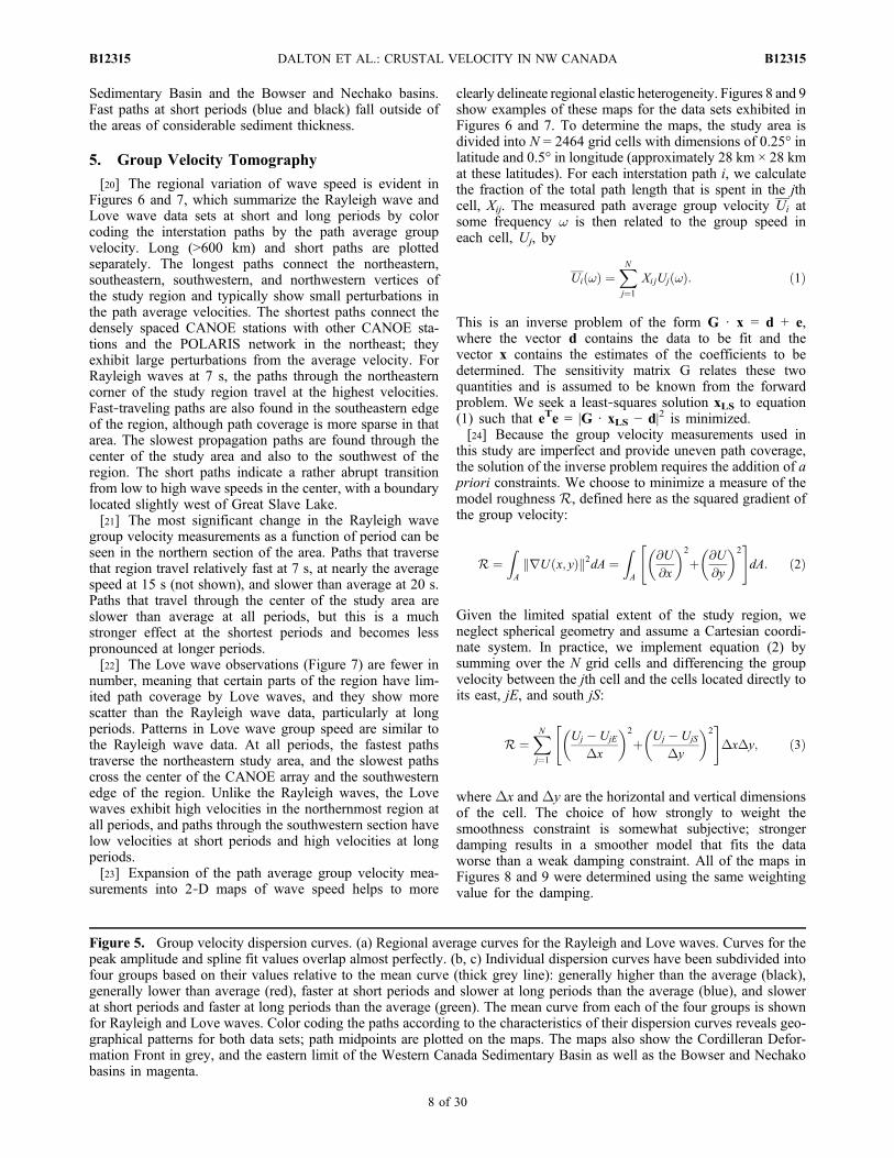
Sedimentary Basin and the Bowser and Nechako basins.Fast paths at short periods (blue and black) fall outside ofthe areas of considerable sediment thickness.

5. Group Velocity Tomography

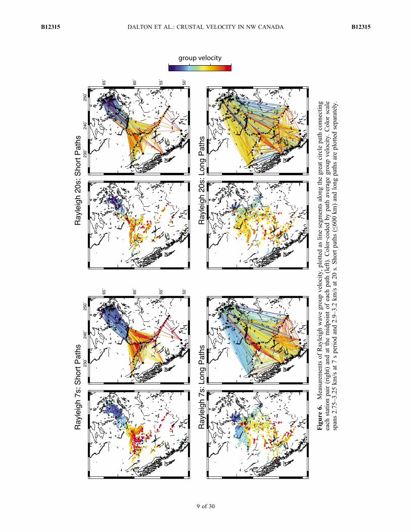
[20] The regional variation of wave speed is evident inFigures 6 and 7, which summarize the Rayleigh wave andLove wave data sets at short and long periods by colorcoding the interstation paths by the path average groupvelocity. Long (>600 km) and short paths are plottedseparately. The longest paths connect the northeastern,southeastern, southwestern, and northwestern vertices ofthe study region and typically show small perturbations inthe path average velocities. The shortest paths connect thedensely spaced CANOE stations with other CANOE sta-tions and the POLARIS network in the northeast; theyexhibit large perturbations from the average velocity. ForRayleigh waves at 7 s, the paths through the northeasterncorner of the study region travel at the highest velocities.Fast‐traveling paths are also found in the southeastern edgeof the region, although path coverage is more sparse in thatarea. The slowest propagation paths are found through thecenter of the study area and also to the southwest of theregion. The short paths indicate a rather abrupt transitionfrom low to high wave speeds in the center, with a boundarylocated slightly west of Great Slave Lake.[21] The most significant change in the Rayleigh wave

group velocity measurements as a function of period can beseen in the northern section of the area. Paths that traversethat region travel relatively fast at 7 s, at nearly the averagespeed at 15 s (not shown), and slower than average at 20 s.Paths that travel through the center of the study area areslower than average at all periods, but this is a muchstronger effect at the shortest periods and becomes lesspronounced at longer periods.[22] The Love wave observations (Figure 7) are fewer in

number, meaning that certain parts of the region have lim-ited path coverage by Love waves, and they show morescatter than the Rayleigh wave data, particularly at longperiods. Patterns in Love wave group speed are similar tothe Rayleigh wave data. At all periods, the fastest pathstraverse the northeastern study area, and the slowest pathscross the center of the CANOE array and the southwesternedge of the region. Unlike the Rayleigh waves, the Lovewaves exhibit high velocities in the northernmost region atall periods, and paths through the southwestern section havelow velocities at short periods and high velocities at longperiods.[23] Expansion of the path average group velocity mea-

surements into 2‐D maps of wave speed helps to more

clearly delineate regional elastic heterogeneity. Figures 8 and 9show examples of these maps for the data sets exhibited inFigures 6 and 7. To determine the maps, the study area isdivided into N = 2464 grid cells with dimensions of 0.25° inlatitude and 0.5° in longitude (approximately 28 km × 28 kmat these latitudes). For each interstation path i, we calculatethe fraction of the total path length that is spent in the jthcell, Xij. The measured path average group velocity Ui atsome frequency w is then related to the group speed ineach cell, Uj, by

Ui !ð Þ ¼XNj¼1

Xi jUj !ð Þ: ð1Þ

This is an inverse problem of the form G · x = d + e,where the vector d contains the data to be fit and thevector x contains the estimates of the coefficients to bedetermined. The sensitivity matrix G relates these twoquantities and is assumed to be known from the forwardproblem. We seek a least‐squares solution xLS to equation(1) such that eTe = |G · xLS − d|2 is minimized.[24] Because the group velocity measurements used in

this study are imperfect and provide uneven path coverage,the solution of the inverse problem requires the addition of apriori constraints. We choose to minimize a measure of themodel roughness R, defined here as the squared gradient ofthe group velocity:

R ¼ZA

rU x; yð Þk k2dA ¼ZA

@U

@x

� �2

þ @U

@y

� �2" #

dA: ð2Þ

Given the limited spatial extent of the study region, weneglect spherical geometry and assume a Cartesian coordi-nate system. In practice, we implement equation (2) bysumming over the N grid cells and differencing the groupvelocity between the jth cell and the cells located directly toits east, jE, and south jS:

R ¼XNj¼1

Uj � UjE

Dx

� �2

þ Uj � UjS

Dy

� �2" #

DxDy; ð3Þ

where Dx and Dy are the horizontal and vertical dimensionsof the cell. The choice of how strongly to weight thesmoothness constraint is somewhat subjective; strongerdamping results in a smoother model that fits the dataworse than a weak damping constraint. All of the maps inFigures 8 and 9 were determined using the same weightingvalue for the damping.

Figure 5. Group velocity dispersion curves. (a) Regional average curves for the Rayleigh and Love waves. Curves for thepeak amplitude and spline fit values overlap almost perfectly. (b, c) Individual dispersion curves have been subdivided intofour groups based on their values relative to the mean curve (thick grey line): generally higher than the average (black),generally lower than average (red), faster at short periods and slower at long periods than the average (blue), and slowerat short periods and faster at long periods than the average (green). The mean curve from each of the four groups is shownfor Rayleigh and Love waves. Color coding the paths according to the characteristics of their dispersion curves reveals geo-graphical patterns for both data sets; path midpoints are plotted on the maps. The maps also show the Cordilleran Defor-mation Front in grey, and the eastern limit of the Western Canada Sedimentary Basin as well as the Bowser and Nechakobasins in magenta.


8 of 30

Figure

6.Measurementsof

Rayleighwavegroupvelocity,p

lottedas

linesegm

entsalongthegreatcirclepath

connectin

geach

stationpair(right)andat

themidpointof

each

path

(left).Color‐coded

bypath

averagegroupvelocity.Color

scale

spans2.75

–3.25km

/sat

7speriod

and2.9–3.2km

/sat

20s.Shortpaths(≤600km

)andlong

pathsareplottedseparately.


9 of 30

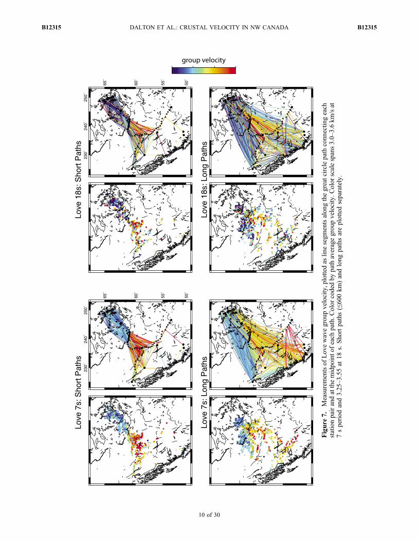
Figure

7.Measurementsof

Lovewavegroupvelocity,plottedas

linesegm

entsalongthegreatcirclepath

connectin

geach

stationpairandatthemidpointo

feach

path.C

olor

codedby

path

averagegroupvelocity.C

olor

scalespans3.0–3.6km

/sat

7speriod

and3.25

–3.55at

18s.Shortpaths(≤600km

)andlong

pathsareplottedseparately.


10 of 30

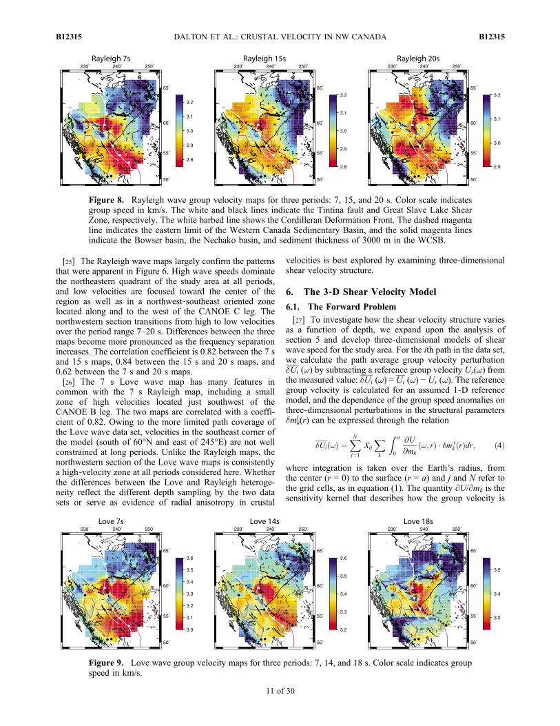
[25] The Rayleigh wave maps largely confirm the patternsthat were apparent in Figure 6. High wave speeds dominatethe northeastern quadrant of the study area at all periods,and low velocities are focused toward the center of theregion as well as in a northwest‐southeast oriented zonelocated along and to the west of the CANOE C leg. Thenorthwestern section transitions from high to low velocitiesover the period range 7–20 s. Differences between the threemaps become more pronounced as the frequency separationincreases. The correlation coefficient is 0.82 between the 7 sand 15 s maps, 0.84 between the 15 s and 20 s maps, and0.62 between the 7 s and 20 s maps.[26] The 7 s Love wave map has many features in

common with the 7 s Rayleigh map, including a smallzone of high velocities located just southwest of theCANOE B leg. The two maps are correlated with a coeffi-cient of 0.82. Owing to the more limited path coverage ofthe Love wave data set, velocities in the southeast corner ofthe model (south of 60°N and east of 245°E) are not wellconstrained at long periods. Unlike the Rayleigh maps, thenorthwestern section of the Love wave maps is consistentlya high‐velocity zone at all periods considered here. Whetherthe differences between the Love and Rayleigh heteroge-neity reflect the different depth sampling by the two datasets or serve as evidence of radial anisotropy in crustal

velocities is best explored by examining three‐dimensionalshear velocity structure.

6. The 3‐D Shear Velocity Model

6.1. The Forward Problem

[27] To investigate how the shear velocity structure variesas a function of depth, we expand upon the analysis ofsection 5 and develop three‐dimensional models of shearwave speed for the study area. For the ith path in the data set,we calculate the path average group velocity perturbation�Ui (w) by subtracting a reference group velocity Ur(w) fromthe measured value: �Ui (w) = Ui (w) − Ur (w). The referencegroup velocity is calculated for an assumed 1‐D referencemodel, and the dependence of the group speed anomalies onthree‐dimensional perturbations in the structural parametersdmk

j (r) can be expressed through the relation

�Ui !ð Þ ¼XNj¼1

Xij

Xk

Z a

0

@U

@mk!; rð Þ � �m j

k rð Þdr; ð4Þ

where integration is taken over the Earth’s radius, fromthe center (r = 0) to the surface (r = a) and j and N refer tothe grid cells, as in equation (1). The quantity ∂U/∂mk is thesensitivity kernel that describes how the group velocity is

Figure 8. Rayleigh wave group velocity maps for three periods: 7, 15, and 20 s. Color scale indicatesgroup speed in km/s. The white and black lines indicate the Tintina fault and Great Slave Lake ShearZone, respectively. The white barbed line shows the Cordilleran Deformation Front. The dashed magentaline indicates the eastern limit of the Western Canada Sedimentary Basin, and the solid magenta linesindicate the Bowser basin, the Nechako basin, and sediment thickness of 3000 m in the WCSB.

Figure 9. Love wave group velocity maps for three periods: 7, 14, and 18 s. Color scale indicates groupspeed in km/s.


11 of 30

influenced by a change in the kth structural parameter. Foran isotropic elastic solid, the shear wave (VS) and com-pressional wave (VP) speed are the structural parametersrequired to describe the elastic properties of any parcel ofmaterial. Because our data set includes both Rayleigh andLove waves, we can also explore whether radial anisotropyis required to satisfy the data. In that case, five independentelastic parameters must be specified: the velocities of hori-zontally and vertically polarized S and P waves VSH, VPH,VSV, VPV, and a fifth parameter h that describes behavior forpolarization angles intermediate between the horizontal andvertical [Dziewonski and Anderson, 1981]. Other variablechoices are possible, but our data are strongly sensitive toVSH and VSV, which guides our choice. The Rayleigh andLove group velocities are also dependent on the density rand the bulk and shear attenuation factors Qk

−1 and Qm−1. It is

impractical to attempt to determine three‐dimensional var-iations in eight parameters, and so we must make somesimplifications. The Love and Rayleigh group velocitieshave little sensitivity to variations in h, r, Qm

−1, and Qk−1; we

choose to ignore variations in these four factors. The dataare considerably more sensitive to variations in VSH and VSV

than in VPH and VPV. We therefore constrain the variationsin VPH and VPV to be proportional to the variations in VSH

and VSV, respectively: dVPH = kdVSH and dVPV = kdVSV,where k = 0.99 [Kustowski et al., 2008].[28] Based on these considerations, equation (4) for the

radially anisotropic case becomes


Xij

Z a

0

@U

@VSH�V j

SH rð Þdr þZ a

0

@U

@VPHk�V j

SH rð Þdr� �

þXNj¼1

Xij

Z a

0

@U

@VSV�V j

SV rð Þdr þZ a

0

@U

@VPVk�V j

SV rð Þdr�

þXLl¼1

@U

@dl�d j

l

�; ð5Þ

where the sensitivity kernels ∂U/∂m depend on frequency wand radius r, and can also vary with horizontal position j. Inequation (5), we have included dependence of the group speedon the depth of radial discontinuities such as the Moho; Lindicates the number of discontinuities and ddl is the pertur-bation in the depth of the lth discontinuity. We followKustowski et al. [2008] and parameterize the model in terms ofisotropic variations dVS and anisotropic variations da, where

�VS ¼ �VSH þ �VSV

2ð6Þ

�a ¼ �VSH � �VSV : ð7Þ

Choosing this parameterization allows us to damp the isotropicand anisotropic variations separately. Equation (5) becomes

�Ui !ð Þ¼XNj¼1

Xij

Z a

0�V j

S rð Þ @U

@VSHþ @U

@VSV

� �þ k

@U

@VPHþ @U

@VPV

� �� dr

þXN

j¼1Xij

Z a

0�aj rð Þ 1

2

@U

@VSH� @U

@VSV

� ��

þ k

2

@U

@VPH� @U

@VPV

� ��dr þ

XL

l¼1

@U

@dl�d j

l

�: ð8Þ

In the following sections, we discuss the choice of referencemodel, the calculation of sensitivity kernels, and parameteri-zation schemes.

6.2. Calculation of Sensitivity Kernels

[29] To calculate the group velocity sensitivity kernels∂U/∂m, we follow the approach of Rodi et al. [1975] anddifferentiate phase velocity sensitivity kernels Km

c = ∂c/∂mwith respect to frequency:

@U

@m¼ U

c2� U

c

� �@c

@mþ !

U2

c2@

@!

@c

@m

� �: ð9Þ

Since phase speed sensitivity kernels can be readily calcu-lated from the eigenfunctions of a specified Earth model[e.g., Takeuchi and Saito, 1972], equation (9) presents aconvenient and numerically efficient expression for deter-mining the group speed kernels. These kernels are approx-imate, requiring numerical differentiation of kernel values @c

@mfor adjacent modes at discrete frequencies. Rodi et al. [1975]showed that the resulting inaccuracies are very small, andwe have verified numerically that these kernels are suffi-ciently accurate and will not introduce bias into our retrievedmodels.[30] The sensitivity kernels are dependent on the choice of

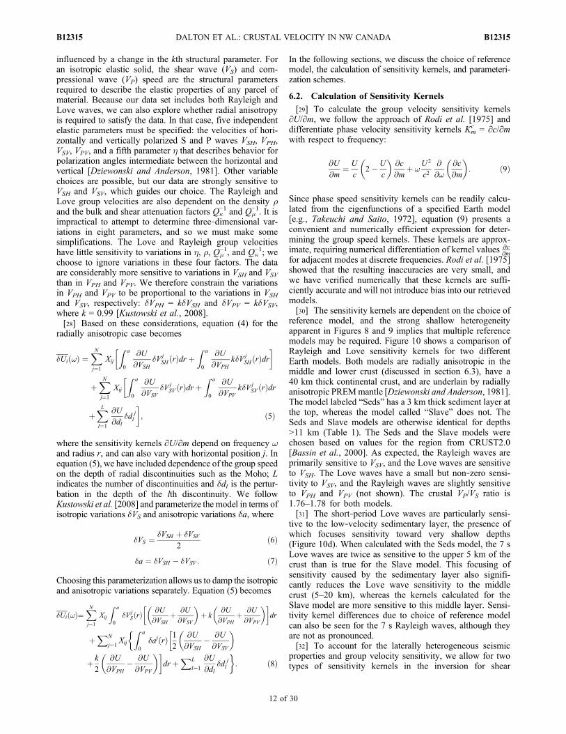
reference model, and the strong shallow heterogeneityapparent in Figures 8 and 9 implies that multiple referencemodels may be required. Figure 10 shows a comparison ofRayleigh and Love sensitivity kernels for two differentEarth models. Both models are radially anisotropic in themiddle and lower crust (discussed in section 6.3), have a40 km thick continental crust, and are underlain by radiallyanisotropic PREMmantle [Dziewonski and Anderson, 1981].The model labeled “Seds” has a 3 km thick sediment layer atthe top, whereas the model called “Slave” does not. TheSeds and Slave models are otherwise identical for depths>11 km (Table 1). The Seds and the Slave models werechosen based on values for the region from CRUST2.0[Bassin et al., 2000]. As expected, the Rayleigh waves areprimarily sensitive to VSV, and the Love waves are sensitiveto VSH. The Love waves have a small but non‐zero sensi-tivity to VSV, and the Rayleigh waves are slightly sensitiveto VPH and VPV (not shown). The crustal VP/VS ratio is1.76–1.78 for both models.[31] The short‐period Love waves are particularly sensi-

tive to the low‐velocity sedimentary layer, the presence ofwhich focuses sensitivity toward very shallow depths(Figure 10d). When calculated with the Seds model, the 7 sLove waves are twice as sensitive to the upper 5 km of thecrust than is true for the Slave model. This focusing ofsensitivity caused by the sedimentary layer also signifi-cantly reduces the Love wave sensitivity to the middlecrust (5–20 km), whereas the kernels calculated for theSlave model are more sensitive to this middle layer. Sensi-tivity kernel differences due to choice of reference modelcan also be seen for the 7 s Rayleigh waves, although theyare not as pronounced.[32] To account for the laterally heterogeneous seismic

properties and group velocity sensitivity, we allow for twotypes of sensitivity kernels in the inversion for shear


12 of 30

velocity structure. Figure 10b shows the gridded region ofour study area and the classification of each cell by type.The choice of reference model for each grid cell is guided bythe sediment thickness values from SEDMAP [Laske and

Masters, 1997] and by the pattern of anomalies obtainedfor the shallow crust when a single reference model and setof sensitivity kernels is used for the entire study area (e.g.,Figure A2).

Figure 10. (a) Shear velocity in the crust for two different reference Earth models. (b) Classification ofgrid cells by type of sensitivity kernels: blue is Slave (33%) and red is Seds (67%). (c) Kernels expressingthe sensitivity of Rayleigh wave group velocity to VSV. (d) Kernels expressing the sensitivity of Lovewave group velocity to VSH.

Table 1. Summary of 3‐D Reference Model and Parameterizationa

Kernel Type Depth Range (km) Reference VS (m/s) Reference VP (m/s) dVS dd

Layer 1 Slave 0–11 3300 5900 Y NLayer 2 Slave 11–22 3497 6225 Y NLayer 3 Slave 22–40 3797 6770 Y NLayer 1 Seds 0–3 2500 4400 N YLayer 2 Seds 3–22 3497 6225 Y NLayer 3 Seds 22–40 3797 6770 Y N

aFor each layer and kernel type, isotropic shear and compressional wave speed are indicated and if the isotropic shear velocity perturbation dVS anddiscontinuity perturbation dd are solved for.


13 of 30

6.3. The 3‐D Model Parameterization

[33] The 3‐D velocity models are parameterized withblocks. In the horizontal dimension, the blocks are the samesize as for the 2‐D maps described in section 5: 0.25° inlatitude and 0.5° in longitude. In the vertical dimension, thecrust is divided into three layers, the thickness of whichvaries with depth and with the type of sensitivity kernelsutilized. Where the Slave kernels are used, the three depthlayers are 0–11 km, 11–22 km, and 22–40 km. Where theSeds kernels are used, the layers are 0–3 km, 3–22 km, and22–40 km. The type of kernel used in each grid cell issummarized in Figure 10b.[34] The Slave and Seds reference models are radially

anisotropic throughout the middle and lower crust(Figure 10a), with VSH faster than VSV by 0.2 km/s. Ourdecision to treat the middle and lower crust as radiallyanisotropic is based on a forward‐modeling approach toinvestigate whether the Rayleigh and Love group speedmeasurements can be shown to be consistent with an iso-tropic velocity crust. The results of these tests, whichinvolve comparing group velocity predictions of more than200,000 1‐D elastic models to subsets of our group velocityobservations, indicate that radial anisotropy in the middlecrust (∼5–20 km) is required to simultaneously explain bothdata sets. The approach and results will be described ingreater detail in a forthcoming paper; here, we summarizethe pertinent conclusions. In general, an isotropic model thatfits the Love wave data overpredicts Rayleigh wave groupvelocity, and a model that fits the Rayleigh wave dataunderpredicts Love wave group speeds. Allowing for VSH

faster than VSV in the middle crust (layer 2) permits bothdata sets to be fit by the same Earth model. We have foundthat the adjustments necessary to match our observationscannot be achieved by varying the crustal VP/VS ratio orchanging the upper mantle elastic structure.[35] Because the sensitivity of our Love wave data to the

lower crust is small (Figure 10), we cannot determinedefinitively if the lower crust also requires anisotropicvelocity. We choose to maintain constant anisotropy of0.2 km/s throughout the middle and lower crust. Applicationof our forward‐modeling approach to group speed obser-vations from different regions of our study area indicatesthat this magnitude of anisotropy is roughly constant. Based

on this finding, we use anisotropic reference models (andanisotropic sensitivity kernels) but do not solve for laterallyvarying anisotropy. In Appendix A, we compare modelsobtained using isotropic and radially anisotropic referencemodels.[36] Table 1 summarizes the parameterization of the

inversion for 3‐D shear wave speed. In the middle and lowercrust, we determine perturbations to the shear velocity, dVS,in each grid cell for both kernel types. The sediment modelSEDMAP [Laske and Masters, 1997] and the GeologicalAtlas of the Western Canada Sedimentary Basin [Mossopand Shetsen, 1994] indicate that in the areas with a sedi-mentary layer, the sediment thickness can range from 1–5 km(and thicker in a few locations). We therefore fix thevelocity of the top layer to 2.5 km/s and solve for pertur-bations to the thickness of that layer for cells of the Sedstype. In areas without a sedimentary layer (i.e., cells forwhich the Slave kernels are used), we fix the thickness of thetop layer at 11 km and solve for perturbations to the shearwave speed.[37] Equation (8) thus becomes


Xij

X3m¼1

�V jmS Y jm

VSH þ Y jmVSV þ kY jm

VPH þ kY jmVPV

� þ @U

@d1ad j

1

( );

ð10Þ

where YVSHjm

is the integral of sensitivity kernel @U@VSH

over thedepth range corresponding to the mth vertical layer. Byextension, YVSV

jmis the integral of @U

@VSVover the mth layer, and

so on for YVPHjm

and YVPVjm

. The superscript j indicates that thisquantity can be different for each grid cell; here, either theSeds or the Slave sensitivity kernels are used for each gridcell (Figure 10b). Since most interstation paths cross someSeds cells and some Slave cells, the total sensitivity tocrustal VS and VP structure is a weighted average ofthe sensitivity calculated for the Seds reference model andthe sensitivity for the Slave reference model. For cells of theSeds type, perturbations to the depth of the top layer dd1

jare

determined, and perturbationsto shear velocity in the toplayer dVS

j1 are not determined. For cells of the Slave type,dd1

jis not determined, and dVS

j1 is determined. Perturbationsto shear velocity in the second and third layers, dVS

j2 anddVS

j3, are determined for all grid cells. We note that, as an

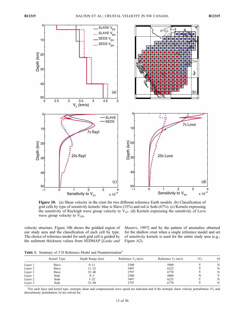
Figure 11. 3‐D seismic model of the study area, determined using the radially anisotropic referencemodel and kernels. (a–c) Isotropic velocity perturbation at 2, 15, and 30 km depth. The white and blacklines indicate the Tintina fault and Great Slave Lake Shear Zone. The white barbed line shows theCordilleran Deformation Front. (d) Sediment thickness in kilometers. The white lines indicate the Bowserand Nechako basins and the 3000 m contour of the Western Canada Sedimentary Basin.


14 of 30

alternative to the linear inversion described here, a modelspace search is an effective approach for placing constraintson and quantifying the uncertainties in a 3‐D Earth model[e.g., Ritzwoller et al., 2004].[38] In matrix notation, equation (10) can be written

G � x ¼ d; ð11Þ

where the vector d contains the data to be fit (i.e., dUi(w)),the vector x contains the unknown coefficients (i.e., dVS

jm

and dd1j), and G relates these two quantities. As in section 5,

we seek a least‐squares solution to equation (11). Weminimize the squared gradient of the isotropic velocityperturbations, as defined in equation (3). This horizontalsmoothness constraint can be implemented as a linear con-straint B · x = c [e.g., Boschi and Dziewonski, 1999], whereB has dimensions 2N × N. Each row of B contains only twonon‐zero elements, corresponding to the jth and jEth cells orto the jth and jSth cells, which have values of 1 and −1,respectively. (See equation (3) for specific notation.) Then,equation (3) can be written as ∥B · x∥ 2, and the linearsystem B · x = 0 can be used. Equation (11) becomes

G�B

� �� x ¼ d

c

� �; ð12Þ

where the strength of the constraint is controlled by dampingcoefficient a, with c = 0. The influence of the choice of aon the model characteristics and misfit is discussed inAppendix A. We do not damp model gradients in the ver-tical direction, as the vertical parameterization is alreadyfairly coarse. A separate horizontal smoothness constraint isapplied to the sedimentary layer thicknesses. The damped,least‐squares solution to equation (12) is

xLS ¼ GT � Gþ �2BT � B� �1� GT � dþ �2BT � c� : ð13Þ

6.4. The 3‐D Model Results

[39] Figures 11a–11d show the model obtained byinverting the Love and Rayleigh wave group velocityobservations using the radially anisotropic reference modelsand their associated kernels as described above. The 7 s, 15 s,and 20 s Rayleigh wave and 7 s, 14 s, and 18 s Love wavedata are inverted (Table 2). These periods were chosen tooptimize depth sensitivity throughout the crust, taking intoconsideration the frequency bands in which the signal‐to‐noise ratio is highest for our data set; longer‐period datahave low SNR and are therefore not included. Sedimentthickness (Figure 11d) is greatest (5–6 km) in the south-eastern portion of the study area and near the center point ofthe CANOE array, in agreement with sediment thickness

values from the Western Canada Sedimentary Basin. In thecells for which the Slave kernels are used, at 2 km depththe highest velocities are found in the northeast corner(3.3–3.4 km/s) with slightly lower velocities in the southwestregion (3.1–3.3 km/s). In the middle crust (Figure 11b; 15 kmdepth), the model contains a zone of low velocity extendingfrom north to south through the western two‐thirds of thestudy area. In general, high velocity at this depth is located inthe eastern section of the area. In the lower crust (Figure 11c;30 km), the model contains a zone of high velocities in thecenter of the study area that extends to the northeast andnorthwest. The remainder of the region is characterized byaverage to low wave speeds, especially west of the Cordil-leran Deformation Front.[40] The misfit between the observations and the model

predictions is summarized in Table 2. We use the goodness‐of‐fit parameter c2/M:

�2

M¼ 1

M

XMj¼1

1

�2j

�Uobsj � �Upred

j

�2; ð14Þ

where the sum is over all observations M, the predictedgroup speed dUj

pred is calculated from the right‐hand‐side ofequation (10), and sj is the observational uncertainty foreach measurement, which we estimate from the standarddeviation of the distribution of group velocities measuredfor similar paths. When the difference between the model‐predicted and the observed group speeds is similar to theobservational uncertainty, c2/M approaches unity. Not sur-prisingly, the 3‐D model provides a slightly worse fit to thedata than the 2‐D maps (Figures 8–9), due to inconsistenciesbetween the data sets at different periods and the need to fitthe Rayleigh and Love waves simultaneously. Table 2contains misfit values for 3‐D models determined onlyfrom the Love wave data and only from the Rayleigh wavedata (Figure A5). These values are very similar to the misfitsfor the 2‐D maps, suggesting that the poorer fit provided bythe 3‐D model primarily reflects difficulties associated withfitting the Rayleigh and Love waves simultaneously.

6.5. Resolution Tests

[41] Figure 12 summarizes a series of resolution tests. Theinput model consists of five rectangular anomalies distrib-uted throughout the study area. This pattern is assigned toeither layer 1, layer 2, or layer 3.When it is assigned to layer 1,uniform velocity is prescribed for layers 2 and 3; when it isassigned to layer 2, uniform velocity is prescribed for layers 1and 3, and so on. Synthetic group velocity is calculated foreach ray path in our data set using equations for the forwardproblem (equation (10)), the sensitivity kernels calculatedfor the Slave reference model, and the velocity structure of

Table 2. Misfit (c2/M) for the Six Group Velocity Data Sets for the 2‐D Maps in Figures 8 and 9 and the 3‐D Model in Figure 11a

7 s Rayleigh 15 s Rayleigh 20 s Rayleigh 7 s Love 14 s Love 18 s Love

N 2776 2701 2534 1887 1690 15953‐D model 2.0 2.3 2.2 1.3 2.8 2.42‐D maps 1.0 0.8 0.7 1.1 0.9 0.93‐D model, Love only 2.1 23.4 12.2 0.9 1.0 1.03‐D model, Rayleigh only 1.0 0.9 0.8 12.6 4.6 4.2

aThe number of observations N is provided in addition to the misfit for 3‐D models derived only from the Love wave data and only from the Rayleighwave data.


15 of 30

Figure

12.

(a)Resultsof

threeresolutio

ntests.The

inputm

odelcontains

five

rectangularanom

alieswith

positiv

evelocity

perturbatio

n(5%).Thispattern

isassigned

toeither

layer1,

layer2,

orlayer3;

ineach

case,theothertwolayers

arepre-

scribeduniform

velocity.The

recoveredmodelsfrom

each

ofthethreeresolutio

ntestsareshow

nin

therightpanels.Geo-

logicfeatures

areas

inFigure1.

(b)Asummaryof

theaveragetotalp

athlength

forallp

aths

passingthrougheach

grid

cell.

Unitsaredegreesof

epicentral

distance

(1°∼111km

).


16 of 30

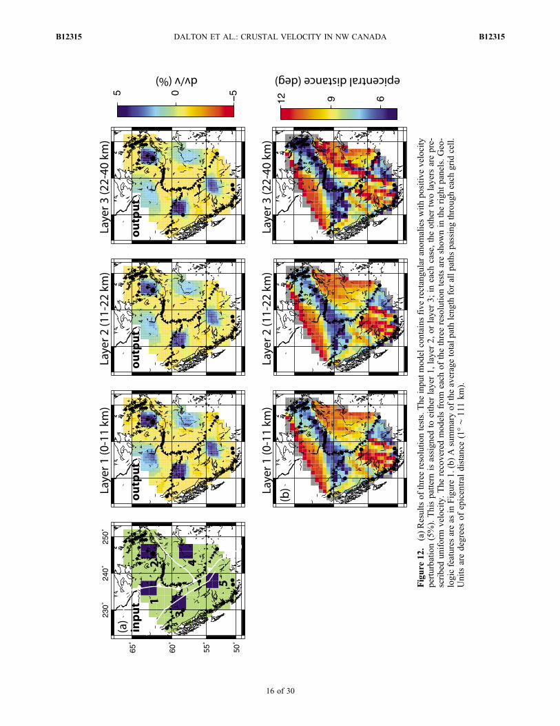
the input model designed for this test. The recovered modelsindicate little vertical smearing of the input anomalies; thus,in Figure 12a, we only present the recovered models for thelayer that was assigned the anomaly pattern (i.e., output forlayer 1 corresponds to the resolution test with inputanomalies only in layer 1). In all three tests, anomalies 2 and3 are recovered nearly perfectly, anomaly 5 is fairly wellrecovered, and anomalies 1 and 4 are less well recovered.[42] The reason for the different levels of success in the

resolution tests is related to the path coverage of the area. Itis clear from Figures 6 and 7 that short paths of length<600 km primarily connect the stations of the CANOE arrayand, to some extent, the POLARIS stations in the northeast.The rest of the study area is sampled by longer paths. InFigure 12b, coverage by paths of different lengths has beenquantified. The study area has been divided into a number ofgrid cells, and we have calculated the average total length ofthe paths that traverse each grid cell. To account for thedepth sensitivities of the Love and Rayleigh waves in our dataset, the average of path lengths summarized in Figure 12bhas been weighted by the integrated sensitivity of eachdata set to each layer (e.g., we have considered the sensi-tivity of 7 s Rayleigh waves to each layer, of 14 s Rayleighwaves to each layer, etc.). The results show that in allthree layers, the northwestern and southeastern regions areprimarily traversed by long paths; accordingly, the inputanomalies in these regions are recovered but are horizon-tally smeared, resulting in a weaker recovered anomaly(Figure 12a). This effect is most clearly observed in layer 3.However, the central and southern sections of the region aresampled by many shorter paths, which enhances the modelresolution and allows the location and amplitude of the inputanomalies to be faithfully recovered.

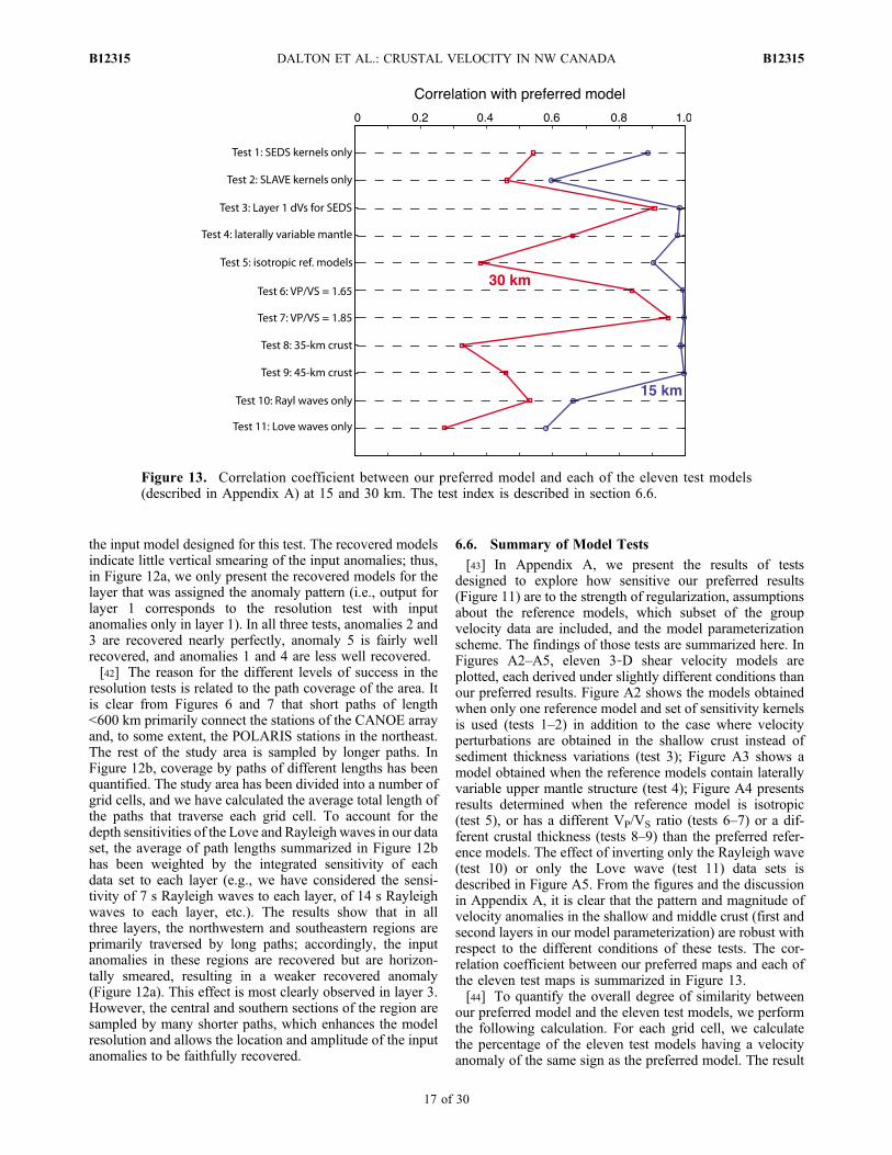
6.6. Summary of Model Tests

[43] In Appendix A, we present the results of testsdesigned to explore how sensitive our preferred results(Figure 11) are to the strength of regularization, assumptionsabout the reference models, which subset of the groupvelocity data are included, and the model parameterizationscheme. The findings of those tests are summarized here. InFigures A2–A5, eleven 3‐D shear velocity models areplotted, each derived under slightly different conditions thanour preferred results. Figure A2 shows the models obtainedwhen only one reference model and set of sensitivity kernelsis used (tests 1–2) in addition to the case where velocityperturbations are obtained in the shallow crust instead ofsediment thickness variations (test 3); Figure A3 shows amodel obtained when the reference models contain laterallyvariable upper mantle structure (test 4); Figure A4 presentsresults determined when the reference model is isotropic(test 5), or has a different VP/VS ratio (tests 6–7) or a dif-ferent crustal thickness (tests 8–9) than the preferred refer-ence models. The effect of inverting only the Rayleigh wave(test 10) or only the Love wave (test 11) data sets isdescribed in Figure A5. From the figures and the discussionin Appendix A, it is clear that the pattern and magnitude ofvelocity anomalies in the shallow and middle crust (first andsecond layers in our model parameterization) are robust withrespect to the different conditions of these tests. The cor-relation coefficient between our preferred maps and each ofthe eleven test maps is summarized in Figure 13.[44] To quantify the overall degree of similarity between

our preferred model and the eleven test models, we performthe following calculation. For each grid cell, we calculatethe percentage of the eleven test models having a velocityanomaly of the same sign as the preferred model. The result

Figure 13. Correlation coefficient between our preferred model and each of the eleven test models(described in Appendix A) at 15 and 30 km. The test index is described in section 6.6.


17 of 30

(Figure A6) provides a measure of the degree of consistencyof high‐ and low‐velocity features between models. We findthat the preferred model at 15 km depth is remarkablyrobust: for almost all of the grid cells, 90–100% of themodels tested show a consistent sign of velocity anomaly.This suggests that the structure through the upper andmiddle crust can be interpreted with a high degree of con-fidence. In the bottom layer (30 km depth), agreementbetween models is weaker; the velocity perturbations inthe central portion of the study area are robust, but outsidethe center region, the nature of the perturbation depends onthe assumptions of the inversion. This is because our datahave relatively low sensitivity to this layer; it is also becausethe velocity of this layer trades off with crustal thickness andupper mantle structure. As a result, in the discussion thatfollows, we limit our interpretation of the lower crustalvelocities to the central, well‐constrained portion of theregion.

7. Discussion

[45] In the upper mantle, temperature is the primary causeof perturbations in wave speed at a fixed depth; variability inrock and mineral composition has a smaller effect [e.g., Lee,2003; Shapiro and Ritzwoller, 2004; Faul and Jackson,2005]. Recent seismic images of the upper mantle acrossnorthwestern Canada have been obtained from teleseismicbody waves [e.g., Mercier et al., 2008, 2009] and surfacewaves [Frederiksen et al., 2001; van der Lee and Frederiksen,2005; Nettles and Dziewonski, 2008]. These studies suggestthat the upper mantle structure is dominated by a substantialtemperature contrast between the high‐temperature, tectoni-cally young Cordillera and the lower‐temperature ancientcraton; the boundary between these upper mantle domainsroughly corresponds to the deformation front (Figure 15).[46] The crust, on the other hand, is a highly heteroge-

neous collage of different rock and mineral types that, whenconsidered together with laterally variable thermal condi-tions, makes it difficult to uniquely interpret crustal seismicvelocities [e.g., Christensen and Mooney, 1995]. This isespecially true in our study area, which includes cratons,

ancient and recent orogens, former magmatic arcs, episodesof extension, and thick sediment basins. Our images ofcrustal velocity (Figure 11) are different than the mantleimages (Figure 15) in that they do not show a strong contrastacross the deformation front that can be interpreted in termsof temperature. To gain a better understanding of themechanisms that control crustal velocities in this region, weanalyze our 3‐D model with earlier results from theLithoprobe program, specifically the Slave‐Northern Cor-dillera Lithosphere Evolution (SNORCLE) project [e.g.,Cook and Erdmer, 2005]. The SNORCLE transects consistof seismic reflection and refraction data acquired along fourlines (Figure 1b). Detailed point and/or linear constraintsobtained from the SNORCLE data allow us to develop amore robust interpretation of lateral variations of shearvelocity structure in the region.

7.1. The 3‐D Crustal Velocity Structure

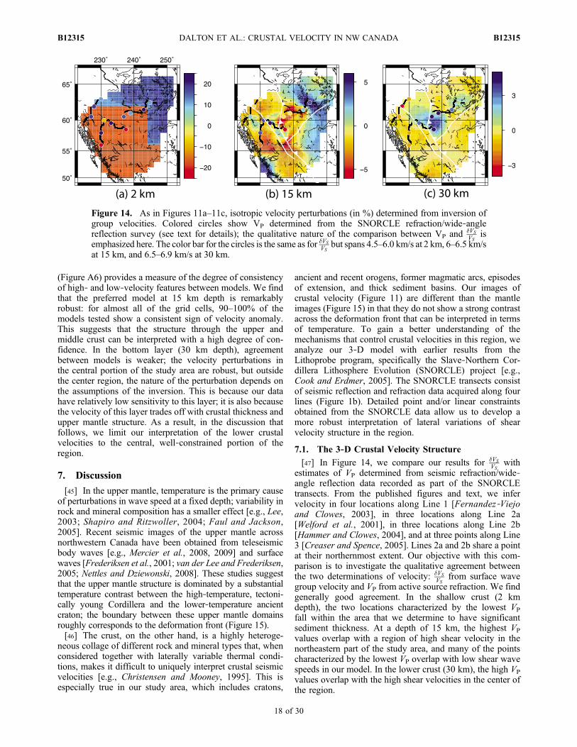
[47] In Figure 14, we compare our results for �VSVS

withestimates of VP determined from seismic refraction/wide‐angle reflection data recorded as part of the SNORCLEtransects. From the published figures and text, we infervelocity in four locations along Line 1 [Fernandez‐Viejoand Clowes, 2003], in three locations along Line 2a[Welford et al., 2001], in three locations along Line 2b[Hammer and Clowes, 2004], and at three points along Line3 [Creaser and Spence, 2005]. Lines 2a and 2b share a pointat their northernmost extent. Our objective with this com-parison is to investigate the qualitative agreement betweenthe two determinations of velocity: �VS

VSfrom surface wave

group velocity and VP from active source refraction. We findgenerally good agreement. In the shallow crust (2 kmdepth), the two locations characterized by the lowest VP

fall within the area that we determine to have significantsediment thickness. At a depth of 15 km, the highest VP

values overlap with a region of high shear velocity in thenortheastern part of the study area, and many of the pointscharacterized by the lowest VP overlap with low shear wavespeeds in our model. In the lower crust (30 km), the high VP

values overlap with the high shear velocities in the center ofthe region.

Figure 14. As in Figures 11a–11c, isotropic velocity perturbations (in %) determined from inversion ofgroup velocities. Colored circles show VP determined from the SNORCLE refraction/wide‐anglereflection survey (see text for details); the qualitative nature of the comparison between VP and �VS

VSis

emphasized here. The color bar for the circles is the same as for �VSVS

but spans 4.5–6.0 km/s at 2 km, 6–6.5 km/sat 15 km, and 6.5–6.9 km/s at 30 km.


18 of 30

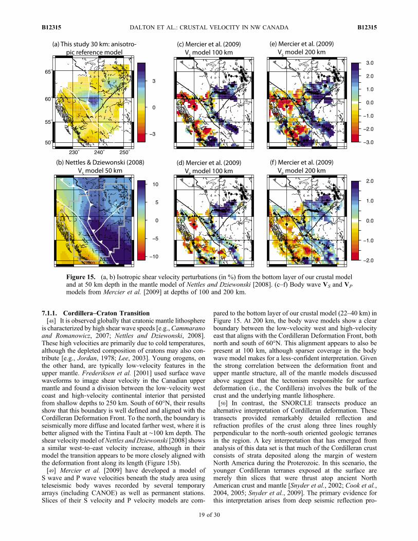
7.1.1. Cordillera–Craton Transition[48] It is observed globally that cratonic mantle lithosphere

is characterized by high shear wave speeds [e.g.,Cammaranoand Romanowicz, 2007; Nettles and Dziewonski, 2008].These high velocities are primarily due to cold temperatures,although the depleted composition of cratons may also con-tribute [e.g., Jordan, 1978; Lee, 2003]. Young orogens, onthe other hand, are typically low‐velocity features in theupper mantle. Frederiksen et al. [2001] used surface wavewaveforms to image shear velocity in the Canadian uppermantle and found a division between the low‐velocity westcoast and high‐velocity continental interior that persistedfrom shallow depths to 250 km. South of 60°N, their resultsshow that this boundary is well defined and aligned with theCordilleran Deformation Front. To the north, the boundary isseismically more diffuse and located farther west, where it isbetter aligned with the Tintina Fault at ∼100 km depth. Theshear velocity model ofNettles and Dziewonski [2008] showsa similar west‐to‐east velocity increase, although in theirmodel the transition appears to be more closely aligned withthe deformation front along its length (Figure 15b).[49] Mercier et al. [2009] have developed a model of

S wave and P wave velocities beneath the study area usingteleseismic body waves recorded by several temporaryarrays (including CANOE) as well as permanent stations.Slices of their S velocity and P velocity models are com-

pared to the bottom layer of our crustal model (22–40 km) inFigure 15. At 200 km, the body wave models show a clearboundary between the low‐velocity west and high‐velocityeast that aligns with the Cordilleran Deformation Front, bothnorth and south of 60°N. This alignment appears to also bepresent at 100 km, although sparser coverage in the bodywave model makes for a less‐confident interpretation. Giventhe strong correlation between the deformation front andupper mantle structure, all of the mantle models discussedabove suggest that the tectonism responsible for surfacedeformation (i.e., the Cordillera) involves the bulk of thecrust and the underlying mantle lithosphere.[50] In contrast, the SNORCLE transects produce an

alternative interpretation of Cordilleran deformation. Thesetransects provided remarkably detailed reflection andrefraction profiles of the crust along three lines roughlyperpendicular to the north‐south oriented geologic terranesin the region. A key interpretation that has emerged fromanalysis of this data set is that much of the Cordilleran crustconsists of strata deposited along the margin of westernNorth America during the Proterozoic. In this scenario, theyounger Cordilleran terranes exposed at the surface aremerely thin slices that were thrust atop ancient NorthAmerican crust and mantle [Snyder et al., 2002; Cook et al.,2004, 2005; Snyder et al., 2009]. The primary evidence forthis interpretation arises from deep seismic reflection pro-

Figure 15. (a, b) Isotropic shear velocity perturbations (in %) from the bottom layer of our crustal modeland at 50 km depth in the mantle model of Nettles and Dziewonski [2008]. (c–f) Body wave VS and VP

models from Mercier et al. [2009] at depths of 100 and 200 km.


19 of 30

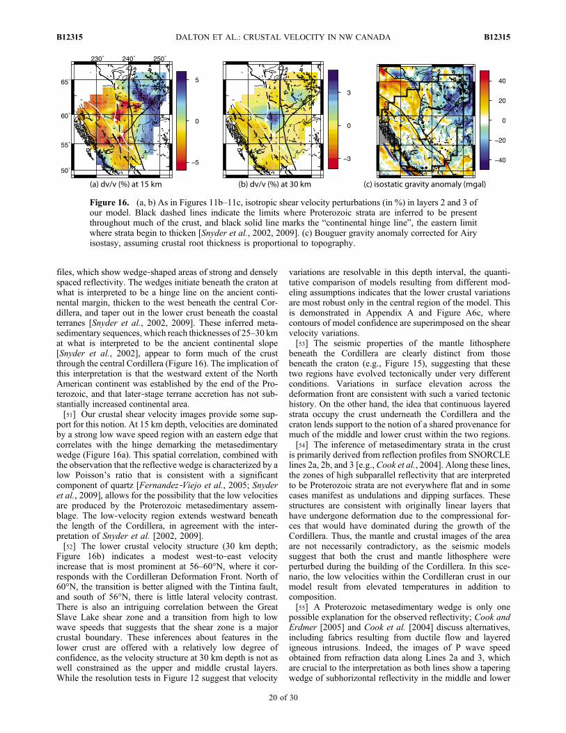
files, which show wedge‐shaped areas of strong and denselyspaced reflectivity. The wedges initiate beneath the craton atwhat is interpreted to be a hinge line on the ancient conti-nental margin, thicken to the west beneath the central Cor-dillera, and taper out in the lower crust beneath the coastalterranes [Snyder et al., 2002, 2009]. These inferred meta-sedimentary sequences, which reach thicknesses of 25–30 kmat what is interpreted to be the ancient continental slope[Snyder et al., 2002], appear to form much of the crustthrough the central Cordillera (Figure 16). The implication ofthis interpretation is that the westward extent of the NorthAmerican continent was established by the end of the Pro-terozoic, and that later‐stage terrane accretion has not sub-stantially increased continental area.[51] Our crustal shear velocity images provide some sup-

port for this notion. At 15 km depth, velocities are dominatedby a strong low wave speed region with an eastern edge thatcorrelates with the hinge demarking the metasedimentarywedge (Figure 16a). This spatial correlation, combined withthe observation that the reflective wedge is characterized by alow Poisson’s ratio that is consistent with a significantcomponent of quartz [Fernandez‐Viejo et al., 2005; Snyderet al., 2009], allows for the possibility that the low velocitiesare produced by the Proterozoic metasedimentary assem-blage. The low‐velocity region extends westward beneaththe length of the Cordillera, in agreement with the inter-pretation of Snyder et al. [2002, 2009].[52] The lower crustal velocity structure (30 km depth;

Figure 16b) indicates a modest west‐to‐east velocityincrease that is most prominent at 56–60°N, where it cor-responds with the Cordilleran Deformation Front. North of60°N, the transition is better aligned with the Tintina fault,and south of 56°N, there is little lateral velocity contrast.There is also an intriguing correlation between the GreatSlave Lake shear zone and a transition from high to lowwave speeds that suggests that the shear zone is a majorcrustal boundary. These inferences about features in thelower crust are offered with a relatively low degree ofconfidence, as the velocity structure at 30 km depth is not aswell constrained as the upper and middle crustal layers.While the resolution tests in Figure 12 suggest that velocity

variations are resolvable in this depth interval, the quanti-tative comparison of models resulting from different mod-eling assumptions indicates that the lower crustal variationsare most robust only in the central region of the model. Thisis demonstrated in Appendix A and Figure A6c, wherecontours of model confidence are superimposed on the shearvelocity variations.[53] The seismic properties of the mantle lithosphere

beneath the Cordillera are clearly distinct from thosebeneath the craton (e.g., Figure 15), suggesting that thesetwo regions have evolved tectonically under very differentconditions. Variations in surface elevation across thedeformation front are consistent with such a varied tectonichistory. On the other hand, the idea that continuous layeredstrata occupy the crust underneath the Cordillera and thecraton lends support to the notion of a shared provenance formuch of the middle and lower crust within the two regions.[54] The inference of metasedimentary strata in the crust

is primarily derived from reflection profiles from SNORCLElines 2a, 2b, and 3 [e.g., Cook et al., 2004]. Along these lines,the zones of high subparallel reflectivity that are interpretedto be Proterozoic strata are not everywhere flat and in somecases manifest as undulations and dipping surfaces. Thesestructures are consistent with originally linear layers thathave undergone deformation due to the compressional for-ces that would have dominated during the growth of theCordillera. Thus, the mantle and crustal images of the areaare not necessarily contradictory, as the seismic modelssuggest that both the crust and mantle lithosphere wereperturbed during the building of the Cordillera. In this sce-nario, the low velocities within the Cordilleran crust in ourmodel result from elevated temperatures in addition tocomposition.[55] A Proterozoic metasedimentary wedge is only one

possible explanation for the observed reflectivity; Cook andErdmer [2005] and Cook et al. [2004] discuss alternatives,including fabrics resulting from ductile flow and layeredigneous intrusions. Indeed, the images of P wave speedobtained from refraction data along Lines 2a and 3, whichare crucial to the interpretation as both lines show a taperingwedge of subhorizontal reflectivity in the middle and lower

Figure 16. (a, b) As in Figures 11b–11c, isotropic shear velocity perturbations (in %) in layers 2 and 3 ofour model. Black dashed lines indicate the limits where Proterozoic strata are inferred to be presentthroughout much of the crust, and black solid line marks the “continental hinge line”, the eastern limitwhere strata begin to thicken [Snyder et al., 2002, 2009]. (c) Bouguer gravity anomaly corrected for Airyisostasy, assuming crustal root thickness is proportional to topography.


20 of 30

crust, do not contain a velocity contrast corresponding to theboundaries of this wedge [Hammer and Clowes, 2004;Creaser and Spence, 2005]. This does not rule out thepresence of metasedimentary strata in the crust, but it doesrequire that adjacent but disparate tectonic terranes havevery similar compressional wave velocities. While thisinconclusive result from the refraction data would seem toweaken the case for a metasedimentary wedge, we note thatwhen S wave velocities measured from the same two linesare also considered, a wedge‐shaped region of low VP/VS

that corresponds spatially with the reflectivity zones isobtained [Fernandez‐Viejo et al., 2005].7.1.2. Archean‐Proterozoic Transition[56] The combination of the CANOE A leg and

POLARIS stations provides good resolution of crustalstructure across the transition from the Archean Slave cratoninto the Proterozoic terranes to the west (Figure 1). At bothmidcrustal (15 km) and lower crustal (30 km) depths, partsof the Slave craton are characterized by lower velocities thanthe adjacent Proterozoic crust to the west, although thelower crustal transition cannot be interpreted with highconfidence. (Figure A6c shows contours of model confi-dence superimposed on lower crustal velocity structure.)Both are consistent with P wave velocities observed in themiddle and lower crust along SNORCLE Line 1[Fernandez‐Viejo and Clowes, 2003], which show lowerwave speed beneath the Archean Contwoyto terrane andhigher velocity under the Anton terrane and ProterozoicGreat Bear arc to the west. A zone of low P wave speedsbeneath the Hottah terrane [Fernandez‐Viejo and Clowes,2003] corresponds spatially with the gap that separates thetwo high‐velocity anomalies at 30 km depth in our model(Figure 16b).[57] Low VP/VS values throughout the Slave craton crust

along SNORCLE Line 1 have been identified byFernandez‐Viejo et al. [2005] and, together with the VP

results mentioned above, are attributed to a silica‐richcomposition. At the westward transition from Slave cratonto Wopmay orogen, VP/VS values increase, suggesting amore mafic crust. Increasing SiO2 content leads to lowercompressional wave speeds and Poisson’s ratios in manycommon crustal rock types [Christensen, 1996; Rudnick and

Fountain, 1995]. Our results are also consistent with globalaverage VP values for Archean lower crust, which are 0.1–0.2 km/s lower than for Proterozoic shields (although thevalues overlap within uncertainty) [Rudnick and Fountain,1995]. It also may be consistent with weakening associ-ated with metasomatism and kimberlite volcanism over thelong history of the craton. Either way, it is suggestive of adistinctive history for the Archean portion of the craton,relative to the Proterozoic portion.

7.2. Crustal Thickness

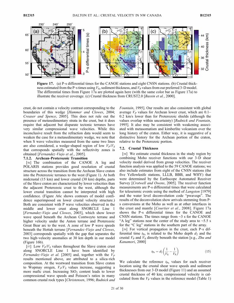
[58] We estimate crustal thickness in the study region bycombining Moho receiver functions with our 3‐D shearvelocity model derived from group velocities. The receiverfunction analysis was applied to the 59 CANOE stations; wealso include estimates from eight of the CNSN stations (thefive Yellowknife stations, LLLB, BBB, and WHY) thatwere determined by the Earthscope Automated ReceiverSurvey [Crotwell and Owens, 2005]. The receiver functionmeasurements are P‐s differential times that were calculatedfor teleseismic events using the method of Langston [1979]and the water level deconvolution code “pwaveqn”. Theresults of the deconvolution show arrivals stemming from P‐s conversions at the Moho as well as at other interfaces inthe crust and mantle [Courtier et al., 2008]. Figure 17ashows the P‐s differential times for the CANOE andCNSN stations. The times range from ∼3 s for the CANOE“A leg” stations near the center of the study area to ∼5.5 sfor the “C leg” stations in the southern part of the array.[59] For vertical propagation in the crust, each P‐s dif-

ferential time tPs is related to the Moho depth d2 and thecrustal VP and VS directly beneath the station [e.g., Zhu andKanamori, 2000]

tPs ¼ d21

VS� 1

VP

� �ð15Þ

We calculate the reference tPs values for each receiverlocation using the crustal shear wave speeds and sedimentthicknesses from our 3‐D model (Figure 11) and an assumedcrustal thickness of 40 km; compressional velocity is cal-culated from the VP values in the reference model (Table 1)

Figure 17. (a) P‐s differential times for the CANOE stations and eight CNSN stations. (b) Crustal thick-ness estimated from the P‐s times usingVS, sediment thickness, andVP values from our preferred 3‐Dmodel.The differential times from Figure 17a are plotted again here (with the same color bar as Figure 17a) toillustrate the receiver coverage. (c) Crustal thickness from CRUST2.0 [Bassin et al., 2000].


21 of 30

and the assumed scaling dVP = kdVS (section 6.1). Thereference times are subtracted from the measured P‐s dif-ferential times, resulting in the anomaly dtPs that is related toperturbations in shear velocity dVS, compressional velocitydVP, and Moho depth dd2 by

�tPs ¼ � d2V 2S

�VS þ d2V 2P

�VP þ �d21

VS� 1

VP

� �: ð16Þ

We assume that the perturbations in velocity structure arewell constrained by the inversion of group speeds andattribute each dtPs value to perturbations Moho depth. ThedtPs values are then inverted for lateral variations in dd2, andwe apply a horizontal smoothness constraint to the Mohoperturbations.[60] The resulting map of Moho depths (Figure 17b)

largely mirrors the pattern of P‐s differential time mea-surements, with the thinnest crust (∼34–36 km) in the centerand northwestern corner of the study area and slightlythicker crust (∼38–42 km) to the south and east. The Mohodepths in Figure 17b provide a good fit to the measureddifferential times; the median absolute value of the residualbetween observed and predicted tPs is 0.12 s. Observationaluncertainty s of the receiver function times can be estimatedfrom the standard deviation of the five Yellowknife stations,which are nearly colocated, to be 0.22 s. Applying this valueto all of the differential time measurements yields c2/M =1.05 for the receiver function data set; smaller values of swould increase the c2/M estimate.[61] The absolute Moho depths obtained from the P‐s

differential times are dependent on the assumed VP/VS ratio.With VP/VS = 1.65, Moho depths are ∼5 km larger than inFigure 17b, and with VP/VS = 1.85 they are ∼5 km smaller.However, the pattern of crustal thickness variations is notaffected by these assumptions; correlation coefficientbetween all pairs of maps is >0.99. Laterally variable VP/VS

ratios will also affect the retrieved Moho depths. Our dataare not able to constrain variations in VP/VS, but the rangeof 1.65–1.85 tested here is larger than expected for typicalcrustal rocks [e.g., Christensen, 1996]. The results in Figure17b are not affected by the crustal thickness of the referencemodel; we obtain nearly identical patterns and absolutevalues of Moho depth for reference models with 35 km,40 km, and 45 km crustal thickness. Crustal thickness valuesfrom CRUST2.0 (Figure 17c) [Bassin et al., 2000] alsoshow the thickest crust in the southeastern corner, whichthins to the northwest along the deformation front.[62] The overall pattern of crustal thickness roughly cor-

relates with large‐scale tectonics: thinner crust beneath theCordillera, and thicker crust beneath the craton. This isopposite to the pattern expected for an Airy isostaticmechanism, wherein a thick crustal root is expected tocompensate for topographic loads at the surface. Variationsin crustal thickness along the Cordillera generally agree withisostatic gravity anomalies calculated for the study area(Natural Resources Canada, Geoscience Data Repository).Isostatic gravity was calculated using an Airy‐Heiskanenmodel, where the depth of crustal roots is proportional to thesurface elevation scaled by an assumed density contrastbetween the crustal root and mantle. The Bouguer gravityanomaly is then corrected for the gravity signal associatedwith this assumed crustal root, and non‐zero isostatic

gravity values identify locations where the assumption ofroot thickness or density contrast was incorrect; theanomalies could also result from heterogeneity in the man-tle. North of 57°N, isostatic gravity is mostly high along theCordillera (Figure 16c), possibly reflecting anomalouslythin crust.

8. Conclusions

[63] We computed cross correlations of day long timeseries of ambient noise at 99 broadband seismic stationslocated in northwestern Canada for the time period July2004 to June 2005. The stacked cross correlations yieldedsufficiently high signal‐to‐noise ratios at all interstationazimuths, although SNR is especially strong in the azimuthband 20°–110°, roughly perpendicular to the Pacific coast-line. Furthermore, the causal and anticausal sides of thecross correlations are not of equal strength for the intersta-tion azimuth band 0°–100°, suggesting a high level ofcoherent noise propagation to the northeast and weakercoherent noise propagation in other directions.[64] Group velocity as a function of frequency is mea-

sured from the vertical component and transverse compo-nent ambient noise cross correlations. Strong regional trendsare clear in the group velocity dispersion curves (e.g.,Figure 5), with paths characterized by higher than averagevelocity at all periods clustering in the northeastern corner ofthe study area and paths that are slower than average at allperiods concentrated in the center of the study area. Pathswith high velocity at short periods and lower wave speed atlong periods mostly traverse the north central section,whereas paths characterized by slow velocity at short peri-ods and fast wave speed at longer periods predominantlycross east of the center of the study area.[65] These Rayleigh and Love wave group velocity

observations are inverted for 3‐D shear velocity structure.We allow for locally variable sensitivity kernels, sinceportions of the study area are covered in several kilometersof sedimentary rock while other portions are devoid ofsediments. We fix radial anisotropy in the middle and lowercrust, with VSH > VSV by 0.2 km/s, but do not allow forlateral variations in anisotropy.[66] Near the surface, the largest sediment thickness

values (4–5 km) retrieved from the joint inversion of groupvelocity and receiver function data overlap in location withknown sedimentary basins (Western Canada SedimentaryBasin, Bower Basin, Nechako Basin). In the middle crust,much of the region west of Great Slave Lake is character-ized by low wave speeds. The easternmost extent of thisslow‐velocity region coincides with the ancient continentalmargin inferred from SNORCLE active source reflectionstudies [e.g., Snyder et al., 2009], and the low wave speedsare consistent with the interpretation of Proterozoic meta-sedimentary strata in the middle and lower crust beneath theCordillera. In this scenario, many of the Cordilleran terranesare thin flakes thrust atop these older rocks, which arehypothesized to have originated as sediments deposited in apassive margin setting.[67] Images of the upper mantle beneath the study area

provide convincing evidence for a strong temperature con-trast between the warmer Cordillera and cooler continentalinterior; the shear velocity anomalies in the lower crust of


22 of 30

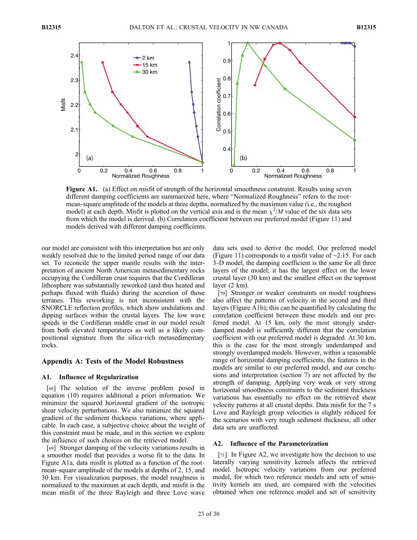
our model are consistent with this interpretation but are onlyweakly resolved due to the limited period range of our dataset. To reconcile the upper mantle results with the inter-pretation of ancient North American metasedimentary rocksoccupying the Cordilleran crust requires that the Cordilleranlithosphere was substantially reworked (and thus heated andperhaps fluxed with fluids) during the accretion of thoseterranes. This reworking is not inconsistent with theSNORCLE reflection profiles, which show undulations anddipping surfaces within the crustal layers. The low wavespeeds in the Cordilleran middle crust in our model resultfrom both elevated temperatures as well as a likely com-positional signature from the silica‐rich metasedimentaryrocks.

Appendix A: Tests of the Model Robustness

A1. Influence of Regularization

[68] The solution of the inverse problem posed inequation (10) requires additional a priori information. Weminimize the squared horizontal gradient of the isotropicshear velocity perturbations. We also minimize the squaredgradient of the sediment thickness variations, where appli-cable. In each case, a subjective choice about the weight ofthis constraint must be made, and in this section we explorethe influence of such choices on the retrieved model.[69] Stronger damping of the velocity variations results in

a smoother model that provides a worse fit to the data. InFigure A1a, data misfit is plotted as a function of the root‐mean‐square amplitude of the models at depths of 2, 15, and30 km. For visualization purposes, the model roughness isnormalized to the maximum at each depth, and misfit is themean misfit of the three Rayleigh and three Love wave

data sets used to derive the model. Our preferred model(Figure 11) corresponds to a misfit value of ∼2.15. For each3‐D model, the damping coefficient is the same for all threelayers of the model; it has the largest effect on the lowercrustal layer (30 km) and the smallest effect on the topmostlayer (2 km).[70] Stronger or weaker constraints on model roughness

also affect the patterns of velocity in the second and thirdlayers (Figure A1b); this can be quantified by calculating thecorrelation coefficient between these models and our pre-ferred model. At 15 km, only the most strongly under-damped model is sufficiently different that the correlationcoefficient with our preferred model is degraded. At 30 km,this is the case for the most strongly underdamped andstrongly overdamped models. However, within a reasonablerange of horizontal damping coefficients, the features in themodels are similar to our preferred model, and our conclu-sions and interpretation (section 7) are not affected by thestrength of damping. Applying very weak or very stronghorizontal smoothness constraints to the sediment thicknessvariations has essentially no effect on the retrieved shearvelocity patterns at all crustal depths. Data misfit for the 7 sLove and Rayleigh group velocities is slightly reduced forthe scenarios with very rough sediment thickness; all otherdata sets are unaffected.

A2. Influence of the Parameterization

[71] In Figure A2, we investigate how the decision to uselaterally varying sensitivity kernels affects the retrievedmodel. Isotropic velocity variations from our preferredmodel, for which two reference models and sets of sensi-tivity kernels are used, are compared with the velocitiesobtained when one reference model and set of sensitivity

Figure A1. (a) Effect on misfit of strength of the horizontal smoothness constraint. Results using sevendifferent damping coefficients are summarized here, where “Normalized Roughness” refers to the root‐mean‐square amplitude of the models at three depths, normalized by the maximum value (i.e., the roughestmodel) at each depth. Misfit is plotted on the vertical axis and is the mean c2/M value of the six data setsfrom which the model is derived. (b) Correlation coefficient between our preferred model (Figure 11) andmodels derived with different damping coefficients.


23 of 30

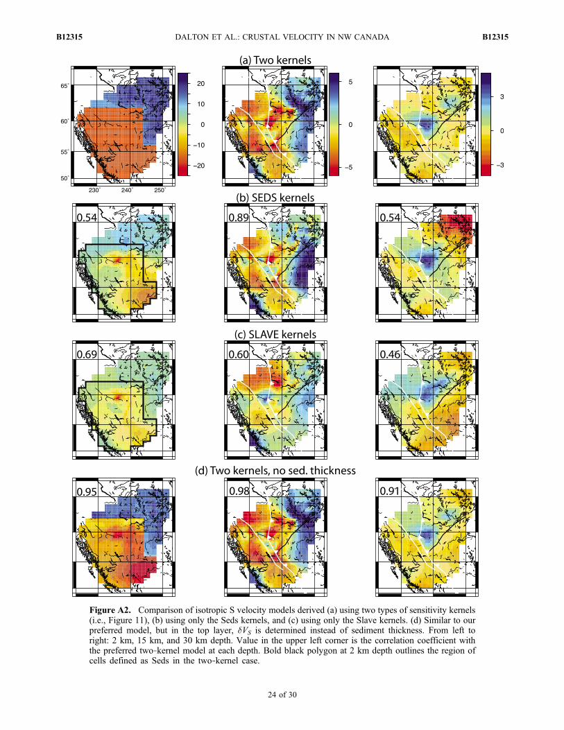
Figure A2. Comparison of isotropic S velocity models derived (a) using two types of sensitivity kernels(i.e., Figure 11), (b) using only the Seds kernels, and (c) using only the Slave kernels. (d) Similar to ourpreferred model, but in the top layer, dVS is determined instead of sediment thickness. From left toright: 2 km, 15 km, and 30 km depth. Value in the upper left corner is the correlation coefficient withthe preferred two‐kernel model at each depth. Bold black polygon at 2 km depth outlines the region ofcells defined as Seds in the two‐kernel case.


24 of 30

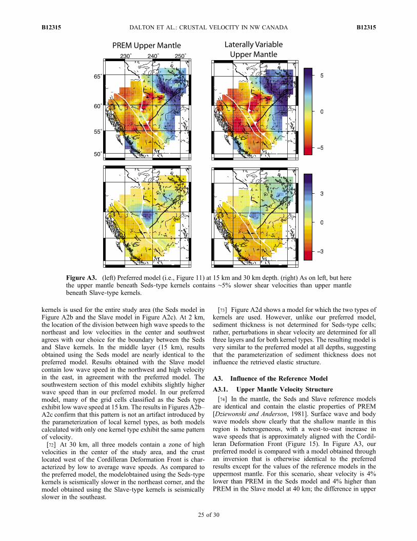
kernels is used for the entire study area (the Seds model inFigure A2b and the Slave model in Figure A2c). At 2 km,the location of the division between high wave speeds to thenortheast and low velocities in the center and southwestagrees with our choice for the boundary between the Sedsand Slave kernels. In the middle layer (15 km), resultsobtained using the Seds model are nearly identical to thepreferred model. Results obtained with the Slave modelcontain low wave speed in the northwest and high velocityin the east, in agreement with the preferred model. Thesouthwestern section of this model exhibits slightly higherwave speed than in our preferred model. In our preferredmodel, many of the grid cells classified as the Seds typeexhibit lowwave speed at 15 km. The results in Figures A2b–A2c confirm that this pattern is not an artifact introduced bythe parameterization of local kernel types, as both modelscalculated with only one kernel type exhibit the same patternof velocity.[72] At 30 km, all three models contain a zone of high

velocities in the center of the study area, and the crustlocated west of the Cordilleran Deformation Front is char-acterized by low to average wave speeds. As compared tothe preferred model, the modelobtained using the Seds‐typekernels is seismically slower in the northeast corner, and themodel obtained using the Slave‐type kernels is seismicallyslower in the southeast.

[73] Figure A2d shows a model for which the two types ofkernels are used. However, unlike our preferred model,sediment thickness is not determined for Seds‐type cells;rather, perturbations in shear velocity are determined for allthree layers and for both kernel types. The resulting model isvery similar to the preferred model at all depths, suggestingthat the parameterization of sediment thickness does notinfluence the retrieved elastic structure.

A3. Influence of the Reference Model

A3.1. Upper Mantle Velocity Structure

[74] In the mantle, the Seds and Slave reference modelsare identical and contain the elastic properties of PREM[Dziewonski and Anderson, 1981]. Surface wave and bodywave models show clearly that the shallow mantle in thisregion is heterogeneous, with a west‐to‐east increase inwave speeds that is approximately aligned with the Cordil-leran Deformation Front (Figure 15). In Figure A3, ourpreferred model is compared with a model obtained throughan inversion that is otherwise identical to the preferredresults except for the values of the reference models in theuppermost mantle. For this scenario, shear velocity is 4%lower than PREM in the Seds model and 4% higher thanPREM in the Slave model at 40 km; the difference in upper

Figure A3. (left) Preferred model (i.e., Figure 11) at 15 km and 30 km depth. (right) As on left, but herethe upper mantle beneath Seds‐type kernels contains ∼5% slower shear velocities than upper mantlebeneath Slave‐type kernels.


25 of 30

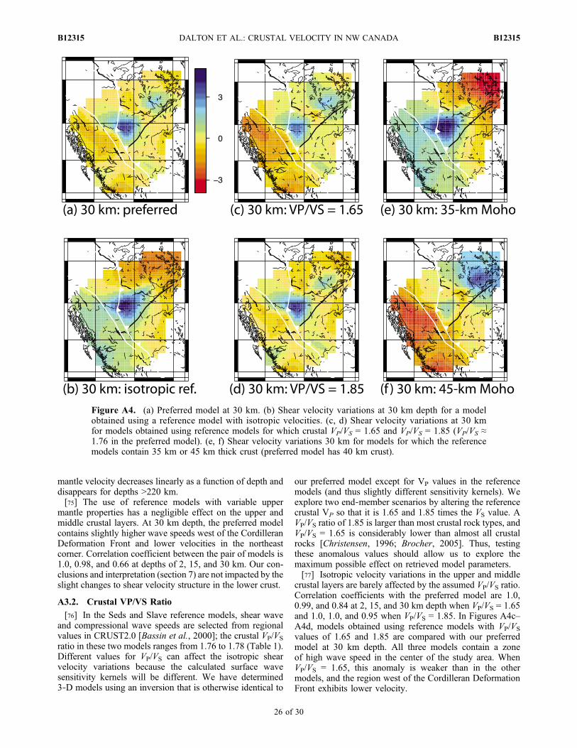
mantle velocity decreases linearly as a function of depth anddisappears for depths >220 km.[75] The use of reference models with variable upper

mantle properties has a negligible effect on the upper andmiddle crustal layers. At 30 km depth, the preferred modelcontains slightly higher wave speeds west of the CordilleranDeformation Front and lower velocities in the northeastcorner. Correlation coefficient between the pair of models is1.0, 0.98, and 0.66 at depths of 2, 15, and 30 km. Our con-clusions and interpretation (section 7) are not impacted by theslight changes to shear velocity structure in the lower crust.

A3.2. Crustal VP/VS Ratio

[76] In the Seds and Slave reference models, shear waveand compressional wave speeds are selected from regionalvalues in CRUST2.0 [Bassin et al., 2000]; the crustal VP/VS

ratio in these two models ranges from 1.76 to 1.78 (Table 1).Different values for VP/VS can affect the isotropic shearvelocity variations because the calculated surface wavesensitivity kernels will be different. We have determined3‐D models using an inversion that is otherwise identical to

our preferred model except for VP values in the referencemodels (and thus slightly different sensitivity kernels). Weexplore two end‐member scenarios by altering the referencecrustal VP so that it is 1.65 and 1.85 times the VS value. AVP/VS ratio of 1.85 is larger than most crustal rock types, andVP/VS = 1.65 is considerably lower than almost all crustalrocks [Christensen, 1996; Brocher, 2005]. Thus, testingthese anomalous values should allow us to explore themaximum possible effect on retrieved model parameters.[77] Isotropic velocity variations in the upper and middle

crustal layers are barely affected by the assumed VP/VS ratio.Correlation coefficients with the preferred model are 1.0,0.99, and 0.84 at 2, 15, and 30 km depth when VP/VS = 1.65and 1.0, 1.0, and 0.95 when VP/VS = 1.85. In Figures A4c–A4d, models obtained using reference models with VP/VS

values of 1.65 and 1.85 are compared with our preferredmodel at 30 km depth. All three models contain a zoneof high wave speed in the center of the study area. WhenVP/VS = 1.65, this anomaly is weaker than in the othermodels, and the region west of the Cordilleran DeformationFront exhibits lower velocity.

Figure A4. (a) Preferred model at 30 km. (b) Shear velocity variations at 30 km depth for a modelobtained using a reference model with isotropic velocities. (c, d) Shear velocity variations at 30 kmfor models obtained using reference models for which crustal VP/VS = 1.65 and VP/VS = 1.85 (VP/VS ≈1.76 in the preferred model). (e, f) Shear velocity variations 30 km for models for which the referencemodels contain 35 km or 45 km thick crust (preferred model has 40 km crust).


26 of 30

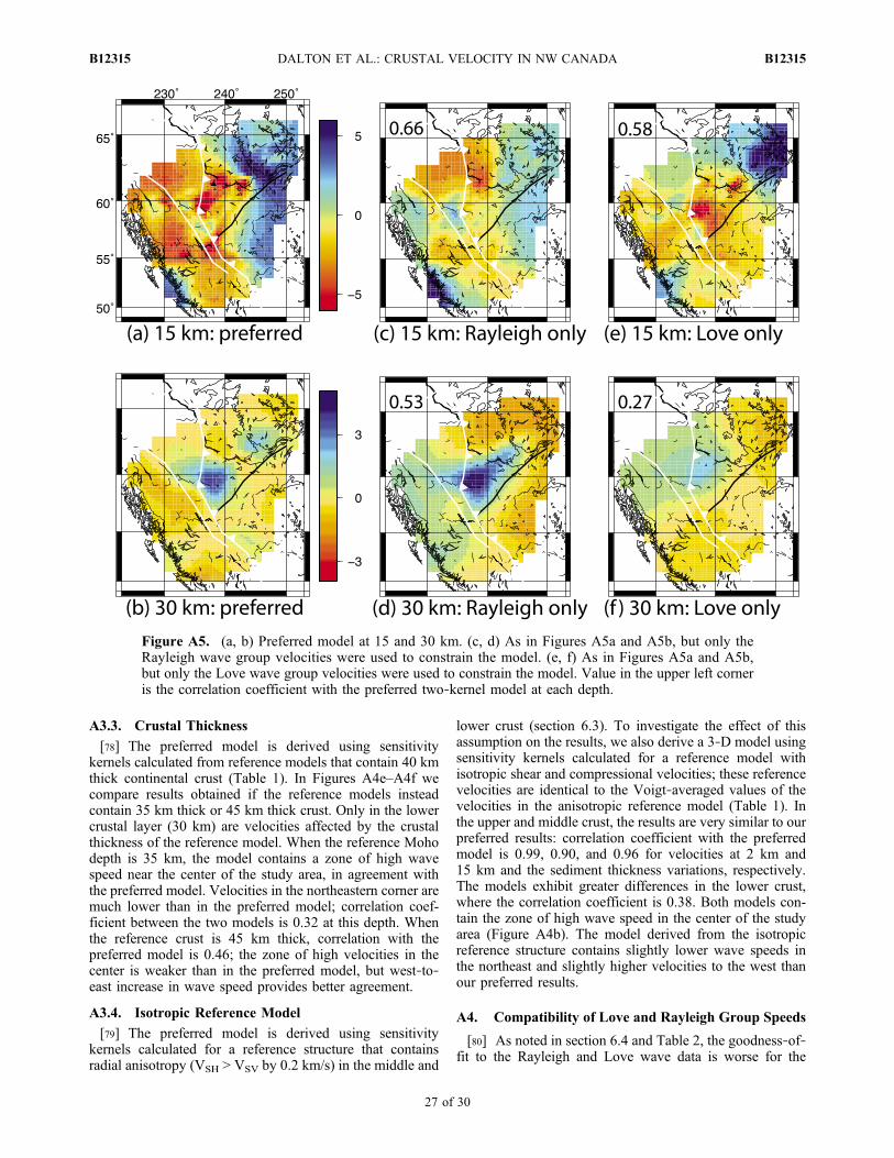
A3.3. Crustal Thickness

[78] The preferred model is derived using sensitivitykernels calculated from reference models that contain 40 kmthick continental crust (Table 1). In Figures A4e–A4f wecompare results obtained if the reference models insteadcontain 35 km thick or 45 km thick crust. Only in the lowercrustal layer (30 km) are velocities affected by the crustalthickness of the reference model. When the reference Mohodepth is 35 km, the model contains a zone of high wavespeed near the center of the study area, in agreement withthe preferred model. Velocities in the northeastern corner aremuch lower than in the preferred model; correlation coef-ficient between the two models is 0.32 at this depth. Whenthe reference crust is 45 km thick, correlation with thepreferred model is 0.46; the zone of high velocities in thecenter is weaker than in the preferred model, but west‐to‐east increase in wave speed provides better agreement.

A3.4. Isotropic Reference Model

[79] The preferred model is derived using sensitivitykernels calculated for a reference structure that containsradial anisotropy (VSH > VSV by 0.2 km/s) in the middle and

lower crust (section 6.3). To investigate the effect of thisassumption on the results, we also derive a 3‐D model usingsensitivity kernels calculated for a reference model withisotropic shear and compressional velocities; these referencevelocities are identical to the Voigt‐averaged values of thevelocities in the anisotropic reference model (Table 1). Inthe upper and middle crust, the results are very similar to ourpreferred results: correlation coefficient with the preferredmodel is 0.99, 0.90, and 0.96 for velocities at 2 km and15 km and the sediment thickness variations, respectively.The models exhibit greater differences in the lower crust,where the correlation coefficient is 0.38. Both models con-tain the zone of high wave speed in the center of the studyarea (Figure A4b). The model derived from the isotropicreference structure contains slightly lower wave speeds inthe northeast and slightly higher velocities to the west thanour preferred results.

A4. Compatibility of Love and Rayleigh Group Speeds

[80] As noted in section 6.4 and Table 2, the goodness‐of‐fit to the Rayleigh and Love wave data is worse for the

Figure A5. (a, b) Preferred model at 15 and 30 km. (c, d) As in Figures A5a and A5b, but only theRayleigh wave group velocities were used to constrain the model. (e, f) As in Figures A5a and A5b,but only the Love wave group velocities were used to constrain the model. Value in the upper left corneris the correlation coefficient with the preferred two‐kernel model at each depth.


27 of 30

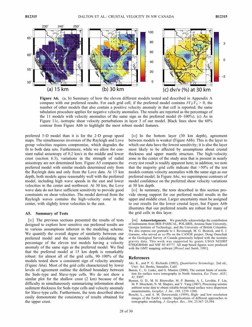
preferred 3‐D model than it is for the 2‐D group speedmaps. The simultaneous inversion of the Rayleigh and Lovegroup velocities requires compromise, which degrades thefit to both data sets. Furthermore, while we allow for con-stant radial anisotropy of 0.2 km/s in the middle and lowercrust (section 6.3), variations in the strength of radialanisotropy are not determined here. Figure A5 compares thepreferred model with similar models determined only fromthe Rayleigh data and only from the Love data. At 15 kmdepth, both models agree reasonably well with the preferredmodel, including high wave speeds in the east and lowervelocities in the center and northwest. At 30 km, the Lovewave data do not have sufficient sensitivity to provide goodconstraints on shear velocities. The model derived from theRayleigh waves contains the high‐velocity zone in thecenter, with slightly lower velocities to the east.

A5. Summary of Tests

[81] The previous sections presented the results of testsdesigned to explore how sensitive our preferred results areto various assumptions inherent in the modeling scheme.We quantify the overall degree of similarity between ourpreferred model and the test models by calculating thepercentage of the eleven test models having a velocityanomaly of the same sign as the preferred model. We findthat the preferred model at 15 km depth is remarkablyrobust: for almost all of the grid cells, 90–100% of themodels tested show a consistent sign of velocity anomaly(Figure A6a). Most of the grid cells characterized by lowerlevels of agreement outline the defined boundary betweenthe Seds‐type and Slave‐type cells. We do not show asimilar plot for the shallow crust (2 km) because of thedifficulty in simultaneously summarizing information aboutsediment thickness for Seds‐type cells and velocity anomalyfor Slave‐type cells. Furthermore, the tests described aboveeasily demonstrate the consistency of results obtained forthe upper crust.

[82] In the bottom layer (30 km depth), agreementbetween models is weaker (Figure A6b). This is the layer towhich our data have the lowest sensitivity; it is also the layermost likely to be affected by assumptions about crustalthickness and upper mantle structure. The high‐velocityzone in the center of the study area that is present in nearlyevery test result is readily apparent here; in addition, we notethat the majority grid cells indicate that >50% of the testmodels contain velocity anomalies with the same sign as ourpreferred model. In Figure A6c, we superimpose contours ofmodel confidence on the preferred shear velocity variationsat 30 km depth.[83] In summary, the tests described in this section pro-

vide strong support for our preferred model results in theupper and middle crust. Larger uncertainty must be assignedto our results for the lower crustal layer, but Figure A6billustrates that our preferred results are robust for many ofthe grid cells in this layer.

[84] Acknowledgments. We gratefully acknowledge the contributionof instruments from IRIS‐PASSCAL, POLARIS, Arizona State University,Georgia Institute of Technology, and the University of British Columbia.We also express our gratitude to J. Revenaugh, M. G. Bostock, and E. J.Garnero, who served as co‐PIs on the CANOE project. Doug Oneschukat the Geological Survey of Canada generously helped with the isostaticgravity data. This work was supported by grants USGS NEHRP07HQGR0046 and NSF 05‐45777. All map‐based figures were producedwith the GMT mapping software [Wessel and Smith, 1991].

ReferencesAki, K., and P. G. Richards (2002), Quantitative Seismology, 2nd ed.,Univ. Sci. Books, Sausalito, Calif.

Bassin, C., G. Laske, and G. Masters (2000), The current limits of resolu-tion for surface wave tomography in North America, Eos Trans. AGU,81, F897.

Bensen, G. D., M. H. Ritzwoller, M. P. Barmin, A. L. Levshin, F. Lin,M. P. Moschetti, N. M. Shapiro, and Y. Yang (2007), Processing seismicambient noise data to obtain reliable broad‐band surface wave dispersionmeasurements, Geophys. J. Int., 169, 1239–1260.

Boschi, L., and A. M. Dziewonski (1999), High‐ and low‐resolutionimages of the Earth’s mantle: Implications of different approaches totomographic modeling, J. Geophys. Res., 104, 25,567–25,594.

Figure A6. (a, b) Summary of how the eleven different models tested and described in Appendix Acompare with our preferred results. For each grid cell, if the preferred model contains dVS/VS > 0, thenumber of other models that also contain a positive velocity anomaly in that cell is reported; the sametabulation procedure applies for negative velocity anomalies. The results are reported as the percentage ofthe 11 models with velocity anomalies of the same sign as the preferred model (0–100%). (c) As inFigure 11c, isotropic shear velocity perturbations in layer 3 of our model. Black lines show the 60%contour from Figure A6b to highlight the most robust model features.


28 of 30

Bowring, S. A., and I. S. Williams (1999), Priscoan (4.00–4.03 Ga) orthog-neisses from northwestern Canada, Contrib. Mineral. Petrol., 134, 3–16.

Brocher, T. M. (2005), Empirical relations between elastic wavespeeds anddensity in the Earth’s crust, Bull. Seismol. Soc. Am., 95, 2081–2092.

Calvert, A. J., and N. Hayward (2009), Seismic imaging beneath the volca-nic rocks of the Nechako Basin, British Columbia, paper presented at2009 Joint Annual Convention, Can. Soc. Pet. Geol., Calgary, Alberta.

Cammarano, F., and B. Romanowicz (2007), Insights into the nature of thetransition zone from physically constrained inversion of long‐period seis-mic data, Proc. Natl. Acad. Sci. U. S. A., 104, 9139–9144, doi:10.1073/pnas.0608075104.

Cho, K. H., R. B. Herrmann, C. J. Ammon, and K. Lee (2007), Imaging theupper crust of the Korean Peninsula by surface‐wave tomography, Bull.Seismol. Soc. Am., 97, 198–207.

Christensen, N. I. (1996), Poisson’s ratio and crustal seismology, J. Geophys.Res., 101, 3139–3156.

Christensen, N. I., and W. D. Mooney (1995), Seismic velocity structureand composition of the continental crust: A global view, J. Geophys.Res., 100, 9761–9788.

Cook, F. A., and P. Erdmer (2005), An 1800 km cross section of the lith-osphere through the northwestern North American plate: Lessons from4.0 billion years of Earth’s history, Can. J. Earth Sci., 42, 1295–1311.

Cook, F. A., R. M. Clowes, D. B. Snyder, A. J. van der Velden, K. W. Hall,P. Erdmer, and C. A. Evenchick (2004), Precambrian crust beneath theMesozoic northern Canadian Cordillera discovered by Lithoprobe seismicreflection profiling, Tectonics, 23, TC2010, doi:10.1029/2002TC001412.

Cook, F. A., K. W. Hall, and C. E. Lynn (2005), The edge of northwesternNorth America at ∼1.8 Ga, Can. J. Earth Sci., 42, 983–997.

Courtier, A. M., J. B. Gaherty, and C. A. Dalton (2008), Mapping theMoho beneath northwest Canada: Crustal structure across CANOE,Eos Trans. AGU, 89(53), Fall Meet. Suppl., Abstract S23A‐1874.

Creaser, B., and G. Spence (2005), Crustal structure across the northernCordillera, Yukon Territory, from seismic wide‐angle studies: OminecaBelt to Intermontane Belt, Can. J. Earth Sci., 42, 1187–1203.

Crotwell, H. P., and T. J. Owens (2005), Automated receiver function pro-cessing, Seismol. Res. Lett., 76, 702–708.

Dziewonski, A. M., and D. L. Anderson (1981), Preliminary referenceEarth model, Phys. Earth Planet. Int., 25, 297–356.

Faul, U. H., and I. Jackson (2005), The seismological signature of temper-ature and grain size variations in the upper mantle, Earth Planet. Sci.Lett., 234, 119–134.

Fernandez‐Viejo, G., and R. M. Clowes (2003), Lithospheric structurebeneath the Archean Slave province and Proterozoic Wopmay orogen,northwestern Canada, from a Lithoprobe refraction/wide‐angle reflectionsurvey, Geophys. J. Int., 153, 1–19.

Fernandez‐Viejo, G., R. M. Clowes, and J. K. Welford (2005), Constraintson the composition of the crust and uppermost mantle in northwesternCanada: VP/VS variations along Lithoprobe’s SNorCLE transect, Can.J. Earth Sci., 42, 1205–1222.

Frederiksen, A. W., M. G. Bostock, and J. F. Cassidy (2001), S‐wavevelocity structure of the Canadian upper mantle, Phys. Earth Planet.Int., 124, 175–191.

Hammer, P. T. C., and R. M. Clowes (2004), Accreted terranes of north-western British Columbia, Canada: Lithospheric velocity structure andtectonics, J. Geophys. Res., 109, B06305, doi:10.1029/2003JB002749.

Harmon, N., D. Forsyth, and S. Webb (2007), Using ambient seismic noiseto determine short‐period phase velocities and shallow shear velocities inyoung oceanic lithosphere, Bull. Seismol. Soc. Am., 97, 2009–2023.

Hayward, N., and A. J. Calvert (2009), Eocene and Neogene volcanic rocksin the southeastern Nechako Basin, British Columbia: Interpretation ofthe Canadian Hunter seismic reflection surveys using first‐arrival tomog-raphy, Can. J. Earth Sci., 46, 707–720.

Hildebrand, R. S., P. F. Hoffman, and S. A. Bowring (1987), Tectono‐magmatic evolution of the 1.9 Ga Great Bear Magmatic zone, WopmayOrogen, NW Canada, J. Volcanol. Geotherm. Res., 32, 99–118.

Hoffman, P. F. (1987), Continental transform tectonics: Great Slave Lakeshear zone (ca. 1.9 Ga), northwest Canada, Geology, 15, 785–788.

Hoffman, P. F. (1988), United Plates of America, the birth of a craton:Early Proterozoic assembly and the growth of Laurentia, Annu. Rev.Earth Planet. Sci., 16, 543–603.

Jordan, T. H. (1978), Composition and development of the continentaltectosphere, Nature, 274, 544–548.

Kustowski, B., G. Ekström, and A. M. Dziewonski (2008), Anisotropicshear‐wave velocity structure of the Earth’s mantle: A global model,J. Geophys. Res., 113, B06306, doi:10.1029/2007JB005169.

Langston, C. A. (1979), Structure under Mount Rainier, Washington,inferred from teleseismic body waves, J. Geophys. Res., 84, 4749–4762.

Laske, G., and G. Masters (1997), A global digital map of sedimentthickness, Eos Trans. AGU, 78, F483.

Lee, C‐T. A. (2003), Compositional variation of density and seismic veloc-ities in natural peridotites at STP conditions: Implications for seismicimaging of compositional heterogeneities in the upper mantle, J. Geophys.Res., 108(B9), 2441, doi:10.1029/2003JB002413.

Lin, F.‐C., M. P. Moschetti, and M. H. Ritzoller (2008), Surface wavetomography of the western United States from ambient seismic noise:Rayleigh and Love wave phase velocity maps, Geophys. J. Int., 173,281–298, doi:10.1111/j.1365-246X.2008.03720.x.

Mercier, J.‐P., M. G. Bostock, J. B. Gaherty, E. J. Garnero, and J. Revenaugh(2008), The teleseismic signature of fossil subduction: NorthwesternCanada, J. Geophys. Res., 113, B04308, doi:10.1029/2007JB005127.

Mercier, J.‐P., M. G. Bostock, J. F. Cassidy, K. Dueker, J. B. Gaherty,E. J. Garnero, J. Revenaugh, and G. Zandt (2009), Body‐wave tomogra-phy of western Canada, Tectonophysics, 475, 480–492.

Mossop, G. D., and I. Shetsen (1994), Geological atlas of the WesternCanada Sedimentary Basin, Spec. Rep. 4, Alberta Geol. Surv., Edmon-ton, Alberta, Canada.

Nettles, M., and A. M. Dziewonski (2008), Radially anisotropic shearvelocity structure of the upper mantle globally and beneath NorthAmerica, J. Geophys. Res., 113, B02303, doi:10.1029/2006JB004819.

Ricketts, B. D., C. A. Evenchick, R. G. Anderson, and D. C. Murphy(1992), Bowser basin, northern British Columbia: Constraints on thetiming of initial subsidence and Stikinia‐North America terrane interac-tions, Geology, 20, 1119–1122.

Ritzwoller, M. H., N. M. Shapiro, and S‐J. Zhong (2004), Cooling historyof the Pacific lithosphere, Earth Planet. Sci. Lett., 226, 69–84.

Rodi, W. L., P. Glover, T. M. C. Li, and S. S. Alexander (1975), A fast,accurate method for computing group velocity partial derivatives forRayleigh and Love modes, Bull. Seismol. Soc. Am., 65, 1105–1114.

Rudnick, R. L., and D. M. Fountain (1995), Nature and composition ofthe continental crust: A lower crustal perspective, Rev. Geophys., 33,267–309.

Shapiro, N. M., and M. H. Ritzwoller (2004), Thermodynamic constraintson seismic inversions, Geophys. J. Int., 157, 1175–1188, doi:10.1111/j.1365-246X.2004.02254.x.

Shapiro, N. M., M. Campillo, L. Stehly, and M. H. Ritzwoller (2005),High‐resolution surface‐wave tomography from ambient seismic noise,Science, 307, 1615–1618.

Snyder, D. B., and B. J. Roberts (2007), Seismic tomographic cross‐sections of the Bowser Basin in northwest British Columbia, Canada,Bull. Can. Petrol. Geol., 55, 275–284.

Snyder, D. B., R. M. Clowes, F. A. Cook, P. Erdmer, C. A. Evenchick,A. J. van der Velden, and K. W. Hall (2002), Proterozoic prism arrestssuspect terranes: Insights into the ancient cordilleran margin from seismicreflection data, GSA Today, 12, 4–10.

Snyder, D. B., M. Pilkington, R. M. Clowes, and F. A. Cook (2009), Theunderestimated Proterozoic component of the Canadian Cordillera accre-tionary margin, in Earth Accretionary Systems in Space and Time, Geol.Soc. Spec. Publ., 318, 257–271.

Takeuchi, H., and M. Saito (1972), Seismic surface waves, in Methods inComputational Physics, vol. 11, edited by B. A. Bolt, pp. 217–295,Academic, New York.

Tsai, V. C. (2009), On establishing the accuracy of noise tomographytravel‐time measurements in a realistic medium, Geophys. J. Int., 178,1555–1564.

Van der Lee, S., and A. Frederiksen (2005), Surface wave tomographyapplied to the North American upper mantle, in Seismic Earth: ArrayAnalysis of Broadband Seismograms, Geophys. Monogr. Ser., vol. 157,edited by A. Levander and G. Nolet, pp. 67–80, AGU, Washington, D. C.

Webb, S. C. (1998), Broadband seismology and noise under the ocean, Rev.Geophys., 36, 105–142.

Welford, J. K., R. M. Clowes, R. M. Ellis, G. D. Spence, I. Asudeh, andZ. Hajnal (2001), Lithospheric structure across the craton‐Cordillerantransition of northeastern British Columbia, Can. J. Earth Sci., 38,1169–1189.

Wessel, P., and W. H. F. Smith (1991), Free software helps map and displaydata, Eos Trans. AGU, 72(41), 441.

Yang, Y., M. H. Ritzwoller, A. L. Levshin, and N. M. Shapiro (2007),Ambient noise Rayleigh wave tomography across Europe, Geophys.J. Int., 168, 259–274.

Yao, H., X. Campman, M. V. de Hoop, and R. D. van der Hilst (2009),Estimation of surface wave Green’s functions from correlations of directwaves, coda waves, and ambient noise in SE Tibet, Phys. Earth Planet.Inter., 177, 1–11, doi:10.1016/j.pepi.2009.07.002.

Zelt, C. A., R. M. Ellis, and B. C. Zelt (2006), 3‐D structure across theTintina strike‐slip fault, northern Canadian Cordillera, from seismicrefraction and reflection tomography, Geophys. J. Int., 167, 1292–1308.


29 of 30

Zhu, L., and H. Kanamori (2000), Moho depth variation in SouthernCalifornia from teleseismic receiver functions, J. Geophys. Res., 105,2969–2980.

A. M. Courtier, Department of Geology and Environmental Science,James Madison University, Harrisonburg, VA 22807, USA.

C. A. Dalton, Department of Earth Sciences, Boston University, Boston,MA 02215, USA. ([email protected])J. B. Gaherty, Lamont‐Doherty Earth Observatory, Earth Institute at

Columbia University, Palisades, NY 10964, USA.


30 of 30

Documents

Crustal VS structure in northwestern Canada: Imaging … · Crustal VS structure in northwestern Canada: Imaging the Cordillera‐craton transition with ambient noise tomography