CRUISE REPORTEco-FOCI’s Bering Sea Ice Edge ‘06

Cruise Number: TN193FOCI Number:01TT06

Ship: R/V Thomas G. Thompson

Area of Operations: Bering Sea Ice EdgeDeparture: Kodiak – April 12, 2006Personnel Exchange: St. Paul Is., April 29, 2006Arrival: Seward, AK – May 13, 2006

Participating Organizations and Principal Investigators:

Dr. Phyllis StabenoNOAA – Pacific Marine Environmental Laboratory (PMEL)7600 Sand Point Way N.E.Seattle, Washington 98115-6439

Dr. Jeff NappNOAA – Alaska Fisheries Science Center (AFSC)7600 Sand Point Way N.E.Seattle, Washington 98115-0070

Dr. George Hunt/ David HyrenbachSchool of Fisheries and Aquatic ScienceBox 355020University of WashingtonSeattle, Washington 98195

Dr. Lisa EisnerAuke Bay LaboratoryNOAA – Alaska Fisheries Science Center (AFSC) 11305 Glacier Hwy.Juneau, AK 99801

Dr. Melissa ChiericiDepartment of Chemistry/ Marine ChemistryGöteborg University412 96 Göteborg, Sweden

Chief Scientist:Dr. Nancy Kachel, NOAA/PMEL206-526-6780Nancy Kachel@noaa.gov

Personnel: Leg 1Dr. Phyllis J. Stabeno USA PMELDr. Calvin Mordy USA PMELDr. George Hunt, Jr. USA UWDr. Edward Cokelet USA PMELDr. David Hyrenbach Spain UW/DukeDr. Lisa Eisner USA AFSC/Auke Bay LabDavid G. Kachel USA PMELMargaret Sullivan USA PMELRachael Cartwright USA AFSCColleen Harpold USA AFSCCarolina Parada Chile AFSCKathy Mier USA AFSCElizabeth Logerwell USA AFSCMichael Cameron USA NMMLShawn Dahle USA NMMLRobert Montgomery USA NMMLElizabeth Jenkinson USA NMMLCharlie Saccheus USA AK NativeJohn Goodwin Sr. USA AK NativeEvgeniy Mamev Russia NMML

Personnel: Leg 2Dr. Jeffrey Napp USA AFSCDr. Calvin Mordy USA PMELDr. George Hunt, Jr. USA UWDr. David Hyrenbach Spain UW/DukeDr. Carol Ladd USA PMELDr. Edward Cokelet USA PMELDr. John Bengtson USA NMMLDr. Lisa Eisner USA AFSC/Auke Bay LabDavid G. Kachel USA PMELMargaret Sullivan USA PMELRachael Cartwright USA AFSCMorgan Busby USA AFSCColleen Harpold USA AFSCMatt Wilson USA AFSCMichael Cameron USA NMMLShawn Dahle USA NMMLRobert Montgomery USA NMMLElizabeth Jenkinson USA NMMLCharlie Saccheus USA AK NativeJohn Goodwin Sr. USA AK Native

Sandi Doughton USA The Seattle TimesSteven Ringman USA The Seattle TimesSoames Summerhays UK Summerhays Films

Objectives of Cruise:This cruise was a collaboration among the NOAA’s Fisheries and Oceanography

Coordinated Investigations (FOCI), which is a joint program between the Pacific Marine Environmental Laboratory (PMEL) and the Alaska Fisheries Science Center (AFSC), the National Marine Mammal Laboratory (NMML); and the Marine Assessment & Conservation Engineering Program (MACE). Support was provided by NOAA, the North Pacific Research Board (NPRB) and the Alaska Ocean Obserivng System (AOOS). NOAA researchers were joined by scientists from the University of University of Washington, Duke University, and the University of Göteborg, Sweden. (The latter was involved in post-cruise analysis of samples collected for her). In addition, two experienced Native Americans came to assist the scientists from the NMML in seal tagging observations. A Russian photographer also accompanied the NMML operations during the first leg. During Leg 2, a reporter and photographer,Sandi Doughton and Steven Ringman from The Seattle Times, and a filmmaker, Soames Summerhays came aboard to document our research efforts.

The primary purpose of this cruise is: to observe the ice-edge ecosystem of the eastern Bering Sea, and especially, to investigate the role of the ice edge may have in that ecosystem. Our sampling targeted the distribution of physical, biological, and chemical properties (T, S, nutrients, chlorophyll) of the water column across the zone of the ice-edge, and within the ice floes, with special attention to the epontic algae and metazoan communities. We sampled water column algae and zooplankton communities that are utilizing the phytoplankton bloom associated with the presence of the ice, and observing the distribution of birds and mammals that utilize the ice floes in the spring. Ribbon seals, in particular, were the focus of the marine mammal component. Tagging of ribbon seals with ARGOS transmitters permits NMFS/ NMML personnel to track the movements of these little-known animals after the ice melts. Finally, during the two-ship operations, personnel on Miller Freeman used hydro-acoustics to search for concentrations of fish at and behind the ice edge. Divers from Miller Freeman sampled and photographed planktonic organisms attached or congregating underneath individual ice floes.

The conductivity, temperature and depth (CTD) casts were made with a SeaBird 911 with dual temperature and conductivity sensors. Attached to the CTD were sensors measuring oxygen, transmission (beam attenuation), fluorescence, and fluorescence spectra (with an AC-9 instrument). Water sampling was done for chlorophyll, nutrients, salinity, epi-fluorescence, alkalinity, dissolved inorganic carbon (on one line) and phytoplankton species identification slides. We also collected samples for phytoplankton productivity incubations. Zooplankton sampling was done using the following types of gear: MARMAP bongo tows with 60 and 20 cm bongos, with .333 and 0.128mm mesh nets; CalVET tows; vertical ring-net tows; and Tucker trawls for crab larvae. Copepods were collected for egg production experiments.

On three occasions, trips were made to sample ice floes. At each station, ice cores were taken to sample chlorophyll and phytoplankton, and meson-plankton species in the ice, salinity, nutrients, and alkalinity. Holes were drilled to sample pore water properties, and surface waters were taken. This scheme allows us to compare the properties within the ice floe and pore water and those in the immediately adjacent surface water.

Bird and mammal observations were made along the ice edge, and bird observations were also taken on lines perpendicular and parallel (but at distance) away from the ice edge. The scientists from the NMML tagged both adult and pup seals via small boat operations. On-deck incubation experiment to measure phytoplankton growth and shipboard incubations to estimate zooplankton egg production rates were made.

Cruise Summary:The R/V Thomas G. Thompson departed Kodiak, AK to begin Eco-FOCI’s “Bering

Sea Ice ’06” cruise at 1455ADT on April 12, 2006 with a storm approaching the area. We were fortunate to have in command Captain Phil Smith, who has had many years’ experience piloting ships in the coastal waters of Alaska and in the Bering Sea. He chose to take the ship through Whale Pass, into Shelikof Strait for the transit to Unimak Pass and the Bering Sea.

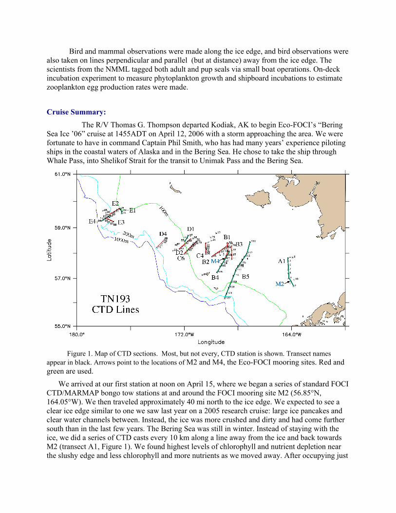
Figure 1. Map of CTD sections. Most, but not every, CTD station is shown. Transect names appear in black. Arrows point to the locations of M2 and M4, the Eco-FOCI mooring sites. Red and green are used.

We arrived at our first station at noon on April 15, where we began a series of standard FOCI CTD/MARMAP bongo tow stations at and around the FOCI mooring site M2 (56.85°N, 164.05°W). We then traveled approximately 40 mi north to the ice edge. We expected to see a clear ice edge similar to one we saw last year on a 2005 research cruise: large ice pancakes and clear water channels between. Instead, the ice was more crushed and dirty and had come further south than in the last few years. The Bering Sea was still in winter. Instead of staying with the ice, we did a series of CTD casts every 10 km along a line away from the ice and back towards M2 (transect A1, Figure 1). We found highest levels of chlorophyll and nutrient depletion near the slushy edge and less chlorophyll and more nutrients as we moved away. After occupying just

one CTD transect, another storm arrived, so we transited to the area around FOCI mooring M4 (57.83°ZN, 168.82°W). We again occupied a set of standard FOCI stations around M4. See Figure 1 for location of the mooring and CTD sites.

to distinguish different transects from one another.

North of M4 at CTD017 the ice edge was solid, and air temperatures were –10 to –12°C. We experience difficulties with both our CTD, the SeaCat attached to the bongo, and our Niskin bottles freezing on deck. All equipment needed to be brought in to the protected staging bay between deployments from then until the last day of sampling. Our sampling plan was to move northwestwardly along the ice edge during daylight hours, and then to make CTD/bongo transects out of the ice during the night. During the day, productivity experiments, and bird and mammal observations were interrupted for periodic CTD Bongo stations. The shape of the ice edge at this time was highly irregular, resembling a coastline with fjords and peninsulas. Generally stormy conditions prevented us from conducting excursions onto the ice for coring operations until later in the cruise. Operations continued in this manner through April 22 (Transect lines with Ids starting with B and C).

On April 23, we began joint operation with the NOAAShip Miller Freeman. We went one bird observer over to the Freeman for this time. The Freeman conducted hydro-acoustic surveys in the area in search of fish, but found insufficient signals to warrant trawling operations. They also executed two dive operations under ice floes to collect algal samples from under the ice, and to take photographs there.

By April 24, another storm that set in, with winds blowing between 35 and 40 knots all day. Air temperature was between -9º C and -8º C. The first attempt to tag seals proved unsuccessful.

Late that night, it snowed hard, which limited visibility severely. When we headed back to the ice edge the next morning we found ice broken up into very small ice-cube sized pieces mixed with larger, broken pieces, all lined up along wind lines. Bird observations were halted mid-day due to limited visibility and storm conditions.

After two days locked down due to the storm, on the evening of April 26 we resumed operations. (Transect IDs beginning with D).

On April 27.the first successful tagging of seals took place.

On April 28, we again exchanged personnel with the Freeman, which then departed our area of operations. The Thompson steamed south to the Pribilof Islands. We occupied one station just west of St. Paul Island, a site visited on the July-August 2004 Pribilof cruise, to contrast the chemistry and biology at this time of year near the islands with that found during the summer, and with our findings near the ice. We used small boat operations in the harbor at St. Paul to debark/embark some members of the science party for the second leg of the cruise.

We began the second leg by returning north, we encountered heavy bands of ice in the area we had sampled only 24 hours previously. The long period of northerly winds had broken up the ice and formed it into long strips of 80-100 percent ice, that were moving south to southwestwardly at a rate of approximately 20 miles per day. This movement can be seen on the map in Figure 2, which shows the sea-chest temperatures along the cruise track, as well as the National Ice center’s prediction of the location of the marginal ice zone edge on various dates during the cruise.

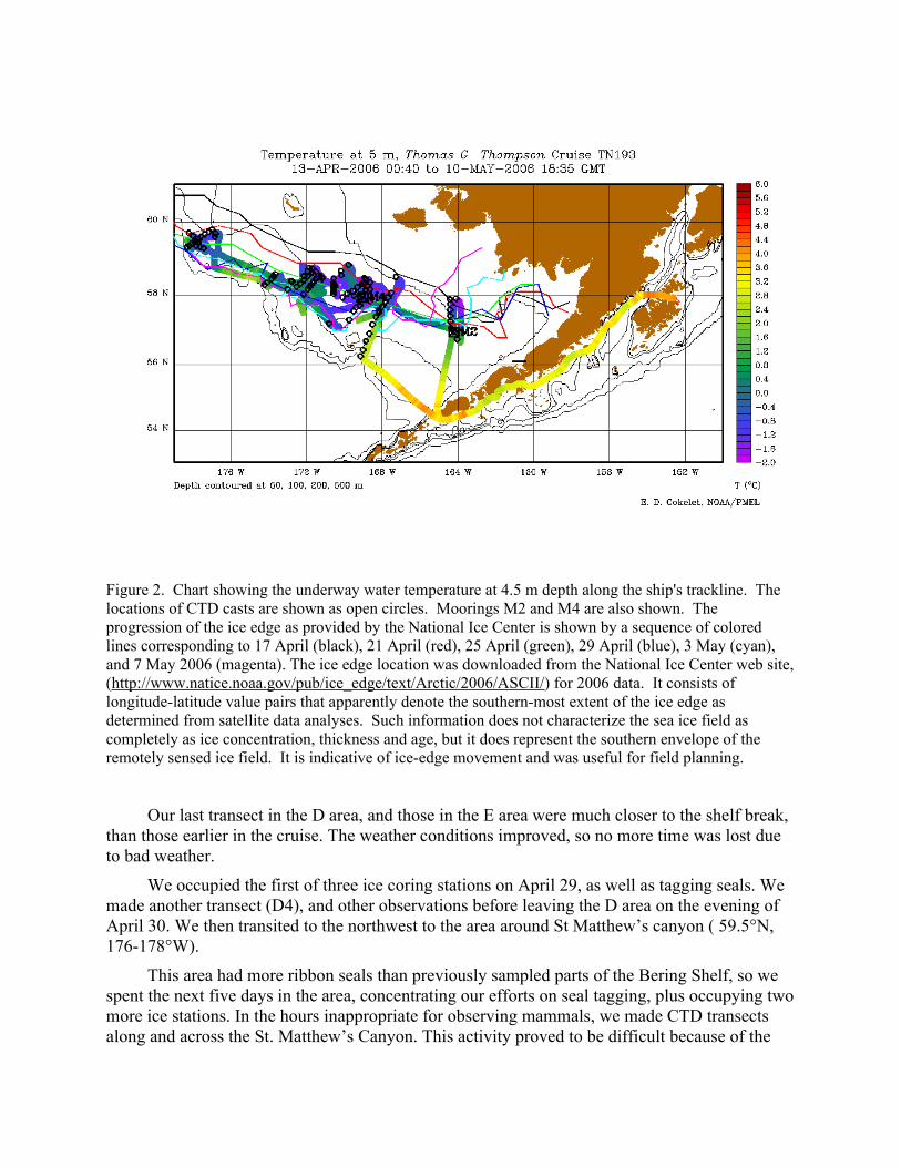
Figure 2. Chart showing the underway water temperature at 4.5 m depth along the ship's trackline. The locations of CTD casts are shown as open circles. Moorings M2 and M4 are also shown. The progression of the ice edge as provided by the National Ice Center is shown by a sequence of colored lines corresponding to 17 April (black), 21 April (red), 25 April (green), 29 April (blue), 3 May (cyan), and 7 May 2006 (magenta). The ice edge location was downloaded from the National Ice Center web site, (http://www.natice.noaa.gov/pub/ice_edge/text/Arctic/2006/ASCII/) for 2006 data. It consists of longitude-latitude value pairs that apparently denote the southern-most extent of the ice edge as determined from satellite data analyses. Such information does not characterize the sea ice field as completely as ice concentration, thickness and age, but it does represent the southern envelope of the remotely sensed ice field. It is indicative of ice-edge movement and was useful for field planning.

Our last transect in the D area, and those in the E area were much closer to the shelf break, than those earlier in the cruise. The weather conditions improved, so no more time was lost due to bad weather.

We occupied the first of three ice coring stations on April 29, as well as tagging seals. We made another transect (D4), and other observations before leaving the D area on the evening of April 30. We then transited to the northwest to the area around St Matthew’s canyon ( 59.5°N, 176-178°W).

This area had more ribbon seals than previously sampled parts of the Bering Shelf, so we spent the next five days in the area, concentrating our efforts on seal tagging, plus occupying two more ice stations. In the hours inappropriate for observing mammals, we made CTD transects along and across the St. Matthew’s Canyon. This activity proved to be difficult because of the

nearly ubiquitous strips of ice encountered in almost any direction. The strips of ice in this area were heavier than previously encountered, and contained thicker chucks and stacks of ice. This ice, most probably had bed piled up behind St. Matthew’s island, and was now being transported around to the south and then west. Some of it appeared to have been fast ice at one time. We began to observe higher fluorescence near the surface, but not a full spring bloom while we were in this area.

On the evening of May 5, we left the westernmost area in order to return to the area around M$, which we had previously sampled two weeks earlier. En route, we used Tucker trawls to take stratified samples of zooplankton, in a location where crab (zoea) had been found, at the southwest end of the D2 line.

We then proceeded to travel back to M4. In our absence the marginal ice edge, with its vast network of ice strips had moved south, nearly to St. Paul Is. (Fig 2). The ship needed to pick its way through and around many such strips in order to work its way south and east of M4. The first line (B4) running northeast-southwest through this site encountered heavy ice at all but the last station. The National Ice Center web site predicted that forty miles to the east there was an open area, so we chose to sample a long transect from near the inner shelf to the edge of Pribilof canyon through that area (line B5).

We ended operations at 1500ADT on May 9, 2006. We then transited back to Seward, AK, arriving at 1430 on May 12, 2006.

Sampling MethodsA. Water Property Measurements and Sampling - Nancy Kachel, Calvin Mordy, Ned Cokelet, David Kachel, Peggy Sullivan, Phyllis Stabeno, and Carol LaddCTD Casts and Sampling

A total of 122 CTD casts were made. Of those, 108 casts collected water samples.

The SeaBird 911 plus CTD was equipped with dual temperature and conductivity sensors, plus a fluorometer, SBE042 Oxygen sensor, Photosythetically Activated Radiation was made using a 2-Pi sensor (not 4 PI, as is typical for Eco- FOCI operations) and a transmissometer were attached. Lisa Eisner of Auke Bay Laboratories also attached an AC-9 spectral fluorescence sensor to the CTD cage. It collected data internally, not as part of the SeaBird 911 data stream (see below). Chlorophyll samples (786) were filtered onto GFF filters and frozen and stored for later analysis at AFSC. Salinity samples were taken for the purpose of calibrating the CTD salinity results.

Water samples for dissolved inorganic nutrients (NO3–, NO2

–, HPO42–, and H2SiO4

2–) were collected using 5-liter Niskin bottles. Nutrient samples were filtered during sampling to remove particulates. The samples were analyzed onboard within 8 hours after collection. Phosphate concentrations were determined using a Technicon AutoAnalyzer II; silicic acid, nitrate and nitrite concentrations were determined using components from Alpkem and Perstorp instrumentation. Analytical methods were from Armstrong et al. (1967) and Atlas et al. (1971). Standardization and analysis procedures specified by Gordon et al. (1993) were closely followed including calibration of labware, preparation of primary and secondary standards, and

corrections for blanks and refractive index. Nitrate and phosphate were accurate to <2% full scale (<1 µM nitrate and <0.06 µM phosphate.

Alkalinity samples were collected on several CTD lines for analysis by Melissa Chierci, at the University of Gotborg, Sweden. On Line B5, DIC (dissolved inorganic carbon) samples were also collected for her. At those stations, POC (particulate organic carbon) samples were taken for Jeff Napp.

A summary of the gear used and the samples collected is contained in the Appendix Tables 1 and 2.

Flow-Through SamplingThe NAS-3X nitrate meter was installed as part of the underway instrument suite and on

moorings in the GOA. This instrument uses standard wet chemistry techniques for measuring nitrate. The sample is passed through a column filled with copperized Cd-Ag wire where nitrate is reduced to nitrite. The nitrite is formed into a red azo dye by complexing with sulfanilamide and N-1-naphthylethylenediamine, and the absorbance of the complexed nitrite is measured spectrophotometrically. The underway nitrate meters were configured to sample about every 30 minutes and standards were analyzed every 4th sample (2003) or with every sample (2004). For the moored nitrate meters, seawater samples and calibration standards were analyzed at 6-hr intervals. In both modes, blanks were analyzed prior to each measurement, and consisted of measuring the absorbance of a standard or sample without reagents. Working standards were made in low-nutrient seawater (LNSW) with a known nitrate. Because the NAS-3X does not include separate measurements for nitrate and nitrite, results from these instruments are reported as nitrate+nitrite, (N+N).

Discrete nutrient samples were drawn approximately every 6 hours for both chlorophyll and nutrient analyses. These samples were treated in the same manner as the other samples.

B. Ice Core Operations- Peggy Sullivan, Ned Cokelet, Calvin Mordy, Nancy Kachel and Lisa Eisner

Due to limiting weather and sea conditions during the first leg of the cruise, no ice floe operations were conducted. During leg two, three ice floe operations were completed. For ice floe samples, the following were recorded: GPS position, ice thickness, freeboard, snow depth, estimated floe size, and floe description. Table 1 summarizes the ice samples taken.

On each ice floe operation three cores were collected using an Austin Kovaks 9 cm diameter ice corer. The cores were designated as 1) chlorophyll (color-coded green), 2) salinity/nutrients/alkalinity (color-coded red), and 3) temperature and productivity (color-coded yellow). All cores were placed on core cutting surface, measured from the top of core and photographed, with banding and features noted. Cores #1 and #2 were sawed into 10 cm sections starting at the bottom, with top section usually greater than 10 cm. Core #3 had small holes drilled 10 cm apart on the 5-cm mark for measuring ice temperature over the length of the column. The bottom 5 cm was saved as a production sample. Other parts of temperature core were saved from two of the three cores. All samples were placed into color-coded, station-labeled Ziploc bags and put into a cooler. After the first core, a black tarp cover was devised so core would be protected from excess light during sectioning.

At core hole #1, a 4-π PAR sensor was inserted into the hole and under ice. A 2π PAR sensor was used above ice surface. Three time-separated PAR readings were recorded as pairs (above and below ice) along with UTC time. One set of PAR readings was taken from core hole #3 for use with production sample.

After the first core on each sampled ice floe, brine holes were drilled at varying depths with a 6 inch ice auger to allow hole to re-fill with sea water for collecting samples integrated to the particular depth. Target depths were 20, 40, 60 and 80 cm. Not all floes were thick enough to warrant brine hole samples. Holes had slush removed before being left to fill. Near the end of operations, a bilge pump suctioned brine samples into 1-gallon Ziploc bags. Samples were placed in a cooler. Just before leaving the ice floe a one-liter surface water sample and a final GPS reading were taken.

Upon return to the ship, samples were double bagged. Core #1: each section was mixed with 1 liter of filtered sea water. Thawed sample (1-3 days thaw) was mixed well, volume measured and split up into 5 separate samples for chlorophyll, phytoplankton, lugols (micro zooplankton), phytoplankton species and POC. Core #2: Thawed sample volume was measured and split into 3 separate samples for bottle salinity, nutrients, and alkalinity. Core #3: The bottom 5 cm of the core was diluted with filtered seawater and used for primary production experiments (See next section). This core was also used for comparison chlorophyll, species, and nutrients.

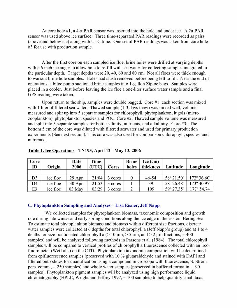
Table 1. Ice Operations - TN193, April 12 - May 13, 2006

Core ID Origin

Date 2006

Time (UTC) Cores

Brine holes

Ice (cm) thickness Latitude Longitude

D3 ice floe 29 Apr 21:04 3 cores 0 46-54 58º 21.50' 172º 36.60'D4 ice floe 30 Apr 21:53 3 cores 1 39 58º 26.48' 173º 40.97'E3 ice floe 03 May 03:29 3 cores 2 109 59º 27.35' 177º 54.74

C. Phytoplankton Sampling and Analyses – Lisa Eisner, Jeff NappWe collected samples for phytoplankton biomass, taxonomic composition and growth

rate during late winter and early spring conditions along the ice edge in the eastern Bering Sea. To estimate total phytoplankton biomass and biomass within different size fractions, discrete water samples were collected at 6 depths for total chlorophyll a (Jeff Napp’s group) and at 1 to 4 depths for size fractionated chlorophyll a (> 10 µm, > 5 µm, and > 2 µm fractions, ~ 400 samples) and will be analyzed following methods in Parsons et al. (1984). The total chlorophyll samples will be compared to vertical profiles of chlorophyll a fluorescence collected with an Eco fluorometer (WetLabs) on the CTD. Phytoplankton taxonomic composition will be determined from epifluorescence samples (preserved with 10 % glutaraldehyde and stained with DAPI and filtered onto slides for quantification using a compound microscope with fluorescence, S. Strom pers. comm., ~ 250 samples) and whole water samples (preserved in buffered formalin, ~ 90 samples). Phytoplankton pigment samples will be analyzed using high performance liquid chromatography (HPLC, Wright and Jeffrey 1997, ~ 100 samples) to help quantify small taxa,

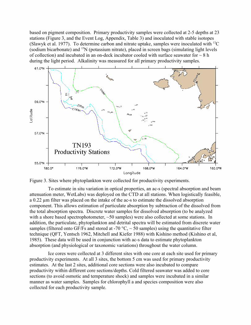
based on pigment composition. Primary productivity samples were collected at 2-5 depths at 23 stations (Figure 3, and the Event Log, Appendix, Table 3) and inoculated with stable isotopes (Slawyk et al. 1977). To determine carbon and nitrate uptake, samples were inoculated with 13C (sodium bicarbonate) and 15N (potassium nitrate), placed in screen bags (simulating light levels of collection) and incubated in an on-deck incubator cooled with surface seawater for ~ 8 h during the light period. Alkalinity was measured for all primary productivity samples.

Figure 3. Sites where phytoplankton were collected for productivity experiments.

To estimate in situ variation in optical properties, an ac-s (spectral absorption and beam attenuation meter, WetLabs) was deployed on the CTD at all stations. When logistically feasible, a 0.22 µm filter was placed on the intake of the ac-s to estimate the dissolved absorption component. This allows estimation of particulate absorption by subtraction of the dissolved from the total absorption spectra. Discrete water samples for dissolved absorption (to be analyzed with a shore based spectrophotometer, ~50 samples) were also collected at some stations. In addition, the particulate, phytoplankton and detrital spectra will be estimated from discrete water samples (filtered onto GF/Fs and stored at -70 °C, ~ 50 samples) using the quantitative filter technique (QFT, Yentsch 1962, Mitchell and Kiefer 1988) with Kishino method (Kishino et al, 1985). These data will be used in conjunction with ac-s data to estimate phytoplankton absorption (and physiological or taxonomic variations) throughout the water column.

Ice cores were collected at 3 different sites with one core at each site used for primary productivity experiments. At all 3 sites, the bottom 5 cm was used for primary productivity estimates. At the last 2 sites, additional core sections were also incubated to compare productivity within different core sections/depths. Cold filtered seawater was added to core sections (to avoid osmotic and temperature shock) and samples were incubated in a similar manner as water samples. Samples for chlorophyll a and species composition were also collected for each productivity sample.

References for This Section:Kishino, M., M. Takahashi, N. Okami, and S. Ichimura. 1985. Estimation of the spectral absorption coefficients of phytoplankton in the sea. Bull. Mar. Sci. 37: 634-642.

Mitchell, B.G., and D.A. Kiefer. 1988. Chlorophyll a specific absorption and fluorescence excitation spectra for light-limited phytoplankton. Deep Sea Res. 35: 639-663.

Parsons, T.R., Y. Maita and C. M. Lalli. 1984. A manual of chemical and biological methods for seawater analysis. Pergamon Press.

Slawyk, G., Y. Collos and J.C. Auclair. 1977. The use of the 13C and 15N isotopes for the simultaneous measurement of carbon and nitrogen turnover rate in marine phytoplankton. Limnol. Oceanogr.

Wright, S.W., and S.W. Jeffrey. 1997. High-resolution HPLC system for chlorophylls and carotenoids of marine phytoplankton, p.327-341. In: S.W. Jeffrey, R.F. Mantoura, and S.W. Wright [eds.], Phytoplankton pigments in oceanography: guidelines to modern methods. Unesco Publishing.

Yentsch, C.S. 1962. Measurement of visible light absorption by particulate matter in the ocean. Limnol. Oceanogr. 7: 207-217.

D. Zoo- and Ichthyoplankton Sampling - Jeff Napp, Collen Harpold, Rachael Cartwright, Carolina Parada, Matt Wilson, and Morgan BusbyZoo- & Ichthyoplankton patterns:

Ninety-five tows of 20 & 60 cm bongo frames with 153 and 333 µm mesh, respectively were used to collect plankton samples along and between transect lines. A subsample of the catch from Net 2 of the 60 cm bongo frame was inspected at every station. For most of the cruise, only a small number of larvae were found and rarely were they pollock. Very late in the cruise, upon returning to the B lines (B4 & B5) many gadid eggs and larvae were observed. The majorities of eggs were much larger than walleye pollock and are thought to be the eggs of Boreogadus saida, the arctic cod. The larvae were difficult to identify, but were thought to be a mixture of pollock and arctic cod. The only other station where appreciable numbers of fish larvae were found was at Station E4H5 where rockfish larvae (Sebastes spp.) were abundant.

Subsamples from Net 2 were also examined for crab larvae. We were primarily interested in finding the larvae of snow crab (Chionoecetes opilio). Zoea Stage I crab larvae were found on several transects on the D line (D3H1, D3H2, D4H2). The larvae were first spotted just before the mid-cruise transfer of scientists, then again, just after the transfer. We accomplished an abbreviated series of tows for vertical distribution at D4H2, but had to leave the area soon thereafter before we could complete a more extensive set of tows. After we finished the E transects we returned to the area where we estimated they had been advected during the intervening time. We found them on the first tow and accomplished two series of Tucker trawls for vertical distribution. The crab zoeas were tentatively identified as snow crab larvae; a more detailed analysis will be accomplished in Seattle.

In the process of inspecting the subsample from Net #2 for fish and crab larvae, we also obtained an impression of the composition of the zooplankton. In general, the stations with high phytoplankton also had low zooplankton biomass. In addition, the boundaries between slope/ oceanic species and middle shelf species were not located where they would normally be in the spring and summer. Some of the time, there did appear to be some correspondence between stations of high biomass of outer shelf species with observations of planktivorous birds in attendance. Chaetognaths were very abundant at some stations and Calanus marshallae adult females were difficult to find. Euphausiids were fairly abundant in many of the study areas. Copepod abundances were low during the first leg of the cruise; those that were present were early copepodites of Neocalanus plumchrus/flemingeri at area B. In general, area D seemed to have the most diverse copepod community: including Neocalanus plumchrus/flemingeri, early stage N. cristatus, Metridia spp., Pseudocalanus spp. and a few Calanus marshallae.

Three CalVET samples each (53 µm) were obtained around Moorings 2 and 4. These samples, obtained early during the cruise will tell us how many copepod nauplii were in the water column during that time.

See the Appendix Tables 1 and 2 for a summary of the gear used and the samples collected.

Plankton Processes: Several different projects were attempted to measure rate processes or condition of

organisms at and near the ice edge. The first project was to analyze the RNA / DNA ratios of

pollock larvae to determine their condition. Unfortunately, due to the very cold spring and the timing of the cruise, very few pollock larvae were encountered and larvae removed from the standard bongo tows were beat up and may not be suitable for analysis.

Low temperature egg production experiments were planned for Calanus marshallae since global egg production models lack data below 5 ºC. The storminess during the early part of the cruise precluded doing experiments early on, and lack of C. marshallae during the latter part of the cruise made it difficult, also. Only one experiment was attempted. Twenty adult females were incubated for 24 hr at 0 ºC. Approximately one-half laid clutches of eggs.

Collection of fatty acid profiles for Calanus and euphausiids were also planned for the cruise. The FA profiles were to be compared with profiles obtained during the summer of 2004 around the Pribilof Islands. Unfortunately, the storminess during the early part of the cruise made it impossible to accomplish this early on. Near the end of the cruise, a sufficient number of euphausiids (Thysanoessa raschii) were captured in Net 2 of the bongo to freeze for FA analyses. We never encountered enough C. marshallae for the same samples.

Chlorophyll Sampling: Water sampling for vertical profiles of total chlorophyll was conducted at all CTD

stations. Typically 6 depths were sampled in each cast (112 casts and 671 samples). The samples were frozen and will be processed in Seattle after the cruise. Samples for total chlorophyll were also obtained from sections of the ice cores to compare with the amount in the water column. These same stations / ice cores also supplied samples for particulate organic carbon and nitrogen.

Micro-zooplankton Sampling:Water samples for micro-zooplankton were taken on some of the CTD casts and a few

of the ice cores to compare the micro-zooplankton biomass and community composition in the water column and in the ice. All samples were preserved with acid Lugol’s and will be transported to Dr. Suzanne Strom’s laboratory at the Shannon Point Marine Laboratory.

E. Seabird and Cetacean Sightings (April 13 – May 12, 2006), George L. Hunt, Jr., K. David Hyrenbach and Elizabeth Logerwell

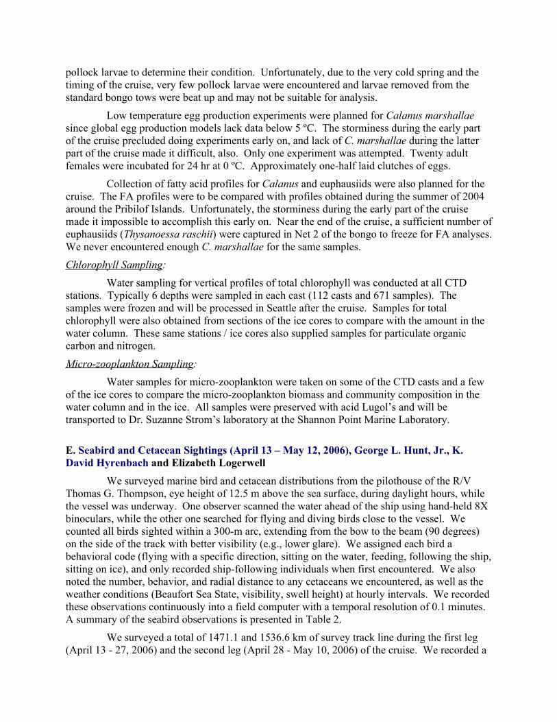
We surveyed marine bird and cetacean distributions from the pilothouse of the R/V Thomas G. Thompson, eye height of 12.5 m above the sea surface, during daylight hours, while the vessel was underway. One observer scanned the water ahead of the ship using hand-held 8X binoculars, while the other one searched for flying and diving birds close to the vessel. We counted all birds sighted within a 300-m arc, extending from the bow to the beam (90 degrees) on the side of the track with better visibility (e.g., lower glare). We assigned each bird a behavioral code (flying with a specific direction, sitting on the water, feeding, following the ship, sitting on ice), and only recorded ship-following individuals when first encountered. We also noted the number, behavior, and radial distance to any cetaceans we encountered, as well as the weather conditions (Beaufort Sea State, visibility, swell height) at hourly intervals. We recorded these observations continuously into a field computer with a temporal resolution of 0.1 minutes. A summary of the seabird observations is presented in Table 2.

We surveyed a total of 1471.1 and 1536.6 km of survey track line during the first leg (April 13 - 27, 2006) and the second leg (April 28 - May 10, 2006) of the cruise. We recorded a

total of 21,949 seabirds, and identified 19,105 (87.1%) belonging to 26 different species. Six “common” species together accounted for 97 % of all the identified birds: the Black-legged Kittiwake (28.1%), the Glaucous Gull (24.1%), the Northern Fulmar (17.5%), the Thick-billed Murre (15.6%), the Common Murre (8.0%), and the Glaucous-winged Gull (3.6%). These locally breeding species largely forage on fish, even though they also consume euphausiids and large medusae. Zooplankton-feeding seabirds were largely absent; though we encountered low numbers of Parakeet Auklets (1.1%), generalist feeders known to consume euphausiids and larval fish, and Least Auklets (0.2%), plankton specialists known to feed on copepods.

We also encountered several rare species during our survey. Most notably, we documented the occurrence of two Siberian (Vega and Slaty-Backed) and an Arctic (Ivory) gulls in the Bering Sea shelf. We also encountered endemic Red-legged Kittiwakes in the vicinity of St. George Island and Pribilof Canyon. In spite of their vast numbers in spring/summer (May - August) in the Bering Sea, with an estimated population of 9 - 20 million, we only encountered a few hundred Short-tailed Shearwaters on the south side of Unimak Pass on May 10th, while sailing back to Seward.

The remaining 2,844 (12.9%) birds were identified to genus or family. Three pairs of closely related species, which are difficult to identify at-sea, accounted for 98% of these unidentified sightings. Unidentified murres (Common or Thick-billed), unidentified gulls (Glaucous or Glaucous-winged), and dark shearwaters (Short-tailed or Sooty) accounted for 72%, 17%, and 9% of these sightings, respectively.

We also recorded 48 cetaceans during this cruise, and identified 44 (91.6 %) to species level. Most notably, we encountered several baleen (Bowhead, Minke, Humpback, Grey) and one toothed (Killer) whale species in the marginal ice zone. During the second leg of the cruise (April 28 – May 10), we also documented Fin Whales and Humpback Whales foraging in the vicinity of Pribilof Canyon and Unimak Pass, respectively. In spite of their widespread occurrence in the Bering Sea in spring/summer, we did not encounter any Dall’s Porpoise during this cruise. On the other hand, we sighted two Harbor Porpoise schools on May 8th, while cruising through the middle domain. A summary of the cetacean sightings appears in Table 3.

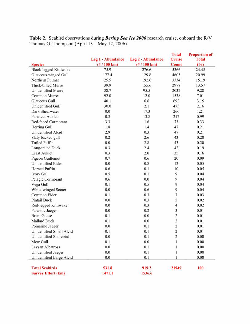
Table 2. Seabird observations during Bering Sea Ice 2006 research cruise, onboard the R/V Thomas G. Thompson (April 13 – May 12, 2006).

Leg 1 - Abundance Leg 2 - AbundanceTotal

CruiseProportion of

TotalSpecies (# / 100 km) (# / 100 km) Count (%)Black-legged Kittiwake 75.9 276.6 5366 24.45Glaucous-winged Gull 177.4 129.8 4605 20.99Northern Fulmar 25.5 192.6 3334 15.19Thick-billed Murre 39.9 155.6 2978 13.57Unidentified Murre 38.7 95.5 2037 9.28Common Murre 92.0 12.0 1538 7.01Glaucous Gull 40.1 6.6 692 3.15Unidentified Gull 30.0 2.1 475 2.16Dark Shearwater 0.0 17.3 266 1.21Parakeet Auklet 0.3 13.8 217 0.99Red-faced Cormorant 3.3 1.6 73 0.33Herring Gull 1.8 1.4 47 0.21Unidentified Alcid 2.9 0.3 47 0.21Slaty backed gull 0.2 2.6 43 0.20Tufted Puffin 0.0 2.8 43 0.20Long-tailed Duck 0.3 2.4 42 0.19Least Auklet 0.3 2.0 35 0.16Pigeon Guillemot 0.7 0.6 20 0.09Unidentified Eider 0.0 0.8 12 0.05Horned Puffin 0.6 0.1 10 0.05Ivory Gull 0.5 0.1 9 0.04Pelagic Cormorant 0.6 0.0 9 0.04Vega Gull 0.1 0.5 9 0.04White-winged Scoter 0.0 0.6 9 0.04Common Eider 0.1 0.3 7 0.03Pintail Duck 0.0 0.3 5 0.02Red-legged Kittiwake 0.0 0.3 4 0.02Parasitic Jaeger 0.0 0.2 3 0.01Brant Goose 0.1 0.0 2 0.01Mallard Duck 0.1 0.0 2 0.01Pomarine Jaeger 0.0 0.1 2 0.01Unidentified Small Alcid 0.1 0.1 2 0.01Unidentified Shorebird 0.0 0.1 2 0.00Mew Gull 0.1 0.0 1 0.00Laysan Albatross 0.0 0.1 1 0.00Unidentified Jaeger 0.0 0.1 1 0.00Unidentified Large Alcid 0.0 0.1 1 0.00

Total Seabirds 531.8 919.2 21949 100Survey Effort (km) 1471.1 1536.6

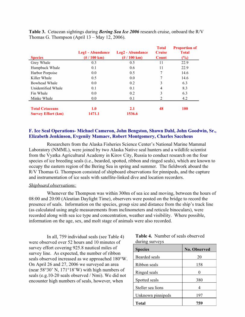
Table 3. Cetacean sightings during Bering Sea Ice 2006 research cruise, onboard the R/V Thomas G. Thompson (April 13 – May 12, 2006).

Leg1 - Abundance Leg2 - AbundanceTotal

CruiseProportion of

TotalSpecies (# / 100 km) (# / 100 km) Count (%)Grey Whale 0.3 0.5 11 22.9Humpback Whale 0.1 0.6 11 22.9Harbor Porpoise 0.0 0.5 7 14.6Killer Whale 0.5 0.0 7 14.6Bowhead Whale 0.0 0.2 3 6.3Unidentified Whale 0.1 0.1 4 8.3Fin Whale 0.0 0.2 3 6.3Minke Whale 0.0 0.1 2 4.2

Total Cetaceans 1.0 2.1 48 100Survey Effort (km) 1471.1 1536.6

F. Ice Seal Operations- Michael Cameron, John Bengston, Shawn Dahl, John Goodwin, Sr., Elizabeth Jenkinson, Evgeniiy Mamaev, Robert Montgomery, Charles Saccheus

Researchers from the Alaska Fisheries Science Center’s National Marine Mammal Laboratory (NMML), were joined by two Alaska Native seal hunters and a wildlife scientist from the Vyatka Agricultural Academy in Kirov City, Russia to conduct research on the four species of ice breeding seals (i.e., bearded, spotted, ribbon and ringed seals), which are known to occupy the eastern region of the Bering Sea in spring and summer. The fieldwork aboard the R/V Thomas G. Thompson consisted of shipboard observations for pinnipeds, and the capture and instrumentation of ice seals with satellite-linked dive and location recorders.

Shipboard observations:Whenever the Thompson was within 300m of sea ice and moving, between the hours of

08:00 and 20:00 (Aleutian Daylight Time), observers were posted on the bridge to record the presence of seals. Information on the species, group size and distance from the ship’s track line (as calculated using angle measurements from inclinometers and reticule binoculars), were recorded along with sea ice type and concentration, weather and visibility. Where possible, information on the age, sex, and molt stage of animals were also recorded.

In all, 759 individual seals (see Table 4) were observed over 52 hours and 10 minutes of survey effort covering 925.8 nautical miles of survey line. As expected, the number of ribbon seals observed increased as we approached 180°W. On April 26 and 27, 2006 we surveyed an area (near 58°30’ N, 171°18’W) with high numbers of seals (e.g.10-20 seals observed / Nmi). We did not encounter high numbers of seals, however, when

Table 4. Number of seals observed during surveysSpecies No. Observed

Bearded seals 20

Ribbon seals 158

Ringed seals 0

Spotted seals 380

Steller sea lions 4

Unknown pinnipeds 197

Total 759

we returned to the same area on April 29. (See the map observed and tagged seals in Figure 4 below.)

Captures and instrumentation:Capturing individual animals and instrumenting them with Satellite Data Recorders

(SDRs) was the primary objective of the ice seal project. SDRs transmit collected data to an overhead satellite, for later analyses. Two types of SDRs were used:

SPLASH tag – This tag collects information on the movements, dive and haulout behaviors of the instrumented animal. It is attached to the animal’s fur using marine epoxy and will fall off when the animal molts in June. As such, SPLASH data will only be available for 1-2 months after deployment.

SPOT tag – This tag only collects information on the movements and haulout behavior of the instrumented animal. It does not provide dive data and the transmission frequency is restricted to once each week to conserve battery life. SPOT tags are much smaller and lighter than SPLASH tags and are attached to a cattle ear tag which is then affixed to the inter-digital webbing of one of the seal’s rear flippers. As such, SPOT tags do not fall off with the molt and are programmed to transmit for at least 18 months before exhausting the battery.

While conducting shipboard observations, whenever a seal was seen in a location favorable for capture, (e.g. with a pup, in the middle of a large floe, on the edge of an ice finger), the ship was stopped to launch three Mark-III Zodiac inflatable rafts. Directed by an observer on the Thompson’s bridge, the three Zodiacs surrounded the seal. Researchers jumped onto the floe and, using long-handled nets, captured the seal. After physically restraining the seal, the SPLASH and/or SPOT tag(s) were attached, a tissue sample for DNA analysis was taken from the rear flipper, any scat or urine present on the floe was collected, and the seal’s length and girth were measured before releasing it.

Overall, 10 ribbon seals (5 adults: 5 pups), and 8 spotted seals (1 yearling: 7 pups), were captured and instrumented (see Table 5) at different locations throughout the study area (see Map). Shortly after deployment, all instruments were transmitting as expected. Researchers from NMML will continue to monitor the seals’ daily movements and dive behavior.

Table 5. Number of seals instrumented with different SDR types

Species Age Class Sex SPOT

onlySPLASH

onlySPLASH

and SPOT

RibbonPup M 3

F 2

Adult M 1F 2 2

Spotted Pup M 6F 1

Yearling F 1

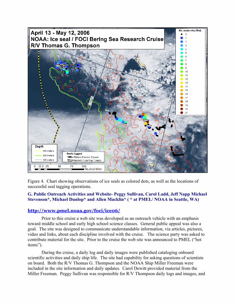
Figure 4. Chart showing observations of ice seals as colored dots, as well as the locations of successful seal tagging operations.

G. Public Outreach Activities and Website- Peggy Sullivan, Carol Ladd, Jeff Napp Michael Stevenson*, Michael Dunlop* and Allen Macklin* ( * at PMEL/ NOAA in Seattle, WA)

http://www.pmel.noaa.gov/foci/ice06/

Prior to this cruise a web site was developed as an outreach vehicle with an emphasis toward middle school and early high school science classes. General public appeal was also a goal. The site was designed to communicate understandable information, via articles, pictures, video and links, about each discipline involved with the cruise. The science party was asked to contribute material for the site. Prior to the cruise the web site was announced to PMEL (“hot items”).

During the cruise, a daily log and daily images were published cataloging onboard scientific activities and daily ship life. The site had capability for asking questions of scientists on board. Both the R/V Thomas G. Thompson and the NOAA Ship Miller Freeman were included in the site information and daily updates. Carol Dewitt provided material from the Miller Freeman. Peggy Sullivan was responsible for R/V Thompson daily logs and images, and

worked on the web site remotely from the ship. Allen Macklin, Michael Dunlap, and Mike Stevenson seamlessly accomplished land support for the site.

A number of classes followed the progress of our Ice-Edge Expedition using the Web site. Carol Ladd gave very-well received pre-and post cruise presentation about the cruise and our science activities to fifth- graders from four classrooms at an elementary school in Issaquah, WA. A Kodiak Island high school class visited the ship and the site before we left the dock. Carol Ladd and Jeff Napp, who joined the cruise for Leg 2, also gave presentations to 5th – 8th

graders at the St. Paul Island School on FOCI’s continuing studies of the Bering Sea ecosystem. A high school science teacher from Ohio reviewed the site in design phase, and his class also followed the cruise. The web site was well received by numerous science classes, and was also visited by friends and family of both the science party and the ships’ crew.

APPENDIX

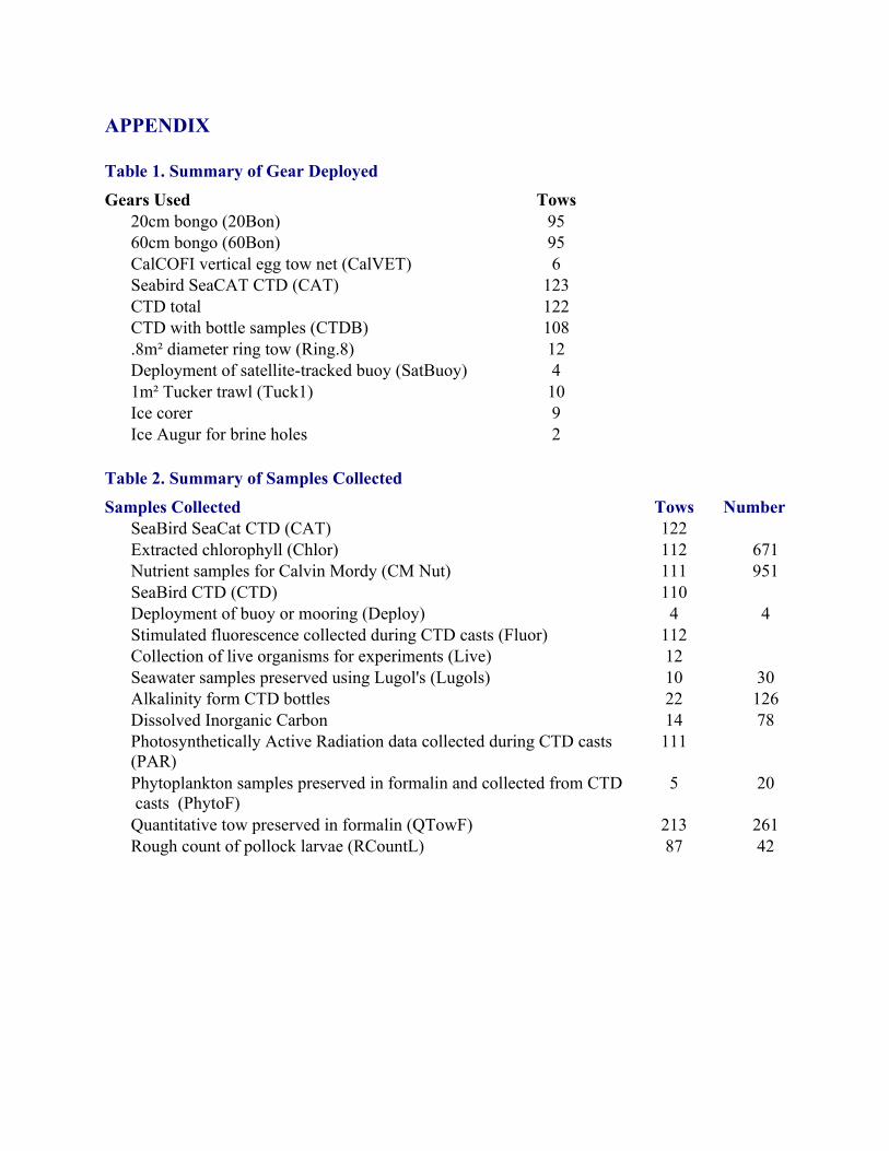
Table 1. Summary of Gear DeployedGears Used Tows

20cm bongo (20Bon) 9560cm bongo (60Bon) 95CalCOFI vertical egg tow net (CalVET) 6Seabird SeaCAT CTD (CAT) 123CTD total 122CTD with bottle samples (CTDB) 108.8m² diameter ring tow (Ring.8) 12Deployment of satellite-tracked buoy (SatBuoy) 41m² Tucker trawl (Tuck1) 10Ice corer 9Ice Augur for brine holes 2

Table 2. Summary of Samples CollectedSamples Collected Tows Number

SeaBird SeaCat CTD (CAT) 122Extracted chlorophyll (Chlor) 112 671Nutrient samples for Calvin Mordy (CM Nut) 111 951SeaBird CTD (CTD) 110Deployment of buoy or mooring (Deploy) 4 4Stimulated fluorescence collected during CTD casts (Fluor) 112Collection of live organisms for experiments (Live) 12Seawater samples preserved using Lugol's (Lugols) 10 30Alkalinity form CTD bottles 22 126Dissolved Inorganic Carbon 14 78Photosynthetically Active Radiation data collected during CTD casts 111(PAR)Phytoplankton samples preserved in formalin and collected from CTD 5 20 casts (PhytoF)Quantitative tow preserved in formalin (QTowF) 213 261Rough count of pollock larvae (RCountL) 87 42

INSERT EVENT LOG as Table 3