Crowd Textures5ptFrom Sensing Proximity to Understanding ... dissertation.pdf · conduct research and write papers, and most importantly making it a lot of fun. The support I received

Crowd TexturesFrom Sensing Proximity to Understanding Crowd Behavior

Claudio Martella

Ph.D. ThesisVrije Universiteit Amsterdam, 2017

This work was funded by the Dutch national program COMMIT/ underthe project P09 EWiDS.

This work was carried out in the ASCI graduate school.ASCI dissertation series number 364.

Usage of the painting “Exodus” on the cover is under kind permissionof artist Lesley Anne Cornish.

Manuscript printed by GVO.

ISBN 978-94-6332-140-2

Copyright © 2017 by Claudio Martella.

VRIJE UNIVERSITEIT

Crowd TexturesFrom Sensing Proximity to Understanding Crowd Behavior

ACADEMISCH PROEFSCHRIFT

ter verkrijging van de graad Doctor aande Vrije Universiteit Amsterdam,op gezag van de rector magnificus

prof.dr. V. Subramaniam,in het openbaar te verdedigen

ten overstaan van de promotiecommissievan de Faculteit der Exacte Wetenschappenop vrijdag 24 februarie 2017 om 11.45 uur

in de aula van de universiteit,De Boelelaan 1105

door

Claudio Martella

geboren te Bolzano, Italië

promotor: prof.dr.ir. M.R. van Steencopromotor: prof.dr.ir. H.E. Bal

Examiners:

prof.dr.ir. A. van Halteren VU University Amsterdam, Philips Researchprof.dr.ir. P. Havinga University of Twenteprof.dr. S. Klous University of Amsterdam, KPMGprof.dr. G.P. Picco University of Trentodr. S. Voulgaris VU University Amsterdam

To my mother.These days, nothing is in my head more than your words “You can do it.”

Well, those and “Stop picking your nose.”

Acknowledgements

A Ph.D. thesis is written to seem like the result of an unstoppable seriesof a-ha moments and eurekas. It could not be further from the truth.Pursuing a Ph.D. has felt more like “eating glass and staring into theabyss of death”, to quote Elon Musk talking about being an entrepreneur.Yet, regardless of the sweat, blood and tears, it has been a challengingand greatly rewarding journey I could not have completed without thehelp and support of many.

My first acknowledgments are certainly for my supervisor Maartenvan Steen, who took me on this journey when I had lost nearly all faithabout obtaining a Ph.D., and most of the hope about having a healthyand constructive relationship with a boss. Maarten has proven it notonly possible, but he has gone further by being a mentor and a modelthroughout these five years, teaching me with great passion how toconduct research and write papers, and most importantly making it alot of fun. The support I received during the hard hits in my career andpersonal life was much appreciated and will not be forgotten. I wouldalso like to thank Aart van Halteren for showing me that the industry canbe a place for science and research, often giving me novel and originalpoints of view and angles (for example, impressively predicting alreadyfive years ago I would end up working with beacons after my Ph.D.).Although we have not had the opportunity to do research together, Iwould like to thank Henri Bal for having my back (in particular when itwas injured) during my last years at the VU.

The next necessary acknowledgments go to my family, who also onthis journey has been by my side from start to end, by encouraging mydecision and supporting its execution. During these years we have beenthrough things nobody should have to, but we have shown our bond isstrong.

I want to continue by thanking my paranymphs Marco Cattani andKaveh Razavi for their job and for their friendship during these five

ix

years. You share positive attitude and a constant smile, together with anability to think out-of-the-box of which I am very jealous. A mention isdue for my paranymph honoris causa Ben Grass, who at times has copedwith some of my worst edges without ever breaking my nose (regardlessof his capability to do so – though everybody knows the liver punch ishis favorite shot). It is clear to me only now that you have introduced meto boxing only to have the opportunity to punch me repeatedly withoutany legal consequence.

A special notice of acknowledgment, or perhaps of blame, goes to EliaBruni and Matteo Caprari, who saw and nurtured the junior researcherthat was still in me during my years in the industry after obtaining myM.Sc., eventually being partially responsible for the choice to go backto academia for a Ph.D.

The work presented in this dissertation was conducted under theumbrella of the EWiDS project. The project and the work have broughtme to team up with a number of people from whom I have learnt greatand many things, like Claudine Conrado, Keon Langendoen, Jie Li,Andreas Loukas, Ioannis Protonotarios, and Marco Zuniga, to mentiona few. I feel lucky that my first years of work at the VU overlapped withthe last of Matthew Dobson, on whose work much of mine is based. Wehave had long days and weekends of hacking, and they were all fun. Aparticular mention is due for the long-lasting collaboration (technically,beginning three days before the official start of my contract – that shouldhave been a clear sign of what was about to happen to my life) withHayley Hung and Gwenn Englebienne, and later also with Ekin Gedikand Laura Cabrera-Quiros. The nearly masochistic way in which wepushed each other from a crazy experiment to the next is beyond myunderstanding.

I would also like to acknowledge the many people I have spent timewith at the VU, starting with the lovely colleagues I shared the officewith, including Rena Bakhshi, Albana Gaba, and Suhil Yousaf, whomanaged to make the long hours feel a bit shorter, continuing with thepeople with whom I shared many meals, coffees and borrels, includingSara Magliacane, Dirk Vogt (in this case, many cigarettes as well...),Lionel Sambuc, David van Moolenbroek, and Ismail Elhelw, and con-cluding with the secretaresses extraordinaire Caroline Waij and MojcaLovrencak, who were always there on a short notice to fix all the messwith my bureaucracy and so much more.

One of the reasons why it has been so gratifying to pursue a Ph.D.at the VU have been the opportunities of collaboration. I am glad for

x

the hours spent working with Ana Lucia Varbanescu, whose passion forteaching and research have opened my eyes about the fun and respon-sibilities that come with supervising students, and Alexandru Iosup’steam at TU Delft. The Lighthouse team meetings with Peter Bonczand Spyros Voulgaris have been something to look forward to. Thecollaboration for the CoBrA experiment with Jeana Frost has pushedme in the realms of the social sciences with positive surprises. I owecountless tokens of gratitude to Armando Miraglia for the number ofhours (and many extra hours) put in our projects. Your dedication andwork ethic is a continuous source of inspiration.

I would also like to acknowledge the many students I have had the plea-sure to work with who put effort, passion and great work in our projects,including Renske Augustijn, Christian Chilipirea, Jesse Donkervliet,Sinziana Filip, Unmesh Joshi, Ian Morozan, Per Ohme, Andreea Petre,Peter Rutgers, Andreea Sandu, Dimo Stoyanov, and Vlad Tudose.

I would like to extend my gratitude to Salvatore Scellato who enabledmy internship with the geo/beacons team at Google in London, UK,where I had the fantastic opportunity to apply some of my research in alegendary environment, and to the engineers I had the pleasure to workwith there, including Vilius Naudziunas, Stefano Maggiolo, NandanaDutt, Jonathan Morace, and the rest of the team.

I also had the pleasure to intern in the Big Data team at TelefonicaResearch in Barcelona, Spain, working together with the all-greek teamincluding Dionysios Logothetis, Georgos Siganos and Ilias Leontiadis,a collaboration that has been fruitful beyond the time boundaries of theinternship.

I am glad to acknowledge that, against common belief, the conceptsI learnt during my doctoral years are useful beyond the domain ofdistributed computer systems. For example, for a BBQ at the beach,one should buy disposable grills in excess. They can, and will fail.Redundancy is key. I have also learnt that in most cases a Ph.D. thesismanuscript is only used to raise the height of some computer screensor to level a table. For this reason, the cover of this manuscript isprinted on growth paper, meaning that it contains seeds of a mix ofwild flowers. Furthermore, the manuscript is printed on biodegradable100%-recycled paper. This way, the worst-case scenario where themanuscript is trashed in a backyard, or in nature in general, turns into amuch more desirable and colorful best-case scenario. Unfortunately, the“forget-me-not” flower seeds were not available.

xi

Finally, I would like to conclude with some apologies to Alan Turingand John von Neumann. In the acknowledgments of my B.Sc. and M.Sc.theses I gratefully noted that it was the work of the two scientists thatpushed me to decide to pursue a career in Computer Science. I alsosuggested, this time perhaps with a tiny note of blame, that my at-the-time status of single may be re-conducted to the very same decision.Well, maybe ironically, it was at the first conference in my doctoral yearsthat I met Vera, to whom I am grateful for her love and support, and forpushing me everyday out of my comfort zone. Jokes on me, I guess.

Claudio MartellaRio de Janeiro, Brazil, December 2016

xii

Publications

Design for Crowd Well-being: Needs and Design Decisions, J. Li, H.De Ridder, A. Vemeeren, C. Conrado, and C. Martella. In Proceedingsof the International Conference on Planning and Design (ICPD), 2013.

Design for Crowd Well-being: Current Designs, Strategies and Fu-ture Design Suggestions, J. Li, H. De Ridder, A. Vemeeren, C. Conrado,and C. Martella. In Proceedings of the International Association ofSocieties of Design Research (IASDR), 2013.

Crowd Textures as Proximity Graphs, C. Martella, A. van Halteren,M. van Steen, C. Conrado, and J. Li In IEEE Communications Magazine,2014.

How Well do Graph-Processing Platforms Perform? An EmpiricalPerformance Evaluation and Analysis Y. Guo, M. Biczak, A. Var-banescu, A. Iosup, C. Martella, and T. Willke. In Proceedings of theIEEE International Parallel and Distributed Processing Symposium(IPDPS), 2014.

Benchmarking Graph-Processing Platforms: A Vision, Y. Guo, M.Biczak, A. Varbanescu, A. Iosup, C. Martella, and T. Willke. In Pro-ceedings of the ACM/SPEC International Conference on PerformanceEngineering, Work-in-Progress (ICPE), 2014.

From Proximity Sensing to Spatio-Temporal Social Graphs, C.Martella, M. Dobson, A. van Halteren, and M. van Steen. In Pro-ceedings of the IEEE International Conference on Pervasive Computingand Communications (PerCom), 2014.

Adaptive Partitioning of Large-scale Dynamic Graphs, L. Vaquero,F. Cuadrado, D. Logothetis, and C. Martella. In Proceedings of theInternational Conference on Distributed Computing Systems (ICDCS),2014.

xiii

Spinner: Scalable Graph Partitioning in the Cloud, C. Martella, D.Logothetis, A. Loukas, and G. Siganos. In arXiv, 2014.

How Was It? Exploiting Smartphone Sensing to Measure ImplicitAudience Responses to Live Performances, C. Martella, E. Gedik, L.Cabrera-Quiros, G. Englebienne, and H. Hung. In Proceedings of theACM Multimedia Conference (MM), 2015.

Leveraging Proximity Sensing to Mine the Behavior of MuseumVisitors, C. Martella, A. Miraglia, M. Cattani, and M. van Steen.In Proceedings of the IEEE International Conference on PervasiveComputing and Communications (PerCom), 2016.

A Landscape of Crowd-Management Support: An Integrative Ap-proach, N. Wijermans, C. Conrado, M. van Steen, C. Martella, and J.Li. In Safety Science, 2016.

Powerful and Efficient Bulk Shortest-Path Queries: Cypher Lan-guage Extension & Giraph Implementation, P. Rutgers, C. Martella,S. Voulgaris, and P. Boncz. In Proceedings of the International Work-shop on Graph Data Management Experiences and Systems (GRADES),2016.

On Current Crowd Management Practices and the Need for In-creased Situation Awareness, Prediction, and Intervention, In C.Martella, J. Li, C. Conrado, and A. Vermeeren. In Safety Science, 2016.

Visualizing, Clustering, and Predicting the Behavior of MuseumVisitors, C. Martella, A. Miraglia, J. Frost, M. Cattani, and M. vanSteen. In Pervasive and Mobile Computing, 2016.

Exploiting Density to Track Human Behavior in Crowded Environ-ments, C. Martella, M. Cattani, and M. van Steen. In IEEE Communi-cations Magazine, 2017.

An Open-Space Museum as a Testbed for Popularity Monitoringin Real-World Settings, M. Cattani, I.Protonotarios, C. Martella, J.van Velzen, M. Zuniga, and K. Langendoen. In Proceedings of theInternational Conference on Embedded Wireless Systems and Networks(EWSN), 2017.

xiv

Contents

1 Introduction 11.1 Characterizing spatio-temporal proximity . . . . . . . 2

1.1.1 The spatial dimension . . . . . . . . . . . . . 31.1.2 The temporal dimension . . . . . . . . . . . . 4

1.2 Sensing modalities . . . . . . . . . . . . . . . . . . . 41.2.1 Tracking absolute location . . . . . . . . . . . 41.2.2 Tracking relative location . . . . . . . . . . . . 5

1.3 Proposed approach . . . . . . . . . . . . . . . . . . . 61.3.1 Crowds, crowd behavior, and crowd textures . 61.3.2 Problem statement . . . . . . . . . . . . . . . 8

1.4 Outline and contributions . . . . . . . . . . . . . . . . 9

2 On current crowd management practices and theneed for increased situation awareness, prediction,and intervention 112.1 Introduction . . . . . . . . . . . . . . . . . . . . . . . 112.2 Background . . . . . . . . . . . . . . . . . . . . . . . 132.3 Methodology . . . . . . . . . . . . . . . . . . . . . . 14

2.3.1 Participants . . . . . . . . . . . . . . . . . . . 162.3.2 Interview process . . . . . . . . . . . . . . . . 162.3.3 Data analysis . . . . . . . . . . . . . . . . . . 17

2.4 Findings . . . . . . . . . . . . . . . . . . . . . . . . . 182.4.1 Overview: on the definition of crowd management 192.4.2 Current practices . . . . . . . . . . . . . . . . 192.4.3 Limitations of current practices and crowd man-

agers’ requirements for the future . . . . . . . 282.5 Recommendations . . . . . . . . . . . . . . . . . . . . 31

2.5.1 Crowd management as two feedback control loops 322.5.2 Implications . . . . . . . . . . . . . . . . . . . 36

2.6 Discussion . . . . . . . . . . . . . . . . . . . . . . . . 372.7 Conclusions . . . . . . . . . . . . . . . . . . . . . . . 39

xv

3 Crowd textures as proximity graphs 413.1 Introduction . . . . . . . . . . . . . . . . . . . . . . . 413.2 Crowds and crowd dynamics . . . . . . . . . . . . . . 433.3 The proximity graph . . . . . . . . . . . . . . . . . . 44

3.3.1 Analyzing the proximity graphs . . . . . . . . 453.3.2 The awareness of the context . . . . . . . . . . 46

3.4 An instrument . . . . . . . . . . . . . . . . . . . . . . 483.4.1 Sensing technologies . . . . . . . . . . . . . . 493.4.2 System architecture . . . . . . . . . . . . . . . 503.4.3 A processing chain . . . . . . . . . . . . . . . 51

3.5 Real-world experiment . . . . . . . . . . . . . . . . . 523.6 Discussion . . . . . . . . . . . . . . . . . . . . . . . . 543.7 Conclusions . . . . . . . . . . . . . . . . . . . . . . . 57

4 From proximity sensing to spatio-temporal socialgraphs 594.1 Introduction . . . . . . . . . . . . . . . . . . . . . . . 594.2 Model . . . . . . . . . . . . . . . . . . . . . . . . . . 62

4.2.1 Problem definition . . . . . . . . . . . . . . . 624.2.2 Density-based clustering . . . . . . . . . . . . 644.2.3 K-nearest neighbors analysis . . . . . . . . . . 654.2.4 Proposed solution . . . . . . . . . . . . . . . . 66

4.3 Evaluation in simulation . . . . . . . . . . . . . . . . 664.3.1 Methodology . . . . . . . . . . . . . . . . . . 664.3.2 Setups . . . . . . . . . . . . . . . . . . . . . . 694.3.3 Results . . . . . . . . . . . . . . . . . . . . . 70

4.4 Evaluation in the real world . . . . . . . . . . . . . . . 754.4.1 Methodology . . . . . . . . . . . . . . . . . . 764.4.2 Evaluation against ground truth data . . . . . . 764.4.3 Evaluation at an ICT conference . . . . . . . . 77

4.5 Discussion . . . . . . . . . . . . . . . . . . . . . . . . 794.6 Related work . . . . . . . . . . . . . . . . . . . . . . 804.7 Conclusions . . . . . . . . . . . . . . . . . . . . . . . 81

5 Leveraging proximity sensing to mine the behaviorof museum visitors 835.1 Introduction . . . . . . . . . . . . . . . . . . . . . . . 83

5.1.1 Motivation . . . . . . . . . . . . . . . . . . . 855.2 Overview . . . . . . . . . . . . . . . . . . . . . . . . 87

5.2.1 Data-collection architecture . . . . . . . . . . 875.2.2 Data-filtering pipeline . . . . . . . . . . . . . 88

xvi

5.2.3 Data-analytics applications . . . . . . . . . . . 895.3 Related work . . . . . . . . . . . . . . . . . . . . . . 895.4 Model . . . . . . . . . . . . . . . . . . . . . . . . . . 91

5.4.1 Problem definition . . . . . . . . . . . . . . . 925.4.2 Particle filter . . . . . . . . . . . . . . . . . . 925.4.3 Density-based filter . . . . . . . . . . . . . . . 955.4.4 Majority-voting filter . . . . . . . . . . . . . . 96

5.5 Evaluation . . . . . . . . . . . . . . . . . . . . . . . . 965.5.1 Methodology . . . . . . . . . . . . . . . . . . 965.5.2 Results . . . . . . . . . . . . . . . . . . . . . 100

5.6 Visualizing visitor behavior . . . . . . . . . . . . . . . 1025.6.1 Artworks and rooms popularity . . . . . . . . 1025.6.2 Visitors common movement paths . . . . . . . 1035.6.3 Common positions of visitors . . . . . . . . . 1065.6.4 Artworks attraction and exhibition design . . . 1075.6.5 Focus group on visualizations’ effectiveness . . 108

5.7 Clustering visitor behavior . . . . . . . . . . . . . . . 1105.7.1 Time distribution across exhibits . . . . . . . . 1115.7.2 Clustering of paths . . . . . . . . . . . . . . . 112

5.8 Predicting visitor behavior . . . . . . . . . . . . . . . 1135.9 Discussion . . . . . . . . . . . . . . . . . . . . . . . . 1175.10 Conclusions . . . . . . . . . . . . . . . . . . . . . . . 118

6 Exploiting density to track human behavior in crowdedenvironments 1196.1 Introduction . . . . . . . . . . . . . . . . . . . . . . . 1196.2 Overview . . . . . . . . . . . . . . . . . . . . . . . . 120

6.2.1 Museum . . . . . . . . . . . . . . . . . . . . . 1206.2.2 Sensing infrastructure . . . . . . . . . . . . . 1226.2.3 Data analysis . . . . . . . . . . . . . . . . . . 124

6.3 Related work . . . . . . . . . . . . . . . . . . . . . . 1246.4 Model . . . . . . . . . . . . . . . . . . . . . . . . . . 126

6.4.1 Problem definition . . . . . . . . . . . . . . . 1276.4.2 Particle filter . . . . . . . . . . . . . . . . . . 1286.4.3 Smoothening . . . . . . . . . . . . . . . . . . 131

6.5 Evaluation . . . . . . . . . . . . . . . . . . . . . . . . 1326.5.1 Methodology . . . . . . . . . . . . . . . . . . 1326.5.2 Results . . . . . . . . . . . . . . . . . . . . . 134

6.6 Application . . . . . . . . . . . . . . . . . . . . . . . 1386.6.1 PoIs “popularity” over-time . . . . . . . . . . 1386.6.2 Crowd distribution across floors . . . . . . . . 139

xvii

6.6.3 Flows between floors . . . . . . . . . . . . . . 1396.7 Discussion . . . . . . . . . . . . . . . . . . . . . . . . 1406.8 Conclusions . . . . . . . . . . . . . . . . . . . . . . . 141

7 How was it? Exploiting smart phone sensing tomeasure implicit audience responses to live perfor-mances 1437.1 Introduction . . . . . . . . . . . . . . . . . . . . . . . 1437.2 Related work . . . . . . . . . . . . . . . . . . . . . . 1457.3 Case study 1: direct responses to a performance . . . . 147

7.3.1 Data collection . . . . . . . . . . . . . . . . . 1477.3.2 Feature extraction . . . . . . . . . . . . . . . 1497.3.3 Data analysis . . . . . . . . . . . . . . . . . . 1507.3.4 Classifying experience . . . . . . . . . . . . . 1517.3.5 Further analysis of salient moments . . . . . . 1557.3.6 Identifying sitting neighbors . . . . . . . . . . 157

7.4 Case study 2: impact of a performance on social behavior1587.4.1 Setup . . . . . . . . . . . . . . . . . . . . . . 1607.4.2 Results . . . . . . . . . . . . . . . . . . . . . 160

7.5 Discussion . . . . . . . . . . . . . . . . . . . . . . . . 1637.6 Conclusions . . . . . . . . . . . . . . . . . . . . . . . 164

8 Conclusions 1658.1 Summary of contributions . . . . . . . . . . . . . . . 1668.2 Limitations and future research . . . . . . . . . . . . . 167

Bibliography 171

xviii

1Introduction

„Deciding what to do is as important asdeciding what not to do.

— Steve Jobs

Zetabytes of user data are being collected every year, and the volumeis expected to grow more than linearly in the coming years. In the dataeconomy, data about our behavior on the Internet and the World WideWeb, including activities on social networking and social media sites, isused to compute, for example, search results, product recommendations,and news filters, not to mention to train the machine-learning modelsthat back smart features, and to improve user interfaces through A/Btesting.

The diffusion of smart phones has allowed us to interact with suchplatforms also when we are away from home, and their “apps” nowsupport many of our activities, resulting in even more data being pro-duced and collected. Today, smart phones are more powerful than thesupercomputers of 50 years ago, and they are packed with all sorts ofsensors and interaction interfaces. As such, they are in the privilegedposition to measure, together with our online activities, many aspects ofour offline behavior.

Smart phones and smart watches, and the upcoming wave of wear-ables, are opening a window in the digital world over our lives in thephysical one. And it appears to be just the beginning.

The number of ubiquitous and pervasive technologies is expectedto increase with the implementation of paradigms like the Internet ofThings, where all kinds of devices and appliances distributed around uswill be able to collect and share signals about our behavior. The process-ing of such signals with new machine-learning algorithms should finallyallow intelligent machines to predict, recommend, and personalize, tosupport our lives while receding in their background.

To manage all the data and applications we can leverage the infras-tructure built during the last decades, comprising reliable operating sys-tems, high-performance computing platforms equipped with application-

1

specific integrated circuits, large-scale distributed stores and queues,reliable and efficient cluster technology, as well as miniaturized, power-ful, and energy-efficient embedded devices.

Now, a larger attention needs to be put into finding the right signalsand the sensors to collect them, together with the right models andalgorithms to quantify and qualify our behaviors at massive scales. Mostimportantly, as many of our behaviors are social and the result of ourinteractions with the environment, in the future a particular emphasisis required on cohesive approaches that do not focus on the singleindividual or signal, but that take into account the collective, embodied,and situated nature of human behavior.

Spatio-temporal proximity is one signal, and it is the subject of thisdissertation.

1.1 Characterizing spatio-temporal proximity

As context shapes the meaning of a word in a sentence, objects andpeople around us define who we are and what we do. Due to thephysical constraints of our body and the ways we communicate, in thereal world we stand physically close to the objects and the people withwhom we interact. We face the people we talk to, we stand close to theappliances and objects we are using or need to reach, we share spaceswith co-workers and family.

Modeling and measuring spatial proximity, and how it develops overtime, is important for the understanding of human behavior.

Spatio-temporal proximity has been the object of extensive researchin recent years, from the identification of co-location in the workplace tothe characterization of face-to-face social interactions, to name two ex-amples. In its simplest form, proximity can be modeled as a relationshipbetween two entities, representing whether at a specific moment in timethe two entities were within a certain physical distance from each other.

This information can be further enriched, for example, by includingthe exact distance between the entities, the angle (e.g., if they are facingeach other), as well as a timestamp to encode the time when suchrelationship took place. While the information contained in a singleproximity relationship is simple and minimal, these dimensions, as wellas the possibly large number of relationships, allow for a number ofinteresting analyses.

Depending on the behavior to be measured and on the application,different variables of proximity information can be explored across

2 Chapter 1 Introduction

different dimensions, and they can be “zoomed” in and out to focus onmicro and macro aspects of the behaviors.

1.1.1 The spatial dimensionThinking about proximity, the first dimension that comes to mind, andperhaps the most intuitive, is the spatial dimension. Different ranges ofdistance can capture different aspects of social behavior. For example,interactions between individuals within 5-7 meters of distance relate tothe study of proxemics and the various kinds of spaces (e.g., personalspace, social space etc.), whereas longer ranges of distance up to around15 meters can be used to identify co-location in the study of cooperation(e.g., individuals sharing an office or part of an open space). In certainoccasions, one can even relate to, though perhaps not sense, longer rangegeographical proximity (e.g., kilometers of distance), as in the case ofthe study of cooperation within and between organizations on a territory.

Often, when focusing on a particular type of interaction or relationship,it is not necessary to measure the actual distance between the entitiesand a definition of a boundary or threshold can be enough. For example,it can be sufficient to capture proximity relationships that take placewithin a distance of 2-3 meters (without measuring the precise distance)to study f-formations1 and mingling behavior.

Furthermore, depending on the type of behavior, the angle of proxim-ity can determine the type of relationship or interaction. The most clearexamples are conversations and f-formations, which are characterized bya spatial and orientational relationship. To measure mingling behaviorand f-formations it is common to measure so-called face-to-face prox-imity, that is when individuals are facing each other within an angle ofsome 30-60 degrees at short distance. In contrast, for other behaviors,as in the case of crowd dynamics like clogging and pedestrian lanes, itis important to capture proximity across a more uniform space aroundthe individuals.

As with distance, it is not always necessary to characterize the actualangle of proximity between two individuals or between an individualand an object, but it is sufficient to capture whether the entities werewithin a certain maximum angle, as in the case of face-to-face proximity.

Different variables in the spatial dimension set different constraints tothe choice of modality and technology used to sense proximity.

1An F-formation arises whenever two or more people sustain a spatial and orientationalrelationship in which the space between them is one to which they have equal, direct,and exclusive access.

1.1 Characterizing spatio-temporal proximity 3

1.1.2 The temporal dimensionA proximity relationship can have a temporal property that defineswhen the relationship was valid. Different units of time can be used todetermine the duration of validity of a specific proximity relationshiplike, for example, a second. As in the case of the variables in the spatialdimension, also the unit of time is usually chosen depending on theunderlying behavior, and in particular the expected dynamicity or rateof change. For example, to identify co-location a time unit of someminutes may be enough, while for highly dynamic scenarios like crowddynamics one may need more fine grained time units, like seconds.

Clearly, the choice of time unit is influenced by the constraints dic-tated by the technology used to sense proximity, as higher samplingfrequencies tend to be more expensive to manage, for example, due tohigher battery consumption.

Furthermore, temporal properties can be used to aggregate a numberof proximity relationships over an interval of time (e.g., to filter andaggregate proximity relationships for a given day), in scenarios wherethe quantity of time spent in proximity is relevant to the study of thebehavior. Other examples of temporal aggregations are techniquesbased on sliding windows used, for example, to compute how proximitychanges over time. Finally, the temporal information can be used toinvestigate consequentiality, as in the case of the study of epidemics,where the temporal dimension is used to follow how information (ordiseases, mood, behavior etc.) spreads based on spatial proximity.

1.2 Sensing modalitiesThere is a number of different approaches and techniques to captureproximity, which can be divided in two groups.

1.2.1 Tracking absolute locationOn one hand, absolute location of individuals and objects is tracked atall times (e.g., as 3D or latitude-longitude coordinates), and proximityrelationships are captured by computing distances and angles (assumingone can also track who a person is facing) between these absolute coor-dinates, for example, through the Euclidean distance metric. Examplesof such approaches are video cameras, the Global Positioning System(GPS), and indoor localization systems (ILS). These approaches requiredeploying a fixed infrastructure as well as a mobile infrastructure, as


in the case of GPS and ILS where a device needs to be worn by theindividuals.

While techniques based on cameras do not need individuals to weara sensor, they tend to be less reliable when operating in challengingsettings with obstructions, changes in lighting conditions and requiringmerging multiple points of view. Furthermore, they are known to operatepoorly with high density of individuals, and need the deployment ofa large number of cameras to track large crowds. Finally, computer-vision algorithms tend to be compute-intensive and may cause concernsregarding the need to collect privacy-invasive footage.

Conversely, GPS and ILS techniques tend to be cheaper to computeand easier to anonymize (e.g., devices can be associated with unknownidentities for many applications), but still require the deployment of alandmark infrastructure that may be unfeasible to install at a scale atrequired granularity. Furthermore, GPS and ILS are also known to oper-ate poorly in high-density conditions, and usually provide localizationerrors of some meters in the best case. Finally, the capturing of angleof proximity often depends on additional sensing modalities, as, forexample, through the use of a compass.

1.2.2 Tracking relative location

On the other hand, relative location of individuals and objects is trackedas binary proximity relationships, with the only information that isrecorded being whether two entities, including individuals, objects, andpoints-of-interest, were close to one another (hence, relative) at a giventime. Like GPS and ILS systems, this approach requires individuals andobjects to be instrumented, but this time the sensors must detect othersensors only within a certain distance and angle.

The advantage of this approach is a limited dependency, if any, onfixed infrastructure and landmarks, as no intermediate step of absolutelocalization is necessary. Furthermore, this approach is particularlyadvantageous as sensors can be installed at and worn only by entitiesof interest, and the detection of proximity between two entities dependssolely on the two sensors involved. This way, it is simpler to deploy alarge-scale network of proximity sensors, with fewer centralized compo-nents, and sensors can be added only where and when needed, makingthis approach suitable to real-world dynamic deployments both outdoorsand indoors (e.g., in festivals, city events, but also in museums, trainstations etc.).

1.2 Sensing modalities 5

Typical technologies used to implement proximity sensors are radio-based (e.g., Bluetooth low-energy (BLE) and Zigbee), ultrasound, andinfra-red sensors, where a unique identifier can be transmitted and re-ceived within a certain distance range. Angles of detection can beenforced either by means of directional antennas, or by leveraging theshielding effect of the body of the individuals when the sensor is worn,for example, on the chest. Recently the industry has provided someattempts of standardizing a protocol for proximity sensing through smalland inexpensive BLE transmitters and BLE-enabled receivers (e.g.,smart phones and smart watches). Examples of such efforts are Apple’siBeacon and Google’s Eddystone.

1.3 Proposed approachThe work I present in this dissertation follows the second approach ofcapturing and modeling social behavior by leveraging relative-proximityinformation, and in particular by means of radio-based proximity sen-sors.

The main research question around which this work develops regardswhether social behavior can be measured with proximity sensors, andwhether by analyzing proximity data one can gain a better understandingof the measured behavior, and produce insights and feedback to ensurethe safety and comfort of a crowd.

1.3.1 Crowds, crowd behavior, and crowd texturesSocial behavior is a loose term that is intentionally used in this dis-sertation to refer to a wide range of behaviors involving a number ofindividuals. Proximity information can be used to study a large numberof different social behaviors in a variety of contexts and applications thatrange from the patterns emerging in a crowded place, the interactions ina workplace, the dynamics developing in a large city, to the foundationsof other technologies like the Internet of Things, to name a few examples.However, it is outside the scope of this dissertation to characterize anddefine all of them.

Instead, I focus on one instance, that is crowds and crowd behavior.The term crowd is used to refer to a large number of individuals, and

it can be characterized differently depending on the object and fieldof study. In this dissertation, I use the term to refer to a number ofindividuals gathering in the same place over a well-defined period oftime, which can last from hours to days, with all members not necessarily


being in that same place at the same time, nor necessarily sharing thesame goal or interest.

Such definition fits crowds gathering at train stations, music festivals,museum exhibitions, city parades etc., and it differs from definitionsof crowds where a number of individuals are dislocated and distributedgeographically in very different places and may never be in the sameplace at the same time (e.g., when one wants to study the profile andbehavior of customers of some coffee chain or the means and patternsof commute in a city, like in mobile crowd sensing studies).

Crowd behavior can be characterized according to a number of differ-ent aspects, all related to proximity information.

First, there are purely spatio-temporal aspects, as in the case of so-called crowd dynamics, which refer to bi-directional pedestrian lanes,flows, queues, clogging and congestions, etc. Second, there are moresocial aspects of crowd behavior, where related and interacting indi-viduals spend time close to each other, for example, while mingling orotherwise. Third, there are other aspects regarding relationships betweenindividuals with respect to profile, taste, and behavior, which can becharacterized by how similar people tend to distribute their time in asimilar way not only with other people, but also at certain places andinteracting with certain objects. Finally, there are higher-level aspects ofcrowd behavior that include, for example, emotions, moods, and actions,which are more suited to be studied by means of other types of sen-sors (e.g., microphones, accelerometers, video cameras, galvanic skinresponse sensor, etc.), but where proximity information can still play arole, for example, to study how these elements spread in the crowd.

In this dissertation, I argue that it is not possible to understand thebehavior of a crowd by focusing on the behavior of the single individualsin isolation.

In fact, similar to a flock of birds, the behavior of the individuals in acrowd can be understood only if their nearby individuals are taken intoaccount. Note that objects and points-of-interest can act as proxies toextend the definition of nearby, by allowing to relate individuals thatwere at the same place at different moments (e.g., in front of a painting,in a bar, in a specific room). This notion of dependency on nearbyindividuals creates a recursive relationship, where the members of acrowd are interleaved by a series of proximity relationships.

I coined the term crowd texture to refer to the series of interleavedproximity relationships characterizing a crowd and its behavior.

1.3 Proposed approach 7

I also argue that different crowd behaviors are characterized by differ-ent crowd textures (or that different crowd behaviors affect the crowdtexture in a different way), and that by mining the series of measuredproximity relationships crowd behaviors can be recognized and identi-fied. While, intuitively, one can think of recognizing crowd behaviorin the texture of a crowd as performing pattern matching on a series ofspatio-temporal proximity relationships, in practice, a broad range ofdata-analysis algorithms and techniques can be used.

Crowd textures, and the so-called proximity graphs used to representthem, are the elements that bind together the chapters of this dissertation.

1.3.2 Problem statement

Answering the research question presented in this dissertation requiresfinding a solution for the following problems.

• Current crowd-management practices and tools are lacking cer-tain information and capabilities, which existing technologies areunable to provide or fail to provide in certain conditions. We wantto understand, pulling directly from the professionals operatingon the field, requirements and needs of crowd managers to helpthem manage safer and more comfortable crowds.

• It is not clear what are the properties and limitations of relativelocalization, and how such type of information can be leveraged tomodel and identify crowd behavior. We want to identify effectivemodels to represent the texture of a crowd, starting from proximityinformation, that can enable the identification of the underlyingcrowd behaviors and dynamics.

• Sensing relative proximity with radio-based sensors is unreliabledue to the inherent limitations of wireless sensors networks andradio-based communication. We want to design an architecture ofa system to collect proximity information in the real-world thatcan operate in the face of the challenges dictated by scale, density,and extreme environmental conditions.

• Once a reliable measurement of a crowd texture is performed, it isnot clear how to analyze it to identify, quantify, or qualify the un-derlying crowd behaviors. We want to design a set of algorithms,without assuming a perfect and complete measurement, to under-stand what is happening in the crowd. Moreover, the algorithmsshould operate in respect of the privacy of the members of thecrowd.


• Identifying and characterizing crowd behavior are the first stepstowards ensuring the safety and comfort of a crowd. We wantto study strategies to gain insights and turn them into actionableinformation. This may comprise feedback to the crowd managersand/or to the crowd.

• Finally, proximity information has its limitation, perhaps missinghigher-level aspects of crowd behavior. We want to understandhow proximity information can work in cooperation with othersensing modalities to study the facets of crowd behavior that relatemore with the inner experience of the individuals.

1.4 Outline and contributions

This dissertation tries to tackle the above problems and makes the followcontributions.

In Chapter 2, we study current crowd management practices by meansof ten interviews conducted with professionals managing some of thelargest crowds in The Netherlands. Needs and requirements are identi-fied, including the limitations of current approaches and technologies.In particular, the interviewees reported a strong need for increased situa-tion awareness, prediction, and intervention, positioning spatio-temporalaspects of crowd behavior, like density, flows, and congestions, at thetop of their priorities. Recommendations are provided within the frame-work of a techno-social system for crowd management comprising twofeedback-control loops.

In Chapter 3, we dive into the definitions and properties of crowd tex-tures and proximity graphs. Examples of analyses to identify pedestrianlanes, bottlenecks, and social groups are provided, along with a discus-sion about the importance of taking into account the context arounda crowd, as well as advantages of instrumenting objects as well as in-dividuals with proximity sensors. A real-world use case is presented,by identifying social groups within face-to-face proximity from datacollected during an ICT conference.

In Chapter 4, we analyze some of the sources of unreliability inmobile and fixed proximity sensing when applied to crowd monitoring.A filter with a few parameters, and a technique to choose good valuesfor them, is presented and evaluated both in simulation and in a numberof real-world experiments. The technique can double the sensitivity ofthe measurement, reconstructing nearly all missed proximity detectionsand ignoring spurious ones.

1.4 Outline and contributions 9

In Chapter 5, we focus on tracking an indoor crowd inside a museum,studying in particular person-to-object face-to-face proximity relation-ships. A pipeline of filters is presented, comprising a particle filteradapted to directional sensing, together with a number of applicationsto visualize, cluster, and predict the behavior of the museum visitors,with data collected during a real-world 5-days experiment conducted atthe CoBrA museum of Amsterdam. We also look into the results of anumber of interviews and a focus group conducted with museum staffregarding the effectiveness of the visualizations.

In Chapter 6, we look into an extension of the previous techniquethat takes into account also person-to-person proximity, to overcomelimitations caused by high densities. The technique is evaluated during alarge-scale experiment with nearly a thousand participants conducted atthe NEMO museum, a particularly challenging setup due to the peculiarfeatures of the NEMO building. Together with the filtering pipeline,an analysis to detect crowded events as well as flows between floors ispresented.

In Chapter 7, we study how proximity sensors can be used togetherwith accelerometers to study the response of a crowd to a dance per-formance. An experiment is presented where audience behavior wastracked before, during, and after the performance, to try to identifythe response of the audience (e.g., enjoyment) by looking into the col-lective movements of the (seated) audience during the performance,and the differences in mingling behavior exhibited before and after theperformance.

The dissertation terminates with a brief discussion and conclusions.


2On current crowd managementpractices and the need forincreased situation awareness,prediction, and intervention

„If the user can’t use it, it doesn’t work.

— Susan Dray

2.1 IntroductionIn the previous chapter we have discussed how spatio-temporal informa-tion can help the study of social behavior. We have also specified theparticular focus of this dissertation on crowd behavior as one instanceof social behavior. To begin the work, in this chapter we first focuson gaining a better understanding of the state-of-the-art practices andtechnologies used by the professionals that work with crowds and theirbehavior on a daily basis, that is crowd managers.

Crowd management is essentially a set of collaborative practices be-tween a number of different actors, e.g., event planners and managers,emergency services, local authorities, transport authorities, stewards,and the crowd itself [29, 148]. These practices start months ahead ofan event. In fact, as we discuss in this chapter, preparations take about90% of the efforts. Usually a multi-agency approach is followed, in-corporating all relevant parties, to enable a wide range of knowledgeand expertise to be drawn upon. Preparation activities include detailedrisk analyses to identify and prioritize potential risks, use and develop-ment of comprehensive “what-if” scenarios to consider managementstrategies and contingency plans, establishment of a control point to

The contents of this chapter have been originally published in “On current crowdmanagement practices and the need for increased situation awareness, predic-tion, and intervention” C. Martella, J. Li, C. Conrado, A. Vermeeren - SafetyScience 2016, and have been slightly modified to improve readability.

11

coordinate all activities and personnel. The remaining 10% consists ofimplementing the plan, comprising monitoring crowd activity to identifypotential problems, and intervention, that in extreme conditions canresult in crowd control. It must be noted that the focus of crowd man-agement is facilitating crowd activities, hence proactively preventing, orquickly resolving, problems. The correct and effective execution of suchpractices is crucial to the success of an event, with the most importantoutcome being the safety and comfort of the crowd [2, 51].

It has been argued that a more systematic approach to crowd manage-ment could have avoided recent accidents in large crowded events [41,28]. We postulate that new developments in technology, including mo-bile sensors, decision-support systems, and novel communication andinteraction paradigms, can support crowd management operations dur-ing the planning and implementation of an event. However, as alsosupported by our results, currently the success of operations is stillmainly dependent on the personal experience and skills of the crowdmanagement team, with little or no aid from technology.

Towards a better understanding of the limitations and requirementsof current crowd management practices, in particular regarding the roleof technology, we present the perspective of crowd managers. We inter-viewed 10 crowd managers daily involved with managing large crowds,including a stadium hosting tens of thousands of visitors, a large trainstation, a multi-day music festival, a yearly celebration involving morethan a million people. A main result emerging from our interviews isthat crowd managers feel the need for instruments offering an increasedsituation awareness, a more reliable and timely monitoring of the stateof the crowd, and the ability to predict and steer the behavior of thecrowd without use of force.

In this chapter, we make the following contributions. First, we presentbackground and supporting literature, including crowd behavior model-ing and prediction, mobile sensing, and decision-support systems. Sec-ond, we present current crowd management practices, as they emergedduring our interviews. In particular, we focus on the role of technologyand its limitations. Third, we present crowd managers’ requirements forfuture technology to support their operations. Finally, we discuss oppor-tunities and recommendations within the framework of a techno-socialsystem.

12 Chapter 2 On current crowd management practices and the need for

increased situation awareness, prediction, and intervention

2.2 BackgroundA generally accepted definition of a crowd is that it is a large gatheringof diverse people at the same physical location, at the same time, notnecessarily sharing the same goal or interest [147]. Understandingthe behavior of crowds, and how to manage them effectively, is still ascattered effort that involves different fields including theoretical physics,sociology, psychology, computational science, and artificial intelligence.Recently, studies have been published with overviews of common crowdmanagement practices [29, 65], but more work is required. The literatureabout crowds and crowd behavior focuses on theoretical modeling of thepsychology of crowd behavior [126, 117], predicting crowd behaviorthrough physics-inspired models, recognizing behaviour through variouskinds of sensors and analysis.

An approach to studying crowd behavior is by synthesizing it throughcrowd behavior prediction models. Crowd behavior prediction modelsare also used for a-priori planning of events through simulation [132,165, 7, 125]. A popular example of a crowd behavior model is thesocial-force model [67]. The models usually target so-called crowddynamics, referring to patterns of crowd movement, and more preciselyto “the coordinated movement of a large number of individuals to whicha semantically relevant meaning can be attributed, depending on therespective application” [120]. Examples include a queue of people, theformation of uni-directional “lanes” in bi-directional pedestrian flows,the intersection of these lanes, or a group of people at a specific location.Approaches to crowd modeling and simulation have been extensivelysurveyed [139, 15, 48].

A different approach is to investigate how to detect and recognizecrowd behavior. Computer-vision techniques have been employed tocharacterize and automatically detect anomalies in a crowd [166, 161].The diffusion of pervasive and ubiquitous technologies such as smartphones and smart watches, has enabled the monitoring of social behav-ior through a wide range of sensing modalities, from temperature, tomovement, to spatial proximity [141, 11]. For example, smart phoneshave been used to detect crowd dynamics such as pedestrian flows andbottlenecks, and social groups [153, 154, 156]. In particular, crowddynamics such as pedestrian lanes and clogging have a strong spatio-temporal nature that can be captured as so-called crowd textures usingproximity sensors [97] (see Chapter 3). Accelerometers can be used tocharacterize queues, and activities such as running and walking [83].Finally, microphones can be used to measure the mood of a crowd [33]

2.2 Background 13

or recognize locations and places [84]1. Some of these approaches aregrouped also under the term Ambient Intelligence (AmI), referring to“electronic systems that are sensitive and responsive to the presenceof people” including context and social-aware miniaturized pervasivecomputing devices and sensors, which can be envisioned to enhance andsupport, for example, crowd monitoring and evacuation [104].

While synthesizing and recognizing crowd behavior has been ad-dressed in the literature, less attention has been dedicated to how suchdata can help crowd managers make effective decisions in the controlroom, for example, during an event. Existing works either tend to focuson managing disasters and emergencies [23, 111, 92, 114, 10, 73], oron very specific cases such as air traffic control [17, 95] and under-ground stations [134, 93], overlooking how technology can be used tosupport decisions before accidents happen during an event, or to supportplanning and debriefs.

Theories on socio-technical systems recommend new systems to bedesigned and operated with a holistic approach that optimizes bothtechnical and social factors [31, 30, 35, 34]. This body of work is crucialto the design of systems that make use of technology to support the workof crowd managers. While these principles have been applied to thedomain of technology and work design over the last decades, a broaderand braver approach is necessary to extend their reach, for example,to crowd management [40]. In this chapter, we take a technologicalstand within this attempt, by studying how technology currently helps(or fails to help) crowd managers in their practices, and how existingand new research can serve the work of crowd managers in organizingand managing safer and more secure crowds.

2.3 Methodology

In this section we present our participants and the methods used toconduct the interviews and analyze the collected data.

1Note that these techniques differ from the emerging field of Mobile Crowd Sensing(MCS) [60]. MCS uses mobile devices to collect information from individualsdislocated and distributed in wide areas, and defines a crowd as a large number ofindividuals that may be distributed geographically in different locations (and evendifferent countries), or that visit the same location at different times.



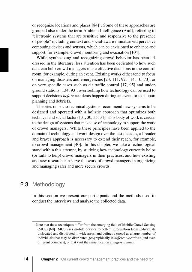
Crowd expert Description Crowd size Crowd durationP1 Indoor Music Festival Chief organizer of an annual indoor music festival, coordinating the

preparation, registration, staff training, communication during the festi-val

2000 6 hours

P2 Indoor Conference Chief organizer of an annual large indoor conference, coordinating theregistration, communication, transportation, parking, catering etc.

1000 12 hours

P3 Central Train Station Crowd manager of a central train station in a capital city, managing thecrowds in daily situations and in large events

250.000 4 hours

P4 Police Crowd manager involved with large crowds e.g., on a national festival 700.000 8 hoursP5 Security Company Head of a security company, consulting on organization and manage-

ment of various crowd events1000-100.000 hours to days

P6 Barrier Company Head of a barrier company designing and building custom barriers forvarious types of crowd events as well as managing their layout

1000-100.000 hours to days

P7 Outdoor Music Festival Manager of an annual outdoor music festival, coordinating the siteconstruction, ticketing, crowd flow control, transportation, parking,catering etc.

60.000-100.000 3 days

P8 Stadium Crowd manager of a stadium, managing the crowds for various events,such as concerts and football matches

55.000 4-5 hours

P9 Theme Park Manager of a theme park,focusing on managing the daily crowd flows,queues and large crowds (e.g., crowds watching a music fountain)during holidays

40.000-60.000 12 hours

P10 Train Station Flow Crowd manager of a central train station, monitoring real-time crowdflows via video cameras, Bluetooth and Wi-Fi signals

180.000 12 hours

Tab. 2.1 Description of the experts interviewed.

2.3.1 Participants

We carried out 10 individual interviews with 10 crowd experts. Weselected and approached 10 organizations in The Netherlands known forhosting and managing among the largest crowds in the country. Fromeach organization, we interviewed a senior professional with experiencein dealing with large crowds. Type of event, location, visitors profiles,time of year, among others, define different scenarios of crowd behaviorand the different strategies to manage them. For this reason, we choseorganizations that allowed us to cover the widest range of events andcrowds, from those emerging at peak hours in train stations to thosein multi-day outdoor music festivals. Note that also within the sametype of location, e.g., a train station, experts manage diverse scenarios.For example, train stations must deal with both week-day peak-hourscrowds and day-long special celebration events, with hundreds of thou-sands of people coming in from all over the country. We summarizethe participants and their domain of expertise in Table 2.1. We alsoincluded an expert from the Research & Development department ofan organization specialized in designing and building barriers for largeevents, such as music festivals and parades. As such, he presented adifferent perspective of the requirements and the use cases of the crowdmanagers. Finally, the organization we dubbed “Security Company”differs from the other organizations due to their consultancy-orientedbusiness model, that includes the delivery of crowd management train-ings and workshops, as well as consulting on events organization andmanagement. While diverse, the profile of the crowds managed by theparticipants matches our definition of a crowd provided above, that is ofa large number of individuals gathering at the same location at the sametime [147].

2.3.2 Interview process

We chose to conduct semi-structured interviews because they guaranteeconsistency in the topics that were addressed, but also freedom for theparticipants to diverge and provide their unique and personal perspectivewhen necessary. The approach prevented interviews falling into a strictquestion-response pattern and encouraged the raise of theme-relatednew questions that can adequately elicit the issues to compose a morecomprehensive report. Each interview was scheduled around 1 to 1.5hours at the work place of the participant, and it was recorded with avoice recorder. All the artifacts accessed in the interviews, for example,



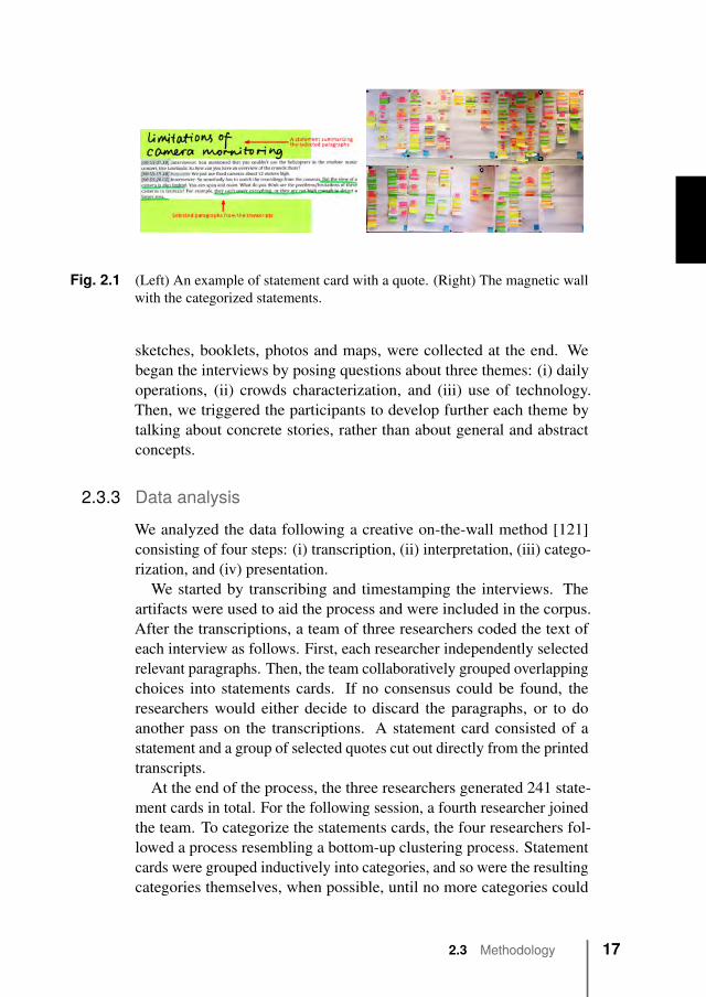
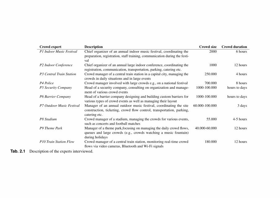
Fig. 2.1 (Left) An example of statement card with a quote. (Right) The magnetic wallwith the categorized statements.

sketches, booklets, photos and maps, were collected at the end. Webegan the interviews by posing questions about three themes: (i) dailyoperations, (ii) crowds characterization, and (iii) use of technology.Then, we triggered the participants to develop further each theme bytalking about concrete stories, rather than about general and abstractconcepts.

2.3.3 Data analysisWe analyzed the data following a creative on-the-wall method [121]consisting of four steps: (i) transcription, (ii) interpretation, (iii) catego-rization, and (iv) presentation.

We started by transcribing and timestamping the interviews. Theartifacts were used to aid the process and were included in the corpus.After the transcriptions, a team of three researchers coded the text ofeach interview as follows. First, each researcher independently selectedrelevant paragraphs. Then, the team collaboratively grouped overlappingchoices into statements cards. If no consensus could be found, theresearchers would either decide to discard the paragraphs, or to doanother pass on the transcriptions. A statement card consisted of astatement and a group of selected quotes cut out directly from the printedtranscripts.

At the end of the process, the three researchers generated 241 state-ment cards in total. For the following session, a fourth researcher joinedthe team. To categorize the statements cards, the four researchers fol-lowed a process resembling a bottom-up clustering process. Statementcards were grouped inductively into categories, and so were the resultingcategories themselves, when possible, until no more categories could

2.3 Methodology 17

Fig. 2.2 The hierarchy of categories generated by the bottom-up clustering of the state-ments. Each category further contains common themes emerged during theinterviews.

be generated or grouped. Figure 2.2 presents the first two levels of thehierarchy of categories, which we use to present our results in Section2.4. The clustering was not directed by any pre-defined hypothesis,and each category name emerged during the process. The session wascarried out in a room with walls covered by magnetic white boards. Adozen of A1 white paper sheets were fixed on the wall with magnets.The statement cards with relevant information were put together on thesame A1 sheet. Figure 2.1 shows an example of a statement card and apart of the magnetic wall.

The findings were presented in the form of a poster2. As we discussin the next session, time is an important dimension in the managementof crowds. For this reason, the visualization is constructed around atime-line. The poster visualizes the categories together with the mostimportant statements. Interesting quotes are printed with larger fontsizes to guide the attention towards the more detailed summaries. Wepresent a detailed analysis of the results in the next section.

2.4 FindingsIn this section we present our findings, organized following the hierarchyof categories pictured in Figure 2.2, emerged from the data analysispresented in Section 2.3.

2The poster can be downloaded from https://goo.gl/O38B9F



https://goo.gl/O38B9F

2.4.1 Overview: on the definition of crowd management

All experts strongly emphasized two main distinctions during the in-terviews. The first distinction related to the difference between crowdmanagement and other practices like crowd control and riot control.The second distinction related to the two phases that constitute thecrowd management practices, namely what happens before the eventand what happens during the event. We organize our findings aroundthese distinctions.

Crowd management is usually defined as the set of measures takenin the normal process of facilitating the movement and enjoyment ofpeople [18], for instance measures to control the distribution of peopleover a certain area. This definition fits that of the interviewees. Fromtheir responses, crowd management is taken to refer mostly to the prepa-rations for a given event and it involves predicting what is going tohappen and preparing for it, i.e., designing for the desired behavior ofthe crowd. The preparations involve all aspects, namely getting peopleinto the site, people participating to the event, and getting people outof the site. These preparations usually start much ahead of the event,e.g., six months or more. The resulting plan or design for a given eventconcerns the technical infrastructure and operational measures neededfor the safety, well-being and enjoyment of the crowd. The effort toproduce the plan was estimated by the interviewees to be about 90%of the total effort for the event’s crowd management. The remaining10% refers to the (mostly) operational measures, including potentiallyemergencies during the event itself, which implement and support theplan for the event.

Crowd management was distinguished from crowd control. The latterincludes all measures taken once crowds are beginning to or have goneout of control. In other words, crowd management is proactive whilecrowd control is reactive [18]. This distinction is reflected both by theuneven allocation of resources towards preparation, and by an emphasisof monitoring, predicting, and steering behavior during the event to avoidthe need for crowd control. In this chapter we focus in particular oncurrent practices, limitations and requirements of crowd management.

2.4.2 Current practices

We start by presenting current practices. Where not specified, crowdmanagers did not mention use of technology, or explicitly reported none.

2.4 Findings 19

Preparation: 90% of the efforts Execution: 10% of the efforts

Build-up phase Event Break-up

phase

Understanding visitors profilesConsidering the location

Managing the clientsCooperating with the institutions

Choosing the personnel

Logistical plan Action plan

Accounting for the event typePreparing for the weather

Managing build-up and break-upControlling flows, bottlenecks and queues

Ensuring constant communication

Continuous monitoring of the crowdPredicting and preventing accidents

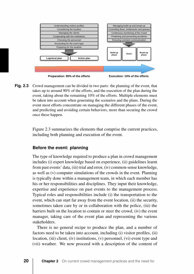
Fig. 2.3 Crowd management can be divided in two parts: the planning of the event, thattakes up to around 90% of the efforts, and the execution of the plan during theevent, taking about the remaining 10% of the efforts. Multiple elements mustbe taken into account when generating the scenarios and the plans. During theevent most efforts concentrate on managing the different phases of the event,and predicting and avoiding certain behaviors, more than securing the crowdonce these happen.

Figure 2.3 summarizes the elements that comprise the current practices,including both planning and execution of the event.

Before the event: planning

The type of knowledge required to produce a plan in crowd managementincludes (i) expert knowledge based on experience, (ii) guidelines learntfrom past events’ data, (iii) trial and error, (iv) common-sense knowledge,as well as (v) computer simulations of the crowds in the event. Planningis typically done within a management team, in which each member hashis or her responsibilities and disciplines. They input their knowledge,expertise and experience on past events to the management process.Typical roles and responsibilities include (i) the transportation to theevent, which can start far away from the event location, (ii) the security,sometimes taken care by or in collaboration with the police, (iii) thebarriers built on the location to contain or steer the crowd, (iv) the eventmanager, taking care of the event plan and representing the variousstakeholders.

There is no general recipe to produce the plan, and a number offactors need to be taken into account, including (i) visitor profiles, (ii)location, (iii) client, (iv) institutions, (v) personnel, (vi) event type and(vii) weather. We now proceed with a description of the content of



the crowd management plan, and later in this section we describe theaforementioned factors in detail.

The planning starts with a definition of the desired behavior the crowdmanagement team wants to obtain from the crowd. The content of theplan is the outcome of all the decisions that should eventually steerthe crowd towards that desired behavior during the event. Such plan isgenerally composed of two parts.

The first part is a logistical plan that concerns decisions about, forexample, the number of tickets sold, the mobility plan and the resultinglayout of the event site including the position of barriers, entrances,exits, toilettes, bars, the transportation systems, the provisioning offood and beverages. The main goal of these decisions is to allow thecrowd to move freely and safely, but at the same time avoid certaindangerous or unpleasant situations caused, for example, by unevendistribution of the crowd, obstructions, bottlenecks, and dissatisfaction.Communication with the crowd is also taken into account. Hence,the plan includes decisions, for example, about signs, screens, eventprogram, and maps. Additionally, the plan contains information aboutthe number of individuals in the personnel and their profiles, includingtheir protocols and briefings.

The second part resembles an action plan which consists of a numberof “what-if” scenarios and strategies regarding how to respond to eachgiven situation. This includes the preparation of scenarios for severalalternative “normal” situations, depending on weather, type of public,locations, most likely crowded areas, peak hours, as well as for deal-ing with emergencies, including evacuation plans and crowd control.Scenarios are typically constructed with the help of expert knowledgeand computer simulations, and the planning also indicates the coursesof action that may be taken in the given situation. Critical scenariosin events involving large crowds are the arrival and departure of thepeople at and from the site, so special attention must be paid for thepreparations for these moments.

Understanding the visitors is the first step in event planning. All theplanning for an event has to be adapted to its visitor profiles. The age andgender of the visitors are of great importance. It is easy to imagine thatyoung, aggressive and male adults in football stadiums are more difficultto manage than less active and well-behaved older adults. The visitors’familiarity or former experience of an event also plays an influential role.For example, it is common to see loyal visitors to some annual events,and this influences their behavior.

2.4 Findings 21

When the visitors mainly consist of groups of friends or family mem-bers, e.g., at a theme park, strategies for keeping them together shouldbe considered in the planning with particular importance. The trans-portation of the visitors should also be taken into account, making surethere are enough parking places or clear paths connecting the publictransportation to the event field. This again may depend on the visitorprofile, as more mature visitors may visit the event through their car,while an event attended by teenagers may require better planning ofpublic transportation.

The location is evaluated next. Event locations can have various,sometimes very specific characteristics. An indoor event must followstricter rules than the outdoor ones. For example, the amount of visitorsallowed to an indoor event is limited by the amount of emergency exits.On the other hand, outdoor environments tend to have fewer regulations,as present fewer physical constraints that can limit the behavior of thevisitors in case of emergencies, such as, for example, walls, gates, andstairs.

Besides whether the event takes place indoor or outdoor, a location-related aspect that requires particular attention is the level of mobility,namely whether the crowd is seated, standing, or continuously walking.Some events may include multiple levels of mobility. For example, ina conference, people are mostly sitting during the presentations, walk-ing around during breaks and standing to listen to a scholar explaininghis/her posters. Several managers pointed out that managing the seatedcrowds, e.g., in a stadium, is much easier than dealing with the ran-domly moving crowds, e.g., in a train station’s hall or when people areapproaching the event location from multiple points.

Is the location built on grass or concrete? This is the third considera-tion related to location. If the event is on an outdoor grass field, moreattention will be paid to the weather resistant measures. For example,by preparing the sawdust for soaking up the water in case of rain. Thefourth consideration is whether the event is in city center, in a neigh-borhood, or in a tourist attraction. Organizing the event in the limitedarea of the city center is less regulated than an event in a neighborhood,because a city center is designed for social activities while a residentialneighborhood is less tolerant for noise.

An important part of running a safe event is managing the clients.The client of an event includes artists that perform and organizationsthat promote a festival. Sometimes, crowd management reasons caninfluence the choice of clients and/or the design of schedules. For



example, for a multi-stage music festival, inviting a very dominant andfamous band to perform may produce dangerous skewed distributions ofvisitors across stages. For this reason big bands are often scheduled atthe same time on different stages. So, planning may also need to considerthe behavior of certain clients or the behavior they may cause. Someclients may behave in unplanned or expected way, creating dangeroussituations in the crowd by, for example, attracting many individuals orcreating excitement in areas not designed to handle such conditions.

Part of managing a crowd is cooperating with the institutions. Variousinstitutions can be promoters or owners of an event, like the govern-ment. However, often governmental institutions are not experts in crowdmanagement. They promulgate regulations and give permits to eventorganizers, or fine the organizers due to noise, damages to the locations,and so on. They work mainly as a partner or stakeholders in crowd man-agement, who can provide support or help coordinate in an event. Forexample, the manager of the security company, the manager of a centraltrain station and the manager of a stadium, all believed that the policepartly belongs to the government, whose responsibilities are differentfrom those of security personnel in the event. Hence, institutions can actas resources, but also as constraints in the collaborative work of creatinga crowd management plan.

Choosing the personnel by hiring the right amount of people withthe right set of skills is a significant part of the preparation. Certainpersonnel works well for one event, but may not adapt to another. Forexample, personnel you need to manage the audience of a televisionshow is different from the people needed in a football game. In afootball game, crowds can be very large, and sometimes aggressive.Plus, one needs more personnel for ticket sales on the location. Part ofthe personnel are the security stewards and the first-aid staff, focusingon safety issues. The catering professionals take charge of the food andbeverage that is considered as a big element contributing to visitors’happiness. The critical role that skills and communication play in thechoice, instruction, and management of the personnel, shows once againthe importance of the collaborative nature of the work.

Many attributes of an event have impact on planning. How do youcontrol the crowd size in a ticket-less event? What are the differentstrategies in a heavy-metal concert and in an classical concert? What isthe duration of the event? All these questions raise the concerns on theinternal attributes of an event. The goal of an event sometimes includesmaking profits. Finding a balance between maximizing profits while

2.4 Findings 23

keeping the crowd safe is one of the biggest challenges. For example,if an event is free for all the visitors, how many visitors will come maybe unknown in advance. A free party is planned differently from a paidparty. For this reason, when possible, free events are still organized withtickets to control the size of the crowd.

Finally, preparing for the weather is very important as it can changethe conditions of the event very quickly. The weather mainly affectsoutdoor events. Some events plan also for bad weather, and need toguarantee that the temporary architectures, such as tents and decorations,resist also to bad weather conditions. Weather can also largely influencetransportation. A storm may drive a large crowd of visitors of an outdoorcarnival to the train station in a very short time, potentially paralyzingthe train station.

During the event: implementing the plan

During the event, the role of the crowd management team is to assessthe condition of the crowd, evaluate the active scenarios, predict futurescenarios developments, and execute the related actions according to theplan. Given the limited range of actions a crowd management team canexecute during the event without resulting in crowd control, many ofthe strategies implemented by crowd managers concentrate on avoidingdensity reaching critical levels, more than actually reacting to it. For thisreason, many of these strategies focus on particular moments and areasof the event, e.g., the entrances and exits, the locations where queuescan form, e.g., shops and toilettes. In this section we present importantlessons stressed by the experts.

Managing the build-up and break-up phases of the event, such as thefew hours preceding and following the event, often involves differentstrategies and considerations. As a general strategy, the management ofthe crowd begins as far as possible from the site, guiding the gathering ina safe and comfortable condition. Although not always possible, guidingthe crowd as early as possible provides managers with a wider timewindow to predict future developments, and allows for proactive actions.For example, depending on the size, the type of event, the location, andthe actors involved, the management of the crowd can start from thepublic transport stations, the neighboring towns, up to the extra-regionalareas.

When possible, multiple routes and entrances should be made avail-able to the crowd. This often depends on the location. For example,modern stadiums and urban areas can have routes that start already from



dedicated motorway exits. When such infrastructure is not in place, useof barriers, turnstiles, and signs should help the formation of these routes.The type of event has a relevant impact on this phase. For example, along lasting event without a fixed main attraction, such as a festival or anational celebration, will present a fairly more diluted and continuousflow of individuals over the event duration, compared to a football gameor a concert.

Central to the management of the safe movement of the crowd iscontrolling of pedestrian flows, bottlenecks, and queues. Ensuring theemergence of safe pedestrian flows and queues that do not develop intobottlenecks and clogging behavior is rated among the highest prioritiesof both phases of crowd management. Many factors affect the movementand flows of pedestrians, and their characterization is central to theirunderstanding and control to ensure the safety of the crowd [129, 127].Crowd and pedestrian dynamics do not only play a a role in the build-upand break-up phases, when the crowd arrive at and leave the site, butalso throughout the whole duration of the event. For example, flowsand queues can generate also from state to stage between concerts, orbetween platforms in a train station.

In general, three main strategic guidelines are applicable to the sce-narios of flows, queues, and bottlenecks: (1) keep the flow moving, (2)avoid long intervals of times where the individuals are forced to waitstill (it is generally accepted that waiting for longer than 8 minutes mayaffect the mood of the individuals in a queue), (3) keep the individualsinformed of waiting times, the causes of the block, and the conditionof the crowd in front of them. The strategies to obtain a continuousand safe flow of pedestrians range from a good combination of capacityplanning and human resources, to communication (including signs), andsite design (i.e., with the aid of barriers). For example, a simple yetpractical strategy is the avoidance of money exchange at the food stands,in favor of particular coins or prepaid cards to be bought in advance thatminimize transaction times. At a theme park, a queue can be entertainedby the surrounding attractions.

Barriers can be used to divide the crowd in smaller and more man-ageable groups, to guide people towards exits and entrances, to supportqueuing, to create routes and detours, to avoid the stagnation of indi-viduals in certain areas, such as gates or corridors. While barriers canbe positioned to “mold” the crowd in specific areas, it is sometimesnecessary also to temporarily remove them, for example, in train sta-tions when very large crowds are expected for special events. In those

2.4 Findings 25

occasions, when the site is close to the maximum capacity, barriers canturn into dangerous obstacles.

Communication is of utmost importance, as it is used to keep thecrowd informed about the decisions made by the managers, and tosupport independent decisions by the individuals. Communication isalso used within the management team to exchange information aboutmonitored areas, to brief agents/stewards about plan changes or actionsto be taken. To a certain extent, communication is one of the few andmost powerful means the managers have to influence and steer thebehavior of a crowd without use of force.

As far as communication to the crowd is concerned, the content ofthe communication can range from the densities in the different areas,early information about public transport, time schedules, different pathoptions, and changes to the schedule or weather conditions. Withinthe constraints of crowd management, the role of communication is todiscourage the crowd to move towards certain areas of the site, and per-suade them to take different routes, sometimes also representing longerdetours that allow the mass to spread more evenly. Communicationcan be supported by physical infrastructure such as screens, barriers,and signs. It is recommended to spread them evenly across the site toreach the largest audience, and position them in places that can hostpotentially large groups to avoid bottlenecks. For example, screens withtrain schedules can sometimes be installed already outside of the trainstation. When the event allows it, information about paths and routescan be spread already in neighboring urban centers through fliers, radioand television broadcasts, Internet sites and social media. These meansof communication can complement more traditional ones, such as loudspeaking and megaphones.

On the other hand, communication within the team has different goals.First, it allows to share information about the state of the crowd, suchas the distribution of people in different areas, the formation of flows,warnings about anomalies, or more logistical information such as theneed for specific resources. This type of information generally travelsfrom the agents in the field to the control room, where it is processedand used for decision making. Moreover, communication is needed toprovide agents and stewards in the field with actions to execute as aresult of the decisions made in the control room. Finally, communicationis used to coordinate actions on the field, among agents and stewards.Communication within the team occurs through different channels andtechnologies, depending on the endpoints, the density, and the distance



to cover. For example, for short ad hoc communications between twopeople in a sparse area, telephones can be sufficient. However, cellularmobile phones have problems functioning in high-density situations.Also, the C20003 can be used when actors working for different institu-tions are involved, and in particular for the management of emergencies.Walkie-talkie and other radio-based communication tools can be usedto broadcast information from one point to multiples at the same time.These instruments often support multiple channels, so that communi-cation endpoints can be multiplexed and information overload can beavoided.

Monitoring of the state of a crowd is currently human-centric. Infor-mation about the state of the crowd is collected by stewards and agents inthe crowd, through heuristics and visual estimations. When technologieslike video cameras are used, they are monitored by humans in the controlroom. In other words, they allow for centralization of information, butthe information is still processed by humans. UAVs (Unmanned AerialVehicles) can be equipped with cameras: they can fly over areas, usedto monitor in detail queues, spot riots, and detect abnormal situations.These remotely controlled systems provide valuable information, butthey are often not legally permitted due to the risk imposed on the crowd,in case of malfunctioning. Automatic processing of video streams isstill not wide-spread among crowd management practitioners, and stillpresent low accuracy at high densities.

In principle, automatic monitoring of a crowd is possible via barriers.Turnstiles can count the amount of people that entered the event site,and their speed can be contained from the control room to control flows.Also, barriers can incorporate pressure sensors to monitor the state ofthe crowd in critical points e.g., in front of a stage. Nonetheless, thisinformation is usually used to validate and design the barriers layout forfuture events.

Recently, social media, such as Twitter and Facebook, have beenused to monitor the use of certain keywords to detect emergencies andfeedback from the crowd. Moreover, mobile phones provide a goodsource of information as they can be used to approximate counts ofindividuals. This can be usually achieved either by counting the numberof telephones registered to a cell, or, for example, by counting thenumber of telephones with active Bluetooth connectivity. However, thesetypes of radio-based systems operate poorly in highly dense scenarios.

3The C2000 is a private radio-based encrypted communication infrastructure used bydutch emergency services for public safety.

2.4 Findings 27

An important aspect of crowd monitoring is timely information ex-change and integration between the different actors. Often, differentagencies such as the police, the municipality, the national railways, col-lect information about the crowd that can be useful for the other actors.For example, data collected from the police about flows directed towardsthe train station can be of great value for those managing the crowdat the station. Exchange of information is currently performed on aface-to-face basis in the control room or through the phone. Finally, alsoexternal factors should be monitored as part of the process, as they havean impact on the crowd and the event. Weather conditions, for example,can influence highly the schedule of the event, forcing people to leavethe event in advance, or even representing a danger in itself in the mostextreme cases.

2.4.3 Limitations of current practices and crowd managers’requirements for the futureIn this section we discuss the challenges and limitations of currentpractices, and the requirements for the future as they were identifiedand outlined by the crowd managers. In Table 2.2 we summarize therequirements for the future together with the current limitations of crowdmanagement practices.

Increasing situation awareness and decision-makingsupport

For what concerns the planning phase, most crowd managers acknowl-edged that predicting all possible and relevant situations that may de-velop is an essential component of crowd management, yet far fromtrivial. In the scenario planning performed during the preparations foran event, for instance, biases towards specific scenarios (for exampletoo optimistic or too pessimistic scenarios) often exist, even amongstexperienced crowd experts. Moreover, it may be difficult to take intoaccount situations that the experts have never experienced before. Inaddition, computer simulations of crowd behavior, sometimes used inthese predictions, do not fully capture all essential mechanisms that arerelevant in a given setting. Hence, crowd managers require more supportfor the generation of sound and comprehensive plans.

Regarding the implementation of the plan, crowd managers empha-sized the need for increased situation awareness. That is, crowd man-agers require to be informed in advance about how a certain situation



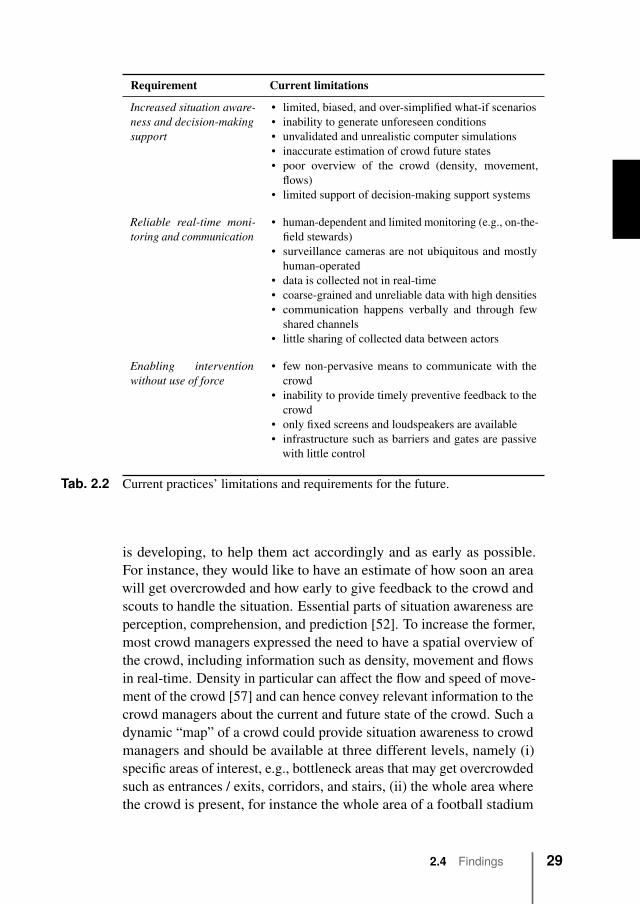
Requirement Current limitations

Increased situation aware-ness and decision-makingsupport

• limited, biased, and over-simplified what-if scenarios• inability to generate unforeseen conditions• unvalidated and unrealistic computer simulations• inaccurate estimation of crowd future states• poor overview of the crowd (density, movement,

flows)• limited support of decision-making support systems

Reliable real-time moni-toring and communication

• human-dependent and limited monitoring (e.g., on-the-field stewards)

• surveillance cameras are not ubiquitous and mostlyhuman-operated

• data is collected not in real-time• coarse-grained and unreliable data with high densities• communication happens verbally and through few

shared channels• little sharing of collected data between actors

Enabling interventionwithout use of force

• few non-pervasive means to communicate with thecrowd

• inability to provide timely preventive feedback to thecrowd

• only fixed screens and loudspeakers are available• infrastructure such as barriers and gates are passive

with little control

Tab. 2.2 Current practices’ limitations and requirements for the future.

is developing, to help them act accordingly and as early as possible.For instance, they would like to have an estimate of how soon an areawill get overcrowded and how early to give feedback to the crowd andscouts to handle the situation. Essential parts of situation awareness areperception, comprehension, and prediction [52]. To increase the former,most crowd managers expressed the need to have a spatial overview ofthe crowd, including information such as density, movement and flowsin real-time. Density in particular can affect the flow and speed of move-ment of the crowd [57] and can hence convey relevant information to thecrowd managers about the current and future state of the crowd. Such adynamic “map” of a crowd could provide situation awareness to crowdmanagers and should be available at three different levels, namely (i)specific areas of interest, e.g., bottleneck areas that may get overcrowdedsuch as entrances / exits, corridors, and stairs, (ii) the whole area wherethe crowd is present, for instance the whole area of a football stadium

2.4 Findings 29

that is used by the crowd, (iii) areas around / outside the total area ofinterest, for instance the parking areas around / leading to the footballstadium. Ideally, the map would include additional information aboutthe crowd, such as the profiles of the people, their mood, the placementof exists, stewards and other infrastructure. To increase prediction, theinformation in the map needs to include trends in crowd behavior anddynamics, and how they develop over time.

Reliable real-time monitoring and communication

Crowd managers expressed the need for reliable means to measure thestate of the crowd, that can operate particularly in critical conditions.Current “instruments” to survey large crowds are the stewards on theground inside the crowd and surveillance cameras watching over thecrowd. These approaches are limited as they may lead to personnelmissing relevant information. Feeds from the surveillance cameras aremonitored by personnel who cannot watch all screens at all times. Cur-rent automatic approaches, like computer-vision image analysis of videostreams or automatic counting from mobile phones traces, do not op-erate at high density and large-scale. Finally, crowd managers desiredto collect and integrate information currently stored in “silos” fromdifferent sources. For example, smart turnstiles and barriers are used tocollect information about the crowd for future planning. Crowd man-agers emphasized the importance of obtaining and using this informationin real-time during the event.

Similarly, crowd managers expressed need for reliable communicationwithin the team as well as with the crowd in critical conditions. Currentapproaches present limitations similar to those regarding monitoring,that is they are mostly human-dependent and manually operated, causinginformation loss or overload. For what concerns communication to thecrowd, managers stressed the need for effective means to communicatebeyond current loud-speakers and screens.

Enabling interventions without usage of force

Concerning the actions that must be taken to manage the crowds, crowdmanagers expressed the need for mechanisms to effectively control themovements of the crowd. In particular, a mechanism was sought whichwould allow the coordination of the movements of groups of people ina crowd. Conceptually, a “traffic light”, in the own terms of one of themanagers, that would control which groups of people could move, where



and when. Moreover, crowd managers expressed the need for meansto evenly distribute the crowd in a given space, e.g., a train platform ora concert area, as well as to evenly distribute the crowds in time, forexample, to prevent that large numbers of people arrive to and departfrom an event all at the same time. Solutions for queue managementin large crowds were also mentioned as important requirements, whichcould support “flexible queuing”, for example, allowing people to leaveand re-join a queue, or even “queue-less” events and help the speedingup of queues.

While some of these interventions could be implemented through newphysical and mechanical infrastructure, crowd managers acknowledgedthat in order to take actions towards the crowd, communication with thecrowd is of utmost importance. Therefore crowd managers expressedthe need to communicate well with the crowds. Mechanisms are thusneeded which can very clearly and effectively provide the crowds withinformation such as: (i) overview of the crowd situation (ii) reasons forany troubles and delays, (iii) predictions, waiting times, (iv) advices,alternatives, orders.

2.5 Recommendations: the anatomy of atechno-social system for crowd management

In this section we provide a systematic discussion on how technologymay improve the support of crowd management practices. We frameour recommendations around a techno-social system comprising of twofeedback control loops. If we consider the interaction between thecrowd management team and the crowd as a social system, then wecan define a techno-social system for crowd management as a systemwhere technology supports and augments such interaction. We envisiona system implementing data-driven practices common to other industries.Examples of such practices are (i) collection, processing and sharingof large streams of heterogeneous data coming from mobile and fixedsensors, (ii) support for analysis and sense-making of crowd data, forexample, by means of tools for exploration and visualization of largedatasets, and (iii) recommendation and implementation of interventionstrategies executed for example through actuators, such as turnstiles andbarriers, and communication. At the same time, we envision empoweredindividuals in the crowd taking autonomous decisions based on feedbackprovided by the system.

2.5 Recommendations 31

A number of different technologies and state-of-the-art techniquescan fit into such framework, and could aid tackling the limitationsand drawbacks presented in Table 2.2. In Table 2.3 we provide somehypothetical concrete examples of how the implementation of our modelwould impact on the operations outlined by the crowd managers (notehow the operations in Table 2.3 match the requirement in Table 2.2). Wego in the details in the following sections.

2.5.1 Crowd management as two feedback control loops

In a nutshell, a feedback control loop comprises three phases: (i) mea-surement of input, (ii) control of input, and (iii) actuation through feed-back. Crowd management can be seen as two of such loops. One thathappens during the event, and one that takes place between events. Look-ing at crowd management practices as feedback control loops allowsus to reason about how technology can help, in all three phases, thegroup work of crowd managers towards a more effective and data-drivenapproach. Figure 2.4 summarizes the relationship between the two loopsand their operations.

The loop within each event

The first feedback control loop takes place during the event, and com-prises all the operations to (i) collect information about the state of thecrowd, (ii) assess and predict the state of the crowd within the plannedscenarios, (iii) intervene, if necessary, to prevent uncomfortable anddangerous situations. The loops should be operated at short intervals(e.g., seconds or few minutes), to ensure real-time monitoring and quickresponse.

The measurement phase is perhaps the phase that has received mostrecent attention in the literature. Existing pervasive and ubiquitoussensing infrastructure have been proposed and investigated as a meansto measure the movement of flows of people, the areas affected byundesired crowd mood, but also the capacity of parking lots and thedevelopment of weather conditions. This infrastructure includes mobilesensors such as smart phones and RFID-enabled bracelets used as festivaltickets, as well as, for example, fixed sensors like video cameras andweather stations. However, crowd managers expressed a need for real-time measurement of crowd behavior, and a dissatisfaction with theunreliability of current solutions at high densities. Recent work on



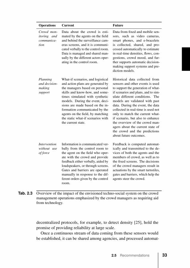
Operations Current Future

Crowd mon-itoring andcommunica-tion

Data about the crowd is esti-mated by the agents on the fieldand behind the surveillance cam-eras screens, and it is communi-cated verbally to the control room.Data is managed and shared man-ually by the different actors oper-ating in the control room.

Data from fixed and mobile sen-sors, such as video cameras,smart phones, and e-braceletsis collected, shared, and pro-cessed automatically to estimatein real-time densities, flows, con-gestions, crowd mood, and fur-ther supports automatic decision-making support systems and pre-diction models.

Planningand decision-makingsupport

What-if scenarios, and logisticaland action plans are generated bythe managers based on personalskills and know-how, and some-times simulated with syntheticmodels. During the event, deci-sions are made based on the in-formation communicated by theagents on the field, by matchingthe static what-if scenarios withthe current state.

Historical data collected fromsensors and other events is usedto support the generation of what-if scenarios and plans, and to sim-ulate different conditions. Themodels are validated with pastdata. During the event, the datacollected in real-time is used notonly to match the current what-if scenario, but also to enhancethe overview of the crowd man-agers about the current state ofthe crowd and the predictionsabout future outcomes.

Interventionwithout useof force

Information is communicated ver-bally from the control room tothe agent on the field who oper-ate with the crowd and providefeedback either verbally, aided byloudspeakers, or through screens.Gates and barriers are operatedmanually in response to the dif-ferent orders given by the controlroom.

Feedback is computed automat-ically and transmitted to the de-vices of both the agents and themembers of crowd, as well as tothe fixed screens. The decisionsof the crowd managers result inactuations by the smart turnstiles,gates and barriers, which help theagents steer the crowd.

Tab. 2.3 Overview of the impact of the envisioned techno-social system on the crowdmanagement operations emphasized by the crowd managers as requiring aidfrom technology.

decentralized protocols, for example, to detect density [25], hold thepromise of providing reliability at large scale.

Once a continuous stream of data coming from these sensors wouldbe established, it can be shared among agencies, and processed automat-


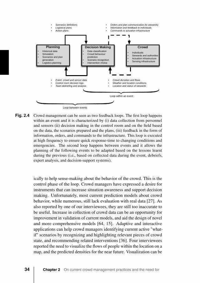
Planning Decision Making Crowd

Loop between events

Loop within an event

• Historical data• Simulation• Scenarios and plan

generation• Logistics planning

• Data classification• Crowd behaviour

prediction• Scenario recognition• Intervention choice

• Individuals• Stewards and authorities• Actuation infrastructure• Sensing infrastructure

• Orders and plan communication (to stewards)• Information and feedback to individuals• Commands to actuation infrastructure

• Crowd densities and flows• Weather and location conditions• Location and status of stewards

• Scenarios definitions• Logistical plans• Action plans

• Event, crowd and sensor data• Control room decision logs• Team debriefing and analysis

Fig. 2.4 Crowd management can be seen as two feedback loops. The first loop happenswithin an event and it is characterized by (i) data collection from personneland sensors (ii) decision making in the control room and on the field basedon the data, the scenarios prepared and the plans, (iii) feedback in the form ofinformation, orders, and commands to the infrastructure. This loop is executedat high frequency to ensure quick response-time to changing conditions andemergencies. The second loop happens between events and it allows theplanning of the following events to be adapted based on the lessons learntduring the previous (i.e., based on collected data during the event, debriefs,expert analysis, and decision-support systems).

ically to help sense-making about the behavior of the crowd. This is thecontrol phase of the loop. Crowd managers have expressed a desire forinstruments that can increase situation awareness and support decisionmaking. Unfortunately, most current prediction models about crowdbehavior, while numerous, still lack evaluation with real data [27]. Asalso reported by one of our interviewees, they are still too inaccurate tobe useful. Increase in collection of crowd data can be an opportunity forimprovement in validation of current models, and aid the design of noveland more comprehensive models [64, 15]. Adaptive and interactiveapplications can help crowd managers identifying current active "what-if" scenarios by recognizing and highlighting relevant pieces of crowdstate, and recommending related interventions [36]. Four intervieweesreported the need to visualize the flows of people within the location on amap, and the predicted densities for the near future. Visualization can be



a powerful tool to facilitate computer-supported cooperative work [75].Current work on visualization of mobility traces within urban areas andlarge scale festivals provide examples of such interfaces [101, 152].

Regarding the feedback phase, again smart phones and other wearabledevices are an opportunity for crowd managers to communicate withcrowd members, and platforms to support autonomous decisions by theindividuals in the crowd. For example, apps running on smart phonescan allow fine-grained location-aware communication targeted to spe-cific zones of the event location with personalized information [155].While current music festival apps allow to share and visualize the loca-tion of friends on a map, they do not display, for example, the flows ofpeople between stages, or the densities around the different spots. Suchinformation, automatically provided by the system, could allow individ-uals to make informed decision, and avoid unpleasant situations [19].With respect to fixed infrastructure, barriers are also opportunities tocommunicate information about the state of the crowd, for example,through a displays showing densities at the front of a queue or near anexit, or by indicating alternative routes through lights.

The loop between events

The second feedback control loop consists of the process of crowdmanagement itself, and includes (i) debriefing outcomes of a previousevent, (ii) analyzing possible flaws in the plan or in the decision makingprocess, and (iii) updating of the planning processes to accommodatenew lessons.

The utility of the information collected during an event does not finishat the end of the event. The databases of sensed data, together withthe log of decisions made by the management team during the event,provide a solid base for a systematic reasoning about the outcome ofthe event [89]. Interviewees underlined the generation of the what-ifscenarios as being at risk of bias, lack of coverage and depth. A moredata-driven approach can reduce errors and bias, as well as allow expertsto recognize new scenario that happened during th event. Scenarios canbe recommended to the crowd managers based on the data collected overtime, during previous events. Moreover, such scenarios can be automati-cally characterized by estimates based on historical data. Also, data canfacilitate the reviewing procedures at the end of the event [65]. Finally,sensed data can be fed into crowd behavior simulators, to overcome theaforementioned limitations related to absence of rich scenarios and vali-dation [64, 59], or fed into computational models to support operational


research techniques for task force deployment [47]. The result is a liveprocess, where data-driven approaches support collaboration within thecrowd management team from the phase of planning to the phase ofimplementation, during and between events.

2.5.2 ImplicationsIn this section we discuss implications and constraints that need to beconsidered when introducing more technology within such a techno-social system.

Keeping the human in the loop

While we advocate a bigger role of technology in crowd management,we emphasize that such transition shall happen with the human, bothas a member of the crowd management team and of the crowd, in thecenter. When designing crowd applications, one should take into accountexplicit and implicit motivational factors. For instance, users in thecrowd may require incentives to share their data and, for example, utilizean energy-consuming application on their phone. Providing a platformto help locate friends could be an example of an incentive to sharewith the system current locations and social ties. Moreover, individualshave different psychological needs when it comes to well-being [91].Crowd members seek for fulfilling higher level of psychological needs,i.e., staying autonomous, connected, competent and respected in normalcrowd conditions, while their focus will immediately change to low levelneeds, i.e., safety and security issues, when unexpected things happen.

For what concerns crowd managers, it is important to support theirplanning and collaborative decision-making, in particular in emergencysituations [77]. Interviewees pointed out that current technologicalsolutions often lack comprehensiveness or accuracy, which resultedin rejection of the system. Perceived usefulness of an instrument isknown to be strongly influencing the intentions of the user, even morethan perceived ease [39]. Importantly, the goal of decision-supportsystem should be to aid the expert decision of a crowd manager, and notsubstitute it [122].

Guaranteeing privacy to the crowd

While not directly mentioned by the interviewees, ensuring privacy andtrust are critical adoption barriers of such a system. For example, detec-tion of flows and bottlenecks as well as mood, require constant probing



for sensitive information such as location and emotions. Moreover, pri-vacy is user specific, that is each individual has a different perceptionof privacy. Various techniques have been proposed to solve the issue ofprivacy in sensing, and they include anonymization [135], cryptographictechniques [160, 54], and data obfuscation [5, 61]. Crowd data, in par-ticular with respect to crowd dynamics, lends itself to these techniques.For example, the characterization of pedestrian flows and their volumes,does not require knowledge about the identity of the comprising users.

Minimizing the need for new infrastructure

Introducing technology can often imply new and expensive investments.Two distinctions are necessary in this case. First, there are gatheringsthat take place in fixed locations, designed for the purpose of hostingcrowds. Examples are train stations, music halls, stadiums, and theaters.These locations already employ substantial infrastructure, starting frombarriers, video cameras, turnstiles, sometimes Bluetooth and Wifi scan-ners. In these scenarios, the interviewees reported being open to theinstallation of new infrastructure, given a reliable functioning in criticalconditions.

Second, there are events that take place in locations that are not de-signed to host large crowds. For example, periodic parades and celebra-tions taking place in city centers and neighborhoods. In these occasions,it is difficult and expensive to temporarily deploy new infrastructurespervasively across town. As reported by the interviewees, smart phonesare widely adopted and minimize the need for additional infrastructure.Moreover, event planners often cooperate with telecom companies toobtain cellular data about densities. Finally, additional cellular towerscan sometimes be installed to alleviate the problems of congestion.

2.6 DiscussionWe interviewed 10 crowd managers to gain an understanding of thecurrent role of technology in their current practices, including limitationsand requirements. We have formulated our recommendations within atechno-social system framework. Despite the fact that the 10 volunteersagreed on many of the fundamental definitions about their practicesand needs, regardless of their diverse domains of work, it is likely thatour results are influenced by different biases, for example, cultural,organizational, and geographical, as all the managers operate in TheNetherlands. To be able to generalize the results of the interviews

2.6 Discussion 37

more work needs to be done in different geographical, cultural andeconomical contexts. Nonetheless, the consistency of our results withthe other work [29, 65, 18] suggests that our results can be generalizableat least to similar contexts to those in the Netherlands.

While the volunteers are indeed experts with decades of experience,we should not treat the data completely as “ground truth”. To vali-date some of the statements and assumptions, further on-ground andobservational work should complement the insights extracted from theinterviews. We suggest this work to be conducted both in the controlroom and on the field, during the different phases of the planning andimplementation of an event.

It is unclear whether many of the technological problems and limi-tations we described in this chapter are specific to crowd management,and how much of the related research should be adapted to in the contextof crowd management specifically. For example, radio-based communi-cation is known to operate poorly at high densities and hence it does notrepresent a crowd-specific problem. Yet, crowds are not characterizedsolely by high densities but also by movement patterns that are innateand hence exploited, for example, by so-called epidemic protocols usedby wireless sensors to disseminate data and communicate at large. At thesame time, the bodies of individuals influence communication in a muchdifferent way than metallic objects as, for example, cars, making someof the related work on transportation systems not directly applicable tocrowds.

The vast majority of existing literature on crowd and pedestrian behav-ior focuses on modeling and predicting behavior. More recent work hasfocused on how to devise sensing infrastructure to collect real-time dataabout the behavior of a crowd, and support sense-making. Less attentionhas been dedicated to how to support crowd management specific deci-sion making and even less to how to intervene and steer crowd behaviorto ensure the safety of the individuals. Tackling these challenges requiresmulti-disciplinary work that comprises investigating how to influencethe behavior of a crowd, how to choose the right action to obtain acertain reaction from the crowd, what information to communicate tothe crowd and with which medium and feedback. Answers to thesequestions are far from trivial and, to this date, mostly unknown.



2.7 ConclusionsWe have presented crowd management as a set of collaborative practices.The successful management of an event depends on the cooperation andcommunication between these actors, and the crowd. Our findings showthat crowd managers do already look at technology to solve some oftheir problems, and see it as an opportunity for future developments.As technology plays a bigger role in crowd management, a number oftechnical and technological challenges need to be tackled, from differentfields and practices. We have addressed these challenges within theframework of a techno-social system. This work shows that there isspace for more support from technology at different stages of the plan-ning and implementation of an event, and it motivates and suggests newdirections for research to support the safe management of crowds.

2.7 Conclusions 39

3Crowd textures as proximitygraphs

„Perfection is reached not when there isnothing left to add, but when there isnothing left to take away.

— Antoine de Saint Exupéry

3.1 IntroductionIn the previous chapter we have seen that crowd managers are lackingproper support from technology when it comes to situation awareness,prediction, and intervention. The core behaviors pointed out by theinterviewees are behaviors with a strong spatio-temporal nature, inparticular so-called crowd dynamics. In this dissertation, I argue thatrelative-proximity information can be leveraged to help researchersand practitioners understanding, among other social behaviors, crowddynamics, towards filling the gaps identified by the crowd managers.

The term “crowd dynamics” is used to refer to patterns of crowdmovement, and more precisely to “the coordinated movement of a largenumber of individuals to which a semantically relevant meaning can beattributed, depending on the respective application” [120]. Examplesinclude a queue of people, the formation of uni-directional “lanes” inbi-directional pedestrian flows, the intersection of these lanes, or agroup of people at a specific location. We use the phrase texture of acrowd to express the spatio-temporal relationships resulting from theinterdependencies in the social fabric of a group of people. At this stagewe may not yet fully understand what potential insights can be derivedfrom crowd textures, but in any case it enables the study of emergent

The contents of this chapter have been originally published in “Crowd textures asproximity graphs” C. Martella, A. van Halteren, M. van Steen, J. Li, C. Conrado -IEEE Communications Magazine 2014, and have been slightly modified to improvereadability.

41

spatio-temporal and social behavior of people in a crowd. For example,it allows one to question to what extent a group is dispersed in a crowd.

Discovering and investigating the texture of a crowd is at the heartof research in crowd management. As a prerequisite, it is essential toadequately represent texture. A common approach is to simply placecameras and collect their images and videos. There are a few drawbacks:the computational cost of video analysis limits the scale at which ex-periments can be run, cameras can be affected by complications suchas occlusion and incomplete coverage, and privacy issues can emergewhen the footage is recorded from real-world events.

As an alternative, on-body sensors can be used. Such sensors cancollect rich information about the individual behavior of each subject.We believe a better understanding of crowd dynamics can be achieved bysensing from within the crowd instead of from an external observationpoint, as the sensing is based directly on the crowd: the individualsforming the crowd. An example of this approach can be found in [120]where accelerometers are used to recognize groups of people walkingtogether.

A crowd is more than just a sum of individuals and collective behaviorresults from a continuous interaction and mutual influence between eachindividual and those nearby. The literature presents a vast number ofexamples of such behaviors as exhibited by animals such as swarmsof insects, flocks of birds and schools of fish, and there is evidence ofherding behavior also in humans [49]. Such networks of influence arefundamental for the emergence of collective behavior and are based bothon the spatial relationship between the individuals as well as their socialrelationships.

In this chapter, we address the representation of the texture of a crowdthrough a (dynamic) proximity graph1. The proximity graph provides acomputational representation of a crowd over time, it allows the analysisof the crowd texture it represents, and it provides a way to compute theeffects of interventions into the crowd.

Modeling relationships between individuals through a graph is notnew. Social graphs represent social relationships between individualsthrough edges. Also, on-body sensors have been used to actually mea-sure social graphs [32, 74]. Finally, since a few years various groupshave been dedicated to gathering data on the mobility of people.

1Our definition of proximity graph should not be confused with that of a RelativeNeighborhood Graph, although the two share some of their properties.

42 Chapter 3 Crowd textures as proximity graphs

However, using a spatio-temporal graph to represent the texture of acrowd has not been done before, and we are not aware of any attempts todo so at the scale of (tens of) thousands of people. Besides its intendedscale, the novelty of the proposed approach lays in the content of theproximity graph and the semantic interpretation of an edge. At a specificmoment in time, an edge merely represents that two individuals wereclose to each other. Measurements over prolonged periods will revealsocial groups (as we will discuss in this chapter), spatial structures (likelanes, clogging, and so on), but also the changes in the texture that resultfrom targeted interventions (like displaying announcements on a largepublic display). The main contribution of this chapter is introducingthe concept of crowd textures and their representation with proximitygraphs.

The remainder of this chapter is organized as follows. We connectthe local spatio-temporal nature of crowds and crowd dynamics to theconcept of crowd texture. We then introduce the proximity graph asa representation of crowd textures, along with analytic examples. Wedescribe a system architecture for an instrument to extract a series ofproximity graphs from a crowd, analyze it, and communicate feedback tothe crowd. We present an analysis of the proximity graphs we collectedduring a real-world experiment through a wearable device. We concludeby discussing possible extensions to the presented work.

3.2 Crowds and crowd dynamics

A generally accepted definition of a crowd is that it is a sizable numberof individuals gathered together at a specific location with a sufficientdensity distribution, for a measurable amount of time and for a specificpurpose. Moreover, the individuals in a crowd generally act in a coher-ent manner, sharing a social identity and common goals, interests andbehavior, in spite of coming together in a typically unfamiliar situation.

Crowd behavioral patterns emerge from individual human interactions,which typically have a strong local character: individuals in a crowdinfluence one another, and this influence is stronger between nearbyindividuals. In fact, several models of crowd dynamics - which giverise to large-scale emergent behavioral patterns - do take into accountlocal interactions between individuals, as well as the related measures ofcrowd density. For example, the social force model and its extension forpanicking pedestrians [66] considers physical forces between individuals(as well as forces between individuals and the environment). The forces

3.2 Crowds and crowd dynamics 43

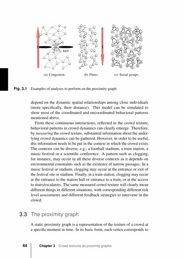
(a) Congestion. (b) Flows. (c) Social groups.

Fig. 3.1 Examples of analyses to perform on the proximity graph.

depend on the dynamic spatial relationships among close individuals(more specifically, their distance). This model can be simulated toshow most of the coordinated and uncoordinated behavioral patternsmentioned above.

From these continuous interactions, reflected in the crowd texture,behavioral patterns in crowd dynamics can clearly emerge. Therefore,by measuring the crowd texture, substantial information about the under-lying crowd dynamics can be gathered. However, in order to be useful,this information needs to be put in the context in which the crowd exists.The contexts can be diverse, e.g., a football stadium, a train station, amusic festival or a scientific conference. A pattern such as clogging,for instance, may occur in all these diverse contexts as it depends onenvironmental constraints such as the existence of narrow passages. In amusic festival or stadium, clogging may occur at the entrance or exit ofthe festival site or stadium. Finally, in a train station, clogging may occurat the entrance to the station hall or entrance to a train, or at the accessto stairs/escalators. The same measured crowd texture will clearly meandifferent things in different situations, with corresponding different risklevel assessments and different feedback strategies to intervene in thecrowd.

3.3 The proximity graphA static proximity graph is a representation of the texture of a crowd ata specific moment in time. In its basic form, each vertex corresponds to


an individual. Two vertices are joined by an edge if the two individualsthey stand for happened to be in physical proximity, within a chosendistance. Each edge represents only the Boolean relationship withoutcapturing the actual distance. Time is generally discretized into smallslots. If and only if two individuals were detected to be in each other’sproximity during a time slot, their associated vertices will be joinedby an edge for that slot. A proximity graph is therefore dynamic; wespeak of a proximity graph at time t as a (proximity graph) snapshot att. Note that a proximity graph is naturally represented by a time seriesof proximity-graph snapshots. Although a proximity graph containsspatial information, it does not rely on absolute positioning data. It isthe global representation of the texture of a crowd constructed from thelocal perspective of individuals within that crowd.

A proximity graph incorporates information to support the model-ing of crowd dynamics where the individual behavior is defined onlyon relative neighborhood information. Basic models of flocking be-havior are of this kind, as they are controlled by the following simplerules [119]. (1) Separation: avoid crowding neighbors (short rangerepulsion), (2) Alignment: steer towards average heading of neighbors,(3) Cohesion: steer towards average position of neighbors (short rangeattraction) . Each of the three rules can be applied by a member of thecrowd based only on local information, namely its neighbors’ states,and no global view or absolute spatial reference points are necessary.This type of modeling has been successfully applied to human herdingbehavior as well [49]. The above set of rules has been extended indifferent ways since its introduction to incorporate emotions, leadershipetc.

3.3.1 Analyzing the proximity graphs

We now introduce a few examples of categories of analyses that couldbe performed on proximity graphs, which correspond to the contextsmentioned in the previous section.

Figure 3.1(a) presents a scenario where a crowd is exiting a stadium.As each individual approaches the exit, the local density increases giventhe physical bottleneck imposed by the gate. In the proximity graph, thelocal density is represented for each vertex by its degree, the number ofincident edges (depicted in the figure for a particular vertex with thickerlines). Recognizing a congestion requires measuring the gradient of theaverage density of a crowd as it approaches the exit.

3.3 The proximity graph 45

Figure 3.1(b) presents a scenario at a train station where a pedestrianflow is forming on a platform. There are two groups of individuals: onthe left there is a stationary group waiting for a train, on the right thereis another group that has just stepped out of another train and is headingtowards the exit. The detection of the pedestrian groups is based on thetransience of edges. In a time interval, the transience of edges, and theirrepetition, determines the degree to which neighborhoods remain thesame. Intra-group edges present a relative stability. Instead, inter-groupedges, depicted in red in the figure, are characterized by a short-livingnature. By filtering out these edges, it is possible to detect the twoconnected components representing the two groups.

Figure 3.1(c) presents a scenario at a music festival. This type of eventis usually attended by groups of socially related individuals that tend tostick together during its course. Nonetheless, groups might occasionallysplit e.g., to reach the bar, the rest room, or due to the density in frontof the stage. In the figure, we picture a moment where a crowd standsin front of a stage. The edges represent the current proximity betweenthe individuals, and the thickness represents the accumulated time spentclose to each other over the whole period. Edges representing pastproximity have not been drawn. In fact, they are not valid to describethe current crowd texture, but are used to compute the accumulated time.The detection of social groups requires preserving only the edges thatpresent a long-lasting time interval when compared to the others. Eachvertex is annotated with a group label it has been assigned to. Note thatvertices that are far apart can still belong to the same group as some ofits members might have currently and temporarily split.

3.3.2 The awareness of the contextUp to this point, we have considered vertices corresponding only toindividuals. However, the proximity graph can be extended to representother types of objects as well, e.g., a door, an ATM, or a food stand. Thistype of extension allows for a semantic and contextual interpretation ofthe observed behavior. In fact, different interpretations can be applied tothe same crowd texture, depending on the context where the observationtook place. Figure 3.2 presents an example of how the same proximitygraph can be interpreted differently. Knowing it was collected in frontof an ATM, the left-most graph can be interpreted as a queue. Instead,the same graph can represent an orchestra, knowing that the contextwas a stage (in this case the right-most vertex in the graph correspondsto the conductor while the other vertices correspond to the musicians).


Fig. 3.2 Example of the dependency of the proximity graph on contextual information.

Location awareness allows for the disambiguation of the meaning aproximity graph can assume.

The concept of awareness can be generalized through annotations.An annotation to a vertex is a key-value pair that describes a specificproperty of the object represented by that vertex, e.g., gender, age, exitnumber, gate capacity, GPS coordinate, staff role, etc. Annotations con-tribute to awareness as they allow to picture more precisely the observedtexture and support informed decision-making. For example, throughan annotated graph it is possible to recognize at what specific exit acongestion has formed, if children are involved, or whether stewardsare already around the area for support. Also, static vertices with GPScoordinates annotations can act as absolute positioning reference pointswhen necessary.

A consequence of the relative nature of the proximity graph is thatmovement cannot be attributed to vertices. An edge “breaks” whenat least one of the two individuals involved in the relationship movesaway. As the result of these actions is the same, determining whichone occurred is not possible. Going back to the platform example inFigure 3.1(b), recognizing the short-living edges, depicted in red, allowsfor the detection of relative movement between the two groups. Again,it is not possible to determine for each group whether it is moving ornot. Extending the graph with static vertices spread along the platformprovides a solution to the problem. In fact, the vertices belonging to themoving groups would create short-living edges with these static verticesallowing inference of movement.

The temporal information encoded in the proximity graph allows formore than the description of crowd dynamics. As proximity can bea by-product of social interaction, socially related individuals tend to

3.3 The proximity graph 47

spend more time close to each other than strangers. This principle is atthe basis of the example depicted in Figure 3.1(c). For example, in [32]the authors were able to analyze the social ties within organizations bylooking at low-frequency proximity information. In general, knowinghow much time two or more individuals have spent close to each other,with possible addition of contextual information about location, enablesthe inference of the type of social relation incurring between them.

Temporal information also enables the inference of consequentiality.Imagine the festival scenario depicted in Figure 3.1(c). Suppose weobserve individual A conversing first with B and later with C. If, lateron, we would note A, B and C conversing together, we could imaginethat B and C were introduced by A. In the same way, we could predictthat an individual who was observed in proximity to a counter, wheretickets for drinks are sold, will eventually show up at the bar. Similarly,the temporal dimension of face-to-face interactions has also been inves-tigated to study the spreading patterns of epidemic diseases in differenttypes of social events, e.g., a conference or a museum [74].

3.4 An instrumentWe identify the following requirements for an instrument to measureand analyze the proximity graphs presented thus far. (1) It is composedof a device that is wearable by an individual, and (2) that is detectable,within a chosen distance range, to measure proximity. (3) The infor-mation measured by the devices is extracted and collected through aninfrastructure. (4) The collected proximity graph is analyzed by a pro-cessing system looking for patterns, and (5) feedback is transmitted fromthe system to the individuals.

One notable way to implement our sensing device is an applicationrunning on a mobile phone. Mobile phones are widely diffused acrossthe population, and already ship with both high computing power, e.g.,dual-core processors, and a broad range of sensors, e.g., accelerometers,microphones, cameras etc. On the other hand, with the decrease inprice and size of wearable technology, another way of implementingour device is through a smart chip-card, such as those currently usedfor public transport tickets or for badges on the working places (thesame technology can be easily integrated into a festival bracelet as well).Figure 3.5(a) shows the device we currently use for our experimentswith the proximity graph. We return to its description shortly.


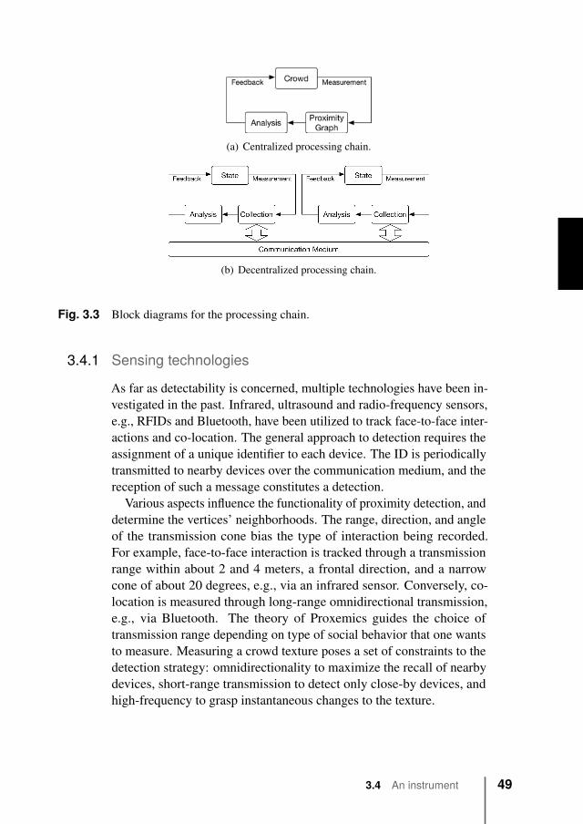
(a) Centralized processing chain.

(b) Decentralized processing chain.

Fig. 3.3 Block diagrams for the processing chain.

3.4.1 Sensing technologies

As far as detectability is concerned, multiple technologies have been in-vestigated in the past. Infrared, ultrasound and radio-frequency sensors,e.g., RFIDs and Bluetooth, have been utilized to track face-to-face inter-actions and co-location. The general approach to detection requires theassignment of a unique identifier to each device. The ID is periodicallytransmitted to nearby devices over the communication medium, and thereception of such a message constitutes a detection.

Various aspects influence the functionality of proximity detection, anddetermine the vertices’ neighborhoods. The range, direction, and angleof the transmission cone bias the type of interaction being recorded.For example, face-to-face interaction is tracked through a transmissionrange within about 2 and 4 meters, a frontal direction, and a narrowcone of about 20 degrees, e.g., via an infrared sensor. Conversely, co-location is measured through long-range omnidirectional transmission,e.g., via Bluetooth. The theory of Proxemics guides the choice oftransmission range depending on type of social behavior that one wantsto measure. Measuring a crowd texture poses a set of constraints to thedetection strategy: omnidirectionality to maximize the recall of nearbydevices, short-range transmission to detect only close-by devices, andhigh-frequency to grasp instantaneous changes to the texture.

3.4 An instrument 49

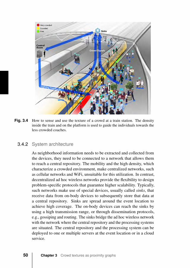
Fig. 3.4 How to sense and use the texture of a crowd at a train station. The densityinside the train and on the platform is used to guide the individuals towards theless crowded coaches.

3.4.2 System architecture

As neighborhood information needs to be extracted and collected fromthe devices, they need to be connected to a network that allows themto reach a central repository. The mobility and the high density, whichcharacterize a crowded environment, make centralized networks, suchas cellular networks and WiFi, unsuitable for this utilization. In contrast,decentralized ad hoc wireless networks provide the flexibility to designproblem-specific protocols that guarantee higher scalability. Typically,such networks make use of special devices, usually called sinks, thatreceive data from on-body devices to subsequently store that data ata central repository. Sinks are spread around the event location toachieve high coverage. The on-body devices can reach the sinks byusing a high transmission range, or through dissemination protocols,e.g., gossiping and routing. The sinks bridge the ad hoc wireless networkwith the network where the central repository and the processing systemsare situated. The central repository and the processing system can bedeployed to one or multiple servers at the event location or in a cloudservice.


We connect the devices through an ad hoc wireless network, as itmatches the given constraints while enabling both the transmissionof detection messages and the exchange of information between thedevices. Also, it allows for the communication with the external networkfor processing and feedback.

While data streams from the devices to the central repository, theglobal view of the proximity graph gets constantly updated. Periodi-cally, the processing system analyses the proximity graph, examiningthe crowd texture for known patterns. Recognition of crowd dynamicsis a classification problem that requires statistical analysis of the metricsof the graph, either at vertex, group, or global level. The temporal in-formation in the proximity graph is exploited by analyzing snapshots,defined by time intervals whose duration depends on the analysis beingperformed. Graph algorithms are potentially computationally expensive,introducing additional latency between the measurement and the recog-nition of patterns. This requires a system with sufficient computationalpower to analyze a proximity graph within the required time constraints.

Once the information is extracted from the proximity graph, it canbe presented for feedback. The feedback can be sent to the crowdmanagers or directly to the crowd, either through the devices or throughfixed infrastructure, e.g., screens, speakers, etc. While feedback canreach the control room and the infrastructure over the reliable network,devices can be reached via the ad hoc wireless network. In the same wayinformation is extracted and collected from the devices, disseminationprotocols allow feedback to reach specific individuals, groups or thewhole crowd. The intervention strategy defines the information, thedestinations, and the techniques used to give feedback to the crowd.

3.4.3 A processing chainWe present now a processing chain that incorporates all the compo-nents presented above into a loop. The processing loop is presented inFigure 3.3(a). Each individual wears a device with a proximity sensorcapable of detecting the other devices within a chosen distance range.The devices share a communication medium that enables transfer ofinformation. The loop starts with the measurement of the individual’sneighborhood through the device’s sensor. Once the neighborhoods aremeasured, the next step consists in the collection of the neighborhoodsfrom the devices to a central repository, to compose the global view ofthe proximity graph. Afterwards, the proximity graph can be analyzedby a processing system to recognize crowd dynamics. Possibly, feedback

3.4 An instrument 51

is computed, and sent to the managers or to the crowd. At this point, thenew state of the crowd can be measured and the loop can start again.

Figure 3.4 shows a possible future instantiation. People at a trainstation are assumed to have proximity sensors, for example, embeddedinto their smart phones, allowing for the detection of a proximity graph.The analysis of the situation in the train and on the platform may beused to subsequently inform people where to board, or to leave the train.

Note that centralization is not strictly necessary to the instrument. Asindividual behavior depends on local context represented by the indi-viduals and the objects in close proximity, the analysis algorithm canoften be expressed based on a vertex-centric local view of the graph.Following this approach, nearby devices can exchange their neighbor-hoods right after the measurement step, and analyze their local view ofthe graph autonomously, without relying on a global view of the graphcontained in the central repository. This autonomy decreases the intervalbetween the moment the state of the crowd is measured, and the momentfeedback can be generated. This alternative is presented in Figure 3.3(b).However, a third possibility is available: a hybrid system where thedevices locally aggregate and process proximity information, and onlythese aggregated views are later collected and processed centrally. Thislatter approach provides both decreased latency in feedback generationand central monitoring of the crowd. Moreover, it minimizes the over-head of data extraction from the devices, as only aggregated informationis transmitted.

3.5 Real-world experiment

To give a flavor of what can be achieved following our approach, inthis section we describe an example application based on a real-worldexperiment we conducted at an ICT conference. The conference wasdivided into 7 tracks, each focusing on a specific ICT topic, such asHigh-Performance Computing, Software Engineering, Security, etc. Ofthe 250 attending individuals, 139 were wearing one of our devices as aname tag throughout the whole day. We asked each of the participantsfor their main track of interest, as a hint to community membership(note that the groups were not balanced, as for example one had onlyfour individuals participating in the experiment). Table 3.1 shows thedistribution of the participants across the tracks. The device, depictedin Figure 3.5(a), has an Atmel ATXMega128 CPU with 8k of RAM,128k of flash memory, and a Nordic nRF24L01+ wireless radio. To


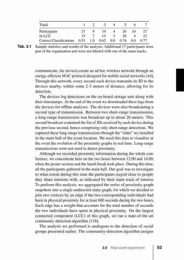
Track 1 2 3 4 5 6 7

Participants 27 9 19 4 26 10 27In LCC 15 7 13 3 20 4 22Correct Classifications 0.53 1.0 0.62 0.0 0.74 0.0 0.77

Tab. 3.1 Sample statistics and results of the analysis. Additional 17 participants werepart of the organization and were not labeled with one of the main tracks.

communicate, the devices create an ad hoc wireless network through anenergy-efficient MAC protocol designed for mobile social networks [44].Through this network, every second each device transmits its ID to thedevices nearby, within some 2-3 meters of distance, allowing for itsdetection.

The devices log detections on the on-board storage unit along withtheir timestamps. At the end of the event we downloaded these logs fromthe devices for offline analyses. The devices were also broadcasting asecond type of transmission. Between two short-range transmissions,a long-range transmission was broadcast up to about 20 meters. Thissecond broadcast contained the list of IDs received by each device duringthe previous second, hence comprising only short-range detections. Wecaptured these long-range transmissions through the “sinks” we installedin the main hall of the event location. We used this data to visualize atthe event the evolution of the proximity graphs in real time. Long-rangetransmissions were not used to detect proximity.

Although we recorded proximity information during the whole con-ference, we concentrate here on the two hours between 12:00 and 14:00,when the poster session and the lunch break took place. During this time,all the participants gathered in the main hall. Our goal was to investigateto what extent during this time the participants stayed close to peoplethey share interests with, as indicated by their main track of interest.To perform this analysis, we aggregated the series of proximity-graphsnapshots into a single undirected static graph, for which we decided tojoin two vertices by an edge if the two corresponding individuals hadbeen in physical proximity for at least 600 seconds during the two hours.Each edge has a weight that accounts for the total number of secondsthe two individuals have spent in physical proximity. On the largestconnected component (LCC) of this graph, we ran a state-of-the-artcommunity-detection algorithm [116].

The analysis we performed is analogous to the detection of socialgroups presented earlier. The community-detection algorithm assigns

3.5 Real-world experiment 53

vertices to communities trying to maximize modularity. Graphs withhigh modularity tend to have dense connections between vertices withincommunities and sparse connections between vertices across differentcommunities. Intuitively, it groups together vertices that are intercon-nected and have spent long time together. Figure 3.5(b) shows the resultsof the analysis. Vertices are colored according to the community theyhave been assigned to by the algorithm, and labeled according to themain topic of interest. The clustering tends to assign vertices with thesame label to the same community, supporting our hypothesis and show-ing the validity of the data extracted through the instrument. Note thatthe algorithm does not make use of the noted information about interests,but only of the topology of the graph. One should not consider themain track of interest as ground truth. In fact, many of the individualsindicated their interest as one of out of more possible ones. Moreover,as the participants came from a number of universities and departments,they tended to socialize also according to different criteria, for example,with people with whom they shared affiliation. Finally, the nature ofposter sessions and banquets stimulate people to spend time in proximityto people belonging to different communities. We leave a deeper andmore sophisticated analysis of the experiment for future work.

The unreliability of the wireless communication and of the devicescauses mis-detections, meaning that detections are missed or erroneouslyadded. Typical examples of these causes are “collisions,” interferencesof other sources of radio-frequencies (such as WiFi spots), the shieldingof the human body, data corruption due to faults in the device, etc.For this reason, to extract the proximity graphs used in our analysiswe pre-processed the logs with a density-based clustering algorithm.The algorithms exploits the “bursty” nature of the collected data toreconstruct part of the missed detections and filter out noise. Our resultsshow that this filtering phase greatly increases the sensitivity of theinstrument [98] (see Chapter 4).

3.6 Discussion

The local nature of individual behavior in crowds also affects the analysisof crowd dynamics through other modalities. In [120], the authorspropose a processing chain for the recognition of crowd behavior frommobile sensors with pattern analysis and graph clustering. Subjectswear on-body sensors, and move collectively. Activity patterns arethen extracted from the sensors for individual behavior recognition, e.g.,


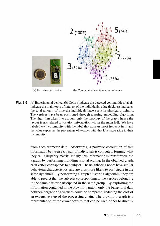
(a) Experimental device. (b) Community detection at a conference.

Fig. 3.5 (a) Experimental device. (b) Colors indicate the detected communities, labelsindicate the main topic of interest of the individuals, edge thickness indicatesthe total amount of time the individuals have spent in physical proximity.The vertices have been positioned through a spring-embedding algorithm.The algorithm takes into account only the topology of the graph, hence thelayout is not related to location information within the main hall. We havelabeled each community with the label that appears most frequent in it, andthe value expresses the percentage of vertices with that label appearing in theircommunity.

from accelerometer data. Afterwards, a pairwise correlation of thisinformation between each pair of individuals is computed, forming whatthey call a disparity matrix. Finally, this information is transformed intoa graph by performing multidimensional scaling. In the obtained graph,each vertex corresponds to a subject. The neighboring nodes have similarbehavioral characteristics, and are thus more likely to participate in thesame dynamics. By performing a graph clustering algorithm, they areable to predict that the subjects corresponding to the vertices belongingto the same cluster participated in the same group. By exploiting theinformation contained in the proximity graph, only the behavioral databetween neighboring vertices could be compared, reducing the cost ofan expensive step of the processing chain. The proximity graph is arepresentation of the crowd texture that can be used either to directly

3.6 Discussion 55

recognize crowd dynamics, or to support recognition through othermodalities.

The mutual influence between individuals is an interesting aspectof social behavior, as it can be used to guide a crowd by targeting asubset of the individuals through feedback information about the currentstate. Although during the last few years, we are starting to betterunderstand crowd dynamics, less is known about how to influence acrowd. The proximity graph is a representation of a crowd and it allowsto compute interventions towards a desired behavior. Consider thefollowing (admittedly still speculative) examples of simple interventionson crowds as presented previously in their scenarios.

The example in Figure 3.1(a) could represent a bottleneck at theentrance of a stadium. This is a typical situation where people getpushed, and in the most dramatic conditions also walked over. Thisbehavior often finds its origins in the absence of information. Theindividuals at the back of the crowd cannot see the high density at theentrance, or the presence of a congestion, and may start to push. Ascreen on top of the gate, visible for all the individuals, could depictwith colors the density in the front.

The example in Figure 3.1(b) could represent a platform in a trainstation. A common situation in such a scenario is that people getting outof the train tend to head towards the closest exit. Uneven usage of exitscould be avoided by feeding back information about less crowded exits.

Finally, the example in Figure 3.1(c) could represent groups of visitorsto a festival. Such events are usually visited by groups of friends. It iscommon that people lose contact with some members of their group.Once the groups are detected, each member of the same group can beguided towards the same exit, so that they can find each other there.

These are just a few examples of the many possibilities that emergeonce the texture of a crowd is captured in a proximity graph. Ourapproach has great potential to accelerate the emerging field of Com-putational Social Science. In particular, the capability of sensing thecrowd from within, without any requirement for location information orcentralization, in respect of the privacy of the individuals in the crowd.Moreover, it allows to compute timely insights about the state of thecrowd, and communicate feedback to ensure safety and comfort.


3.7 ConclusionsWe have presented the concept of a crowd texture as the set of spatio-temporal relationships between the crowd members that results fromtheir behavior. We have presented a series of proximity graphs asa representation of such crowd textures. We have characterized theproperties and limitations of the model, together with its extension toperson-to-object relationships, and additional information about thecontext in which the crowd is embedded.

A number of approaches were suggested to identify a number ofselected crowd dynamics, as algorithms that mine a series of proximitygraphs. We have described a distributed architecture of a system tomeasure, collect, and store the series of proximity graph, as well asprocess the graphs to identify crowd behavior. Finally, we have presenteda real-world use case where we have applied a graph-clustering algorithmto a series of proximity graphs collected during an ICT conference, todemonstrate that social groups in the crowd could be detected.

The approach is easily applicable to many problems in the contextof crowd and crowd management, and it is general to the medium andarchitecture used to collect the spatio-temporal information about thecrowd, as long as it models after relative-proximity information.

3.7 Conclusions 57

4From proximity sensing tospatio-temporal social graphs

„Failure is not an option here. If thingsare not failing, you are not innovatingenough.

— Elon Musk

4.1 IntroductionIn the previous chapter we have discussed how a crowd texture can becaptured with proximity sensors, collected to a central repository viaa distributed system architecture, and finally analyzed to study groupbehavior. We have also presented a case study where a graph clusteringalgorithm was used to identify social groups. In that work, we firstapplied a filtering algorithm to overcome the limitations of noisy radio-based proximity sensing that cause loss of proximity detections and thecollection of spurious ones. In this chapter we present the details of thefiltering algorithm used in the mentioned case study to re-construct aseries of proximity graphs from a collection of proximity detections.

While proximity sensing has been used to study face-to-face interac-tions in a variety of contexts and applications, from the relationships inthe work place [110, 159, 43], to co-location [6, 50], to the dynamics ina crowd [74, 79], these techniques rarely deal with the specific charac-teristics of the device, the medium, and the environment, which causenoisy and lossy measurements. They are designed to be deployed tomore controlled environments (e.g., an office, a lab, a conference hall)than those where usually crowded events take place. In this chapter, we

The contents of this chapter have been originally published in “From proximitysensing to spatio-temporal social graphs” C. Martella, M. Dobson, A. van Hal-teren, M. van Steen - IEEE International Conference on Pervasive Computingand Communications PERCOM 2014, and have been slightly modified to improvereadability.

59

describe and evaluate a method that provides a reliable, fine-grained,and generally applicable proximity measurement.

Challenges. Designing a method to sense proximity poses a varietyof challenges at different levels. At the technological level, the sensormust detect, in absence of physical contact, physical proximity betweenindividuals within a specific range. Typical examples are infrared, ul-trasonic, and radio-frequency sensors. This measurement should beperformed consistently within a well-defined range, and as uniformlyas possible over this delineated area. As the device might be worn foran extensive amount of time, it should be unobtrusive, ergonomic, andenergy-efficient.

At the processing level, the collected detections must be filtered toovercome the inherent limitations of the technology, the medium, and theenvironment. These limitations provoke lossy and noisy measurements,meaning that detections might be missed or erroneously added, forexample due to corruption or interference to the signal. The ability ofthe method to cope with these disturbances is a strong requirement. Infact, the quality of the measurement will be defined by the extent towhich the method will be able to deal with these limitations.

In this chapter, we propose a method to reliably measure physicalproximity based on a device composed of a sensor that can detect othersensors nearby and a processing unit that can filter these detections, anda filtering algorithm. In our experiments, we used an ad-hoc devicewhich allowed us to deal with the challenges at both levels. However,our approach is applicable to other devices as well, such as mobilephones. We dealt with the challenges that belong to the technologicallevel in [45, 44]. In this chapter we focus mostly on those that belong tothe processing level.

Our approach. We assume that each individual wears a device withan associated unique identifier. Periodically, each sensor broadcastsits identifier, and this transmission is received by the sensors within arange d. We say that sensor u detects sensor v at time t if it receivesthat particular transmission containing the identifier of v. Conceptually,each sensor collects these detections along with the time of receptiont. If we model every device as a vertex, we obtain a series of what wecall proximity graphs. Each proximity graph in this series represents aunit of time, and it contains an edge from vertex u to vertex v if sensor udetected sensor v at that specific time. In principle, the proximity graph

60 Chapter 4 From proximity sensing to spatio-temporal social graphs

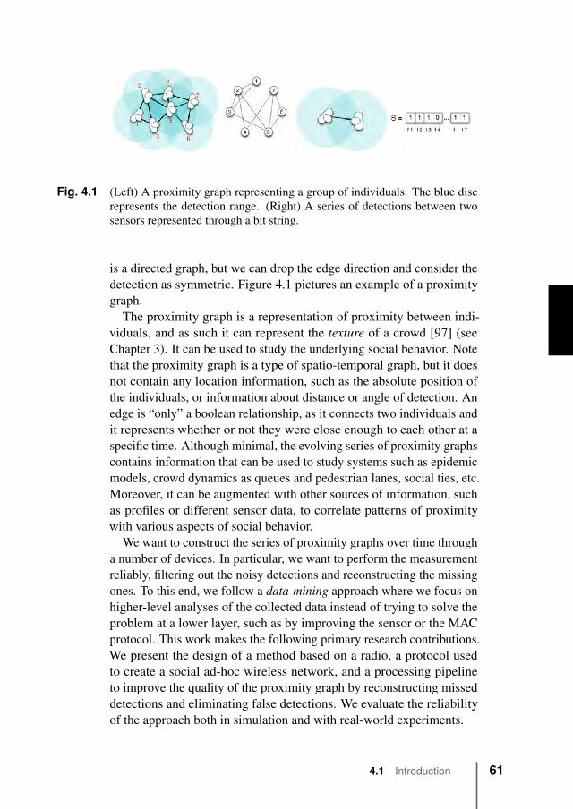
Fig. 4.1 (Left) A proximity graph representing a group of individuals. The blue discrepresents the detection range. (Right) A series of detections between twosensors represented through a bit string.

is a directed graph, but we can drop the edge direction and consider thedetection as symmetric. Figure 4.1 pictures an example of a proximitygraph.

The proximity graph is a representation of proximity between indi-viduals, and as such it can represent the texture of a crowd [97] (seeChapter 3). It can be used to study the underlying social behavior. Notethat the proximity graph is a type of spatio-temporal graph, but it doesnot contain any location information, such as the absolute position ofthe individuals, or information about distance or angle of detection. Anedge is “only” a boolean relationship, as it connects two individuals andit represents whether or not they were close enough to each other at aspecific time. Although minimal, the evolving series of proximity graphscontains information that can be used to study systems such as epidemicmodels, crowd dynamics as queues and pedestrian lanes, social ties, etc.Moreover, it can be augmented with other sources of information, suchas profiles or different sensor data, to correlate patterns of proximitywith various aspects of social behavior.

We want to construct the series of proximity graphs over time througha number of devices. In particular, we want to perform the measurementreliably, filtering out the noisy detections and reconstructing the missingones. To this end, we follow a data-mining approach where we focus onhigher-level analyses of the collected data instead of trying to solve theproblem at a lower layer, such as by improving the sensor or the MACprotocol. This work makes the following primary research contributions.We present the design of a method based on a radio, a protocol usedto create a social ad-hoc wireless network, and a processing pipelineto improve the quality of the proximity graph by reconstructing misseddetections and eliminating false detections. We evaluate the reliabilityof the approach both in simulation and with real-world experiments.

4.1 Introduction 61

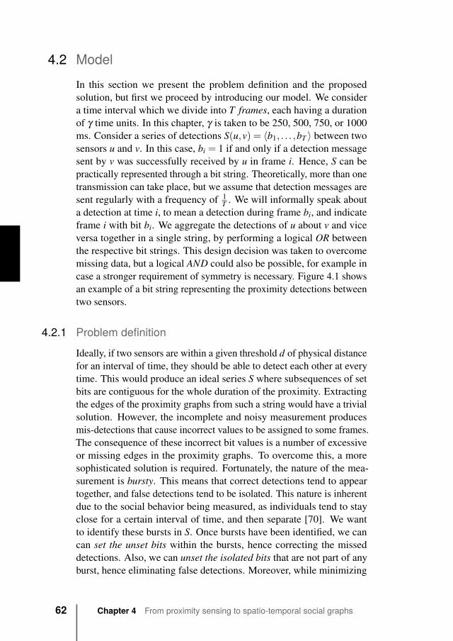
4.2 ModelIn this section we present the problem definition and the proposedsolution, but first we proceed by introducing our model. We considera time interval which we divide into T frames, each having a durationof γ time units. In this chapter, γ is taken to be 250, 500, 750, or 1000ms. Consider a series of detections S(u,v) = 〈b1, . . . ,bT 〉 between twosensors u and v. In this case, bi = 1 if and only if a detection messagesent by v was successfully received by u in frame i. Hence, S can bepractically represented through a bit string. Theoretically, more than onetransmission can take place, but we assume that detection messages aresent regularly with a frequency of 1

T . We will informally speak abouta detection at time i, to mean a detection during frame bi, and indicateframe i with bit bi. We aggregate the detections of u about v and viceversa together in a single string, by performing a logical OR betweenthe respective bit strings. This design decision was taken to overcomemissing data, but a logical AND could also be possible, for example incase a stronger requirement of symmetry is necessary. Figure 4.1 showsan example of a bit string representing the proximity detections betweentwo sensors.

4.2.1 Problem definitionIdeally, if two sensors are within a given threshold d of physical distancefor an interval of time, they should be able to detect each other at everytime. This would produce an ideal series S where subsequences of setbits are contiguous for the whole duration of the proximity. Extractingthe edges of the proximity graphs from such a string would have a trivialsolution. However, the incomplete and noisy measurement producesmis-detections that cause incorrect values to be assigned to some frames.The consequence of these incorrect bit values is a number of excessiveor missing edges in the proximity graphs. To overcome this, a moresophisticated solution is required. Fortunately, the nature of the mea-surement is bursty. This means that correct detections tend to appeartogether, and false detections tend to be isolated. This nature is inherentdue to the social behavior being measured, as individuals tend to stayclose for a certain interval of time, and then separate [70]. We wantto identify these bursts in S. Once bursts have been identified, we cancan set the unset bits within the bursts, hence correcting the misseddetections. Also, we can unset the isolated bits that are not part of anyburst, hence eliminating false detections. Moreover, while minimizing


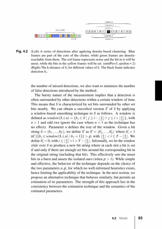
Fig. 4.2 (Left) A series of detections after applying density-based clustering. Blueframes are part of the core of the cluster, while green frames are density-reachable from them. The red frame represents noise and the bit in it will beunset, while the bits in the yellow frames will be set. (minPts=3, epsilon = 2)(Right) The k-distance of bi for different values of k. The black frame indicatesdetection bi.

the number of missed detections, we also want to minimize the numberof false detections introduced by the method.

The bursty nature of the measurement implies that a detection isoften surrounded by other detections within a certain window of time.This means that S is characterized by set bits surrounded by other setbits nearby. We can obtain a smoothed version S′ of S by applyinga window-based smoothing technique to S as follows. A window isdefined as window(S, i,n) = {b j ∈ S | j ≥ i−bn

2c∧ j ≤ i+ bn2c}, with

n > 1 and odd (we ignore the case where n = 1 as the technique hasno effect). Parameter n defines the size of the window. Given a bitstring S = 〈b1, . . . ,bT 〉, we define S′ as S′ = 〈b′1, . . . ,b′T 〉 where b′i = 1iif ‖{b j ∈ window(S, i,n) | b j = 1}‖> ρ , with bn

2c< i≤ T −bn2c. We

define b′i = 0, with i≤ bn2c∨ i > T −bn

2c. Informally, we let the windowslide over S to produce a new bit string where at each slot a bit is setif and only if there are enough set bits around the corresponding bit inthe original string (including that bit). This effectively sets the unsetbits in a burst and unsets the isolated ones (when ρ > 1). While simpleand effective, the behavior of the technique depends on the choice ofthe two parameters n,ρ , for which no well-informed heuristics exists,hence limiting the applicability of the technique. In the next section, wepropose an alternative technique that behaves similarly, but permits anestimation of its parameters. The strength of this approach lies in theconsistency between the estimation technique and the semantics of theestimated parameters.

4.2 Model 63

4.2.2 Density-based clustering

Given the bursty nature of S, we can use a density-based clusteringalgorithm and cluster dense subsequences of bits together. These clusterswould correspond to the bursts of detections we are looking for, whilethe outliers would correspond to the noisy detections to be ignored. Inparticular, we propose to use DBSCAN [55]. In S, the distance betweentwo bits bi and b j is defined as dist(bi,b j) = |i− j|. A bit bi is directlydensity-reachable from another bit b j if their distance is not more thanε (in that case it is said to be part of its ε-neighborhood) and if b j issurrounded by a sufficient number of bits to consider them a cluster,denoted as minPT S. A bit bi is called density-reachable from b j if thereis a sequence of bits b1, . . . ,bk, . . . ,bn with b1 = b j and bn = bi whereeach bk+1 is directly density-reachable from bk. Two bits bi and b j aredensity-connected if there is a third bit bk that is density-reachable fromboth. A cluster is a subset of S composed of mutually density-connectedbits, plus any bit that is density-connected to them. A point that is notpart of a cluster is considered noise. Figure 4.2 shows the result of theclustering algorithm on a series of detections between two sensors.

Analysis. One can see a correspondence between the window-basedsmoothing technique and the density-based clustering technique. Inboth cases, we identify bursts by thresholding the number of set bitswithin a certain “radius”, and we set the unset bits in the burst. In theformer, we set a bit in S′ if there are at least ρ set bits within a certaindistance, defined by the window size n, in the original string. In thelatter, we set the unset bits between density-reachable bits, which aresimilarly identified based on the minimum number of set bits minPTSwithin an ε-neighborhood. For this reason, one would expect to obtainsimilar results through the two techniques. Note that the application ofDBSCAN to our model affords a more efficient implementation thangeneral DBSCAN. The runtime complexity of general DBSCAN isO(N2), as each data point needs to be evaluated against all other datapoints to find its ε-neighbors. This runtime complexity can be reducedto O(NlogN) by means of an accelerated indexing structure such asa spatial index. In our model based on bit strings, collecting the ε-neighborhood of a bit has a constant cost as it requires to evaluate thebits within the ε-distance. As ε is fixed and evaluating a bit in a stringhas a constant cost, the cost of DBSCAN applied to our model is linearto the number of bits in the string. This makes the runtime cost of


the density-based clustering technique comparable to the cost of thewindow-based smoothing technique.

DBSCAN does not need any training phase and it does not require todefine a number of clusters in advance. However, it does require that thedata corresponds to a single density distribution function. In DBSCAN,the expected density distribution is defined through the parameters ε

and minPT S, and the algorithm is very sensitive to them. As we donot know the density distribution in advance, we need to estimate theseparameters. We propose such a technique in the next section.

4.2.3 K-nearest neighbors analysis

To study the density distribution of S we propose to compute the dis-tance within which a bit will find at least k bits, by also taking intoaccount that more bits can be at the same distance. By combining thisnotion of distance with the number of bits within that distance, we canestimate density. In particular, we propose to compute the distance ofthe k-Nearest Neighbors (k-NN), denoted as k-distance(bi). Given thedefinition of dist(bi,b j), the k-distance of detection bi is the δ suchthat:

(i) ‖{b∗ | b∗ = 1∧dist(bi,b∗)≤ δ}‖ ≥ k.(ii) ‖{b∗ | b∗ = 1∧dist(bi,b∗)< δ}‖< k.‖{b j, . . . ,bk}‖ denotes the cardinality of the set and hence the numberof detections. Figure 4.2 shows the result of the k-NN analysis run on aseries of bits.

Computing the k-distance of each detection in the string permits anoverview over the relationship between distance and neighborhood size.These in turn relate to the two parameters of DBSCAN ε and minPT S.In fact, the k-distance of bi is the ε necessary to collect at least k otherdetections around it. As such, it can be used to select the correct ε

that satisfies minPT S for the detections in the bursts. Usually, minPT Sis known in advance and is bounded to the definition of a cluster andthe noise in the data, and it can be used as a basis for the value of k.With large enough clusters, the detections should present a commonk-distance that corresponds to a representative density of the clusters,except for the noise or the members of clusters smaller than k. Selectingan ε that is close to this common k-distance guarantees that DBSCANwill cluster the detections together with the others within the k-distance.

4.2 Model 65

The k-distance plot1 is a means to study a k-distance distribution. Thisplot is constructed as follows. For a particular value of k, the k-distancefor each point is computed. These values are sorted in ascending order.The sorted list of points is plotted on a Cartesian plane, by using thek-distance value as the y coordinate and the position in the sorted list asthe x coordinate. We will use and show k-distance plots in the evaluationsections, to select the DBSCAN parameters. Note that in this work weselected ε manually to show the impact of the different choices on thebehavior of the method. However, approaches have been proposed toselect ε automatically through a numerical analysis of the k-distanceplot [158].

4.2.4 Proposed solutionOur proposed solution to extract a series of proximity graphs from aseries of detections consists of the following steps. The detectionsare collected with their timestamps from each sensor, and they areaggregated and converted to a bit string representation. The k-NNanalysis is performed on all the bit strings together, by computing thek-distance of each detection in each string, and sorting all these valuestogether into a single list. At this point, depending on the technologybeing used to perform the measurement, usually a range of valid valuesof minPT S is known in advance and it is used as k to compute the k-distances. Finally, each bit string is clustered with the representativek-distance as ε and k as minPT S. The extracted clusters and noise areused to correct the mis-detections, and finally the series of proximitygraphs can be generated.

4.3 Evaluation in simulationIn this section we present the evaluation in simulation of our proposed so-lution. The objective of this evaluation is to validate whether the methodcan construct correctly a proximity graph in a controlled environment,in the face of both data loss and noise.

4.3.1 MethodologyFor a scenario, we selected a social environment where individuals walkaround and form groups dynamically, to simulate a social location such

1In the literature this is usually called k-distance graph, but we use the term plot toavoid confusion.


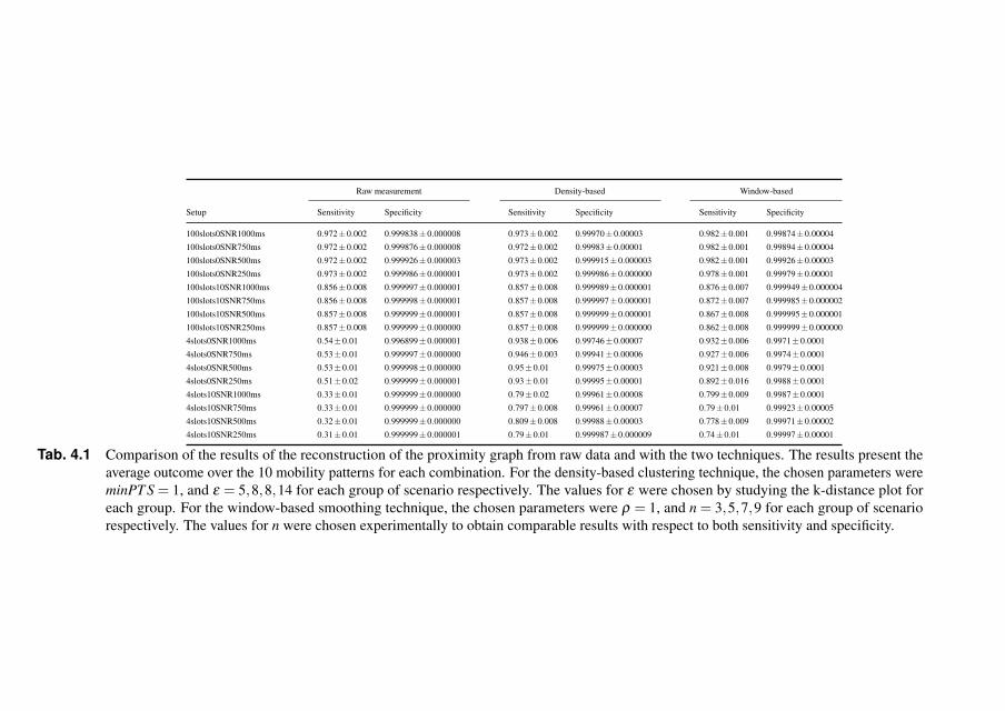
Raw measurement Density-based Window-based

Setup Sensitivity Specificity Sensitivity Specificity Sensitivity Specificity

100slots0SNR1000ms 0.972±0.002 0.999838±0.000008 0.973±0.002 0.99970±0.00003 0.982±0.001 0.99874±0.00004

100slots0SNR750ms 0.972±0.002 0.999876±0.000008 0.972±0.002 0.99983±0.00001 0.982±0.001 0.99894±0.00004

100slots0SNR500ms 0.972±0.002 0.999926±0.000003 0.973±0.002 0.999915±0.000003 0.982±0.001 0.99926±0.00003

100slots0SNR250ms 0.973±0.002 0.999986±0.000001 0.973±0.002 0.999986±0.000000 0.978±0.001 0.99979±0.00001

100slots10SNR1000ms 0.856±0.008 0.999997±0.000001 0.857±0.008 0.999989±0.000001 0.876±0.007 0.999949±0.000004

100slots10SNR750ms 0.856±0.008 0.999998±0.000001 0.857±0.008 0.999997±0.000001 0.872±0.007 0.999985±0.000002

100slots10SNR500ms 0.857±0.008 0.999999±0.000001 0.857±0.008 0.999999±0.000001 0.867±0.008 0.999995±0.000001

100slots10SNR250ms 0.857±0.008 0.999999±0.000000 0.857±0.008 0.999999±0.000000 0.862±0.008 0.999999±0.000000

4slots0SNR1000ms 0.54±0.01 0.996899±0.000001 0.938±0.006 0.99746±0.00007 0.932±0.006 0.9971±0.0001

4slots0SNR750ms 0.53±0.01 0.999997±0.000000 0.946±0.003 0.99941±0.00006 0.927±0.006 0.9974±0.0001

4slots0SNR500ms 0.53±0.01 0.999998±0.000000 0.95±0.01 0.99975±0.00003 0.921±0.008 0.9979±0.0001

4slots0SNR250ms 0.51±0.02 0.999999±0.000001 0.93±0.01 0.99995±0.00001 0.892±0.016 0.9988±0.0001

4slots10SNR1000ms 0.33±0.01 0.999999±0.000000 0.79±0.02 0.99961±0.00008 0.799±0.009 0.9987±0.0001

4slots10SNR750ms 0.33±0.01 0.999999±0.000000 0.797±0.008 0.99961±0.00007 0.79±0.01 0.99923±0.00005

4slots10SNR500ms 0.32±0.01 0.999999±0.000000 0.809±0.008 0.99988±0.00003 0.778±0.009 0.99971±0.00002

4slots10SNR250ms 0.31±0.01 0.999999±0.000001 0.79±0.01 0.999987±0.000009 0.74±0.01 0.99997±0.00001

Tab. 4.1 Comparison of the results of the reconstruction of the proximity graph from raw data and with the two techniques. The results present theaverage outcome over the 10 mobility patterns for each combination. For the density-based clustering technique, the chosen parameters wereminPT S = 1, and ε = 5,8,8,14 for each group of scenario respectively. The values for ε were chosen by studying the k-distance plot foreach group. For the window-based smoothing technique, the chosen parameters were ρ = 1, and n = 3,5,7,9 for each group of scenariorespectively. The values for n were chosen experimentally to obtain comparable results with respect to both sensitivity and specificity.

as a museum or a conference. Here we describe the different componentswe used to simulate our scenario and the metrics we used to evaluate theperformance of our solution.

Mobility patterns. We generated 10 mobility patterns with BonnMo-tion [8] using the Reference Point Group Mobility (RPGM) model [68]for a simulated crowd of 100 individuals moving for 60 minutes insideof a square arena of 25x25m. Each pattern was generated through adifferent random seed, but with the same set of parameters. The gener-ated patterns lead to a list of (x,y) coordinates describing where eachindividual will be at any given time. The individuals move with a speedof between 0.3 and 1.2 meters per second, but they can pause for upto 60 seconds. They form groups of a minimum size of 2 individualsand a maximum of 4, and when an individual comes in proximity ofa different group it will join the new group with a probability of 0.9.Each group has a semi-circular shape with an average diameter of 2meters. These parameters were chosen to simulate realistically the size,the inter-distance and the speed of movement of groups of individuals inthe desired scenario, while maximizing dynamicity.

Simulator. Each individual wears a simulated device. We simulatedthe devices in accordance with the devices we used for our real worldevaluation [45]. These nodes have an Atmel ATXMega128 CPU with8k of RAM, 128k of Flash memory, and a Nordic nRF24L01+ wire-less radio. To simulate the wireless network we used the OMNeT++2

simulation engine with the MiXiM3 framework for wireless and mobilenetwork, the de-facto simulation environment for mobile ad-hoc andsensor networks [146]. The devices form an ad-hoc wireless networkthrough an extension to the GMAC protocol [44]. In perfect conditions,the simulated transmission range is some 3.5 meters. For our purposes,we influenced these conditions in multiple ways through the simulatorand protocol parameters.

Metrics. We extracted a series of proximity graphs directly from thecoordinates of each mobility pattern and we consider these as our groundtruth. We used a distance range of 3.5 meters to construct the proximitygraph, as this is the ideal transmission range of our simulated devices.

2http://www.omnetpp.org3http://mixim.sourceforge.net


To measure the performance of our proposed solution we compute thenumber of:

• false positives (FP): detections that are present in the measuredproximity graph but not in the ground truth.

• false negatives (FN): detections that are present in the groundtruth but not in the measured proximity graph.

• true positives (TP): detections that are present in the measuredproximity graph and in the ground truth.

• true negatives (TN): detections that are missing in the measuredproximity graph and in the ground truth.

We use these tests to compute two statistical measures of perfor-mance for binary classification tests. Sensitivity can be used to mea-sure the ability of the test to identify positive results and is defined assensitivity= T P

T P+FN . Specificity can be used to measure the ability of thetest to identify negative results and is defined as speci f icity = T N

T N+FP .Intuitively, they measure the ability of the sensor to detect correctlyproximity and the absence of it, respectively.

4.3.2 SetupsAccording to our approach, each sensor periodically broadcasts its IDthrough the radio, and a reception of such a transmission is consideredas a detection. There are three main parameters we used to influencethe behavior of the wireless network, and as such of the detections. Weevaluated each of the 16 combinations of the three parameters over allthe 10 mobility patterns, for a total of 160 simulation runs.

First, we can choose the number of slots used by the GMAC layer forthe broadcasts. In GMAC, time is divided into a sequence of frames,and each frame is composed of a number of slots. The slot allocationalgorithms of GMAC are based on Slotted Aloha [3], and are used toshare access to the wireless medium. At a high level, the main differencebetween GMAC and Slotted Aloha is that GMAC exploits duty cycling.Slotted Aloha is an always-on protocol, whereas GMAC turns the radioon only for a small percentage of the total slots in order to save energy.Slots in which the radio is powered up are known as active slots, incontrast to inactive, or idle slots, where the radio is powered down.By controlling the number of active slots and their allocation strategy,we can control the number of “collisions” when multiple sensors arewithin the range d, and hence of loss of detections. In particular weexperimented with the 4slots setup, where four randomly allocatedactive slots are used (introducing a large number of collisions), and the

4.3 Evaluation in simulation 69

100slots setup, where each node has a slot assigned statically accordingto its ID (ideally avoiding collisions completely).

Second, radio irregularity can introduce variations in packet receptionand it can be caused by factors related to the device and to the medium.Examples of the first ones include the antenna type, the transmissionpower, antenna gains, receiver sensitivity, receiver threshold and theSignal-to-Noise Ratio (SNR). Factors related to the medium are themedium type, the background noise, and some other environmentalfactors, such as the temperature and obstacles within the propagationmedia [169, 1]. While simulating some of the medium factors is morecomplicated, most of these factors are considered explicitly by thesimulation engine [80], including those specific to the characteristics ofour devices. Here, we concentrate in particular on the SNR, relaxingthe assumption of a uniform disc of transmission and reception. Weexperimented with the 10SNR setup, where a SNR threshold of 10 isused, and the 0SNR setup, where the threshold is completely ignored.

Third, the frame length is expressed in time units, and it defines theperiodicity with which nodes broadcast their ID. It defines the rate atwhich detections are collected. This rate acts as a sampling rate forour sensor, and it should be chosen according to the dynamicity of thebehavior to be measured. For instance, it is desirable to use a framelength a number of times shorter than the minimum amount of time twosensors can be in each other’s proximity. This allows to obtain potentiallymultiple detections during that interval and overcome possible loss ofdetections. We will show that increasing the sampling rate is veryimportant to filter out noise. On the other hand, a higher sampling rateincreases energy consumption, as the radio is used more frequently.There is a trade-off between energy efficiency and the sensitivity of theinstrument. We experimented with the 1000ms, 750ms, 500ms, 250mssetups, which use a frame length as their name suggests.

4.3.3 ResultsWe ran the 160 runs of simulation and computed the sensitivity and speci-ficity of the proximity graphs extracted from the raw measurements, andobtained through window-based smoothing and density-based clustering.Table 4.1 shows the results. For the raw measurement, the sensitivitysimply measures the number of recorded detections, as it represents thenaive approach that uses only set bits for the construction of the edges.For the raw measurement, two things should be noted. First, changingthe number of slots and the allocation algorithm causes nearly 50% of


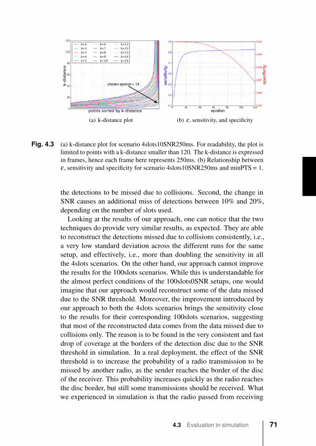
(a) k-distance plot (b) ε , sensitivity, and specificity

Fig. 4.3 (a) k-distance plot for scenario 4slots10SNR250ms. For readability, the plot islimited to points with a k-distance smaller than 120. The k-distance is expressedin frames, hence each frame here represents 250ms. (b) Relationship betweenε , sensitivity and specificity for scenario 4slots10SNR250ms and minPTS = 1.

the detections to be missed due to collisions. Second, the change inSNR causes an additional miss of detections between 10% and 20%,depending on the number of slots used.

Looking at the results of our approach, one can notice that the twotechniques do provide very similar results, as expected. They are ableto reconstruct the detections missed due to collisions consistently, i.e.,a very low standard deviation across the different runs for the samesetup, and effectively, i.e., more than doubling the sensitivity in allthe 4slots scenarios. On the other hand, our approach cannot improvethe results for the 100slots scenarios. While this is understandable forthe almost perfect conditions of the 100slots0SNR setups, one wouldimagine that our approach would reconstruct some of the data misseddue to the SNR threshold. Moreover, the improvement introduced byour approach to both the 4slots scenarios brings the sensitivity closeto the results for their corresponding 100slots scenarios, suggestingthat most of the reconstructed data comes from the data missed due tocollisions only. The reason is to be found in the very consistent and fastdrop of coverage at the borders of the detection disc due to the SNRthreshold in simulation. In a real deployment, the effect of the SNRthreshold is to increase the probability of a radio transmission to bemissed by another radio, as the sender reaches the border of the discof the receiver. This probability increases quickly as the radio reachesthe disc border, but still some transmissions should be received. Whatwe experienced in simulation is that the radio passed from receiving


everything to nothing. This basic on/off behavior is to be expected inabsence of interference [109].

In effect, the SNR threshold causes the detection range to simplyshrink. This hypothesis is confirmed by the absence of improvementwhen the frame length is decreased in the 10SNR scenarios. In fact, witha higher detection rate and without this on/off behavior, one would ex-pect a higher chance that at least a few detections would make it throughthe disc border. Fortunately, this behavior is expected only in simula-tion, as it has been shown that the behavior of real links in low-powerwireless networks, such as ours, deviates to a large extent from the idealbinary model used in several simulation studies. In particular, there is alarge transitional region in wireless link quality that is characterized bysignificant levels of unreliability and asymmetry [164]. In the remainderof this chapter, we stick to the density-based clustering technique only,as it allows for an estimation of its parameters through the K-nearestneighbors analysis.

Choosing epsilon. To obtain the results presented in Table 4.1, wehave carefully chosen the values for ε by using the k-distance plot as areference. Figure 4.3(a) shows one of these plots and in particular theplot for our most realistic scenario 4slots10SNR250ms, for k = 1, . . . ,15.For small values of k, the plot presents lines with a slope characterizedby points with low k-distance values, and whose gradient changes onceand very quickly towards the end. The points in the part of the curvewith a low slope represent detections inside of clusters, and their k-distance value is the distance from their k-NNs. Note that all curves areconsistently bimodal, meaning that the data presents a single densitydistribution, as expected and as required by DBSCAN. For readability,the plot presents only points with k-distance values under 120, but thedata presents points with k-distance up to around 10000. These are thepoints that represent the distance between two detections that happenedduring two distinct and temporally distant moments. The k-distance isexpressed in frames, so a k-distance of 1 represents 250ms.

To choose ε with k = 1, we concentrated on the elbow of the curvewhere the slope increases quickly, i.e., between k-distance 10 and 20 (forour experiments we chose a prudent value of 14 to preserve specificity).The points in this range represent detections that are in the sparse areasof the clusters or at their boundaries. Their k-distances are good can-didates for our choice of ε . One has to be careful though, as a larger ε

increases the probability to merge adjacent clusters. When this happens,


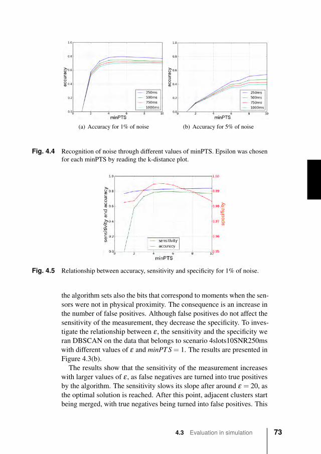
(a) Accuracy for 1% of noise (b) Accuracy for 5% of noise

Fig. 4.4 Recognition of noise through different values of minPTS. Epsilon was chosenfor each minPTS by reading the k-distance plot.

Fig. 4.5 Relationship between accuracy, sensitivity and specificity for 1% of noise.

the algorithm sets also the bits that correspond to moments when the sen-sors were not in physical proximity. The consequence is an increase inthe number of false positives. Although false positives do not affect thesensitivity of the measurement, they decrease the specificity. To inves-tigate the relationship between ε , the sensitivity and the specificity weran DBSCAN on the data that belongs to scenario 4slots10SNR250mswith different values of ε and minPT S = 1. The results are presented inFigure 4.3(b).

The results show that the sensitivity of the measurement increaseswith larger values of ε , as false negatives are turned into true positivesby the algorithm. The sensitivity slows its slope after around ε = 20, asthe optimal solution is reached. After this point, adjacent clusters startbeing merged, with true negatives being turned into false positives. This


is evident by the specificity curve that starts decreasing around that samevalue of ε . These results show that good values of ε can be chosen by acorrect read of the k-distance plot. Similar results can be obtained withlarger values of minPT S. Note that the k-distance plot is often the onlyinstrument available to estimate ε , as the measurement of sensitivity andspecificity requires ground truth data.

Filtering out noise. Until now, we have kept minPT S fixed to 1, sothat also single detections could generate edges in the proximity graph.In a scenario where isolated detections can be generated by corruptionsand interferences to the signal, a larger value might be necessary. Thisway, DBSCAN requires a larger minimum number of detections toestablish a cluster, and this enables it to recognize noise. The downsideis that short intervals of physical proximity risk to be filtered out as well,when the number of detections that characterize them is smaller thanminPT S. This problem is particularly relevant for larger frame lengths,as they produce a lower detection rate and hence less detections for thesame interval of time.

To investigate this hypothesis, we injected artificial noise into the datagenerated by the simulators. We ran three experiments where we set1%, 5% and 10% of the bits in each bit string, respectively. For eachpair of nodes, the bits were chosen uniformly at random. Each test wasrepeated 10 times and the results in Figure 4.4 and Figure 4.5 show theaverage values of accuracy in identifying the injected noise. The plotsdo present error bars, but due to the very low standard deviation they arenot visible.

The results show that for 1% of noise the algorithm is able to recognize80% of the noise already with a minPT S of 4. For the experiment with5%, 60% of the noise is recognized correctly with a minPT S of 10.We do not present results for the experiment with 10% of noise aswith minPT S of 10 the accuracy was below 1%. These results validateour hypotheses. In fact, by specifying a larger value for minPT S weare able to recognize an increasing amount of noise. Moreover, byincreasing the detection rate the algorithm is able to recognize morenoise, i.e., a difference of 10% between the 1000ms and 250ms framelength respectively. Note that, in particular with higher rates of noise,some of the randomly selected bits might be already set or belong toalready existing bursts, hence not producing actual noise. This meansthat a 100% accuracy is an unrealistic result to reach. Overall, theresults of these experiments show that, for realistic noise rates, the


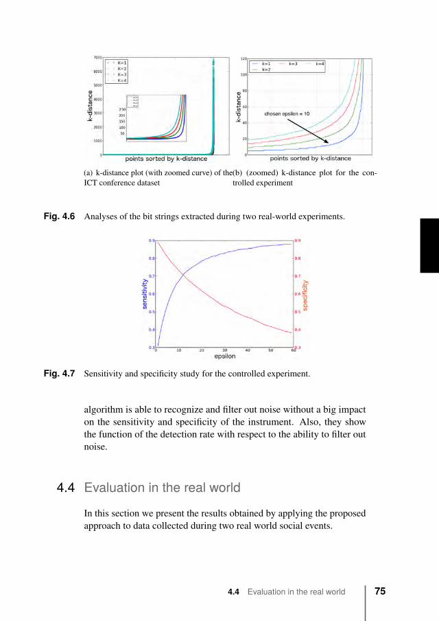
(a) k-distance plot (with zoomed curve) of theICT conference dataset

(b) (zoomed) k-distance plot for the con-trolled experiment

Fig. 4.6 Analyses of the bit strings extracted during two real-world experiments.

Fig. 4.7 Sensitivity and specificity study for the controlled experiment.

algorithm is able to recognize and filter out noise without a big impacton the sensitivity and specificity of the instrument. Also, they showthe function of the detection rate with respect to the ability to filter outnoise.

4.4 Evaluation in the real world

In this section we present the results obtained by applying the proposedapproach to data collected during two real world social events.

4.4 Evaluation in the real world 75

4.4.1 MethodologyTo explore the behavior of our approach on real data, we measuredproximity information at two social events. In particular, we first con-ducted a controlled experiment in our laboratory, where we collectedboth proximity information and ground truth. Afterwards, we conducteda large-scale experiment during an IT conference attended by around 250individuals. The devices were running the same software and protocol asthe virtual devices in our simulations, and were hence using the GMACprotocol to broadcast their IDs every second to a short distance of 2-3meters. Every device recorded the list of IDs received by the sensorat each second in the on-board storage unit, and we later collected thisdata for our offline analyses. The sensors were using 64 active slotsand would choose randomly which slot to use to broadcast their ID.This combination represents a compromise between the 100slots and4slots simulated setups. The devices were also broadcasting a secondtype of transmission. In fact, between two short-range transmissions,a long-range transmission was broadcast up to about 20 meters. Thissecond broadcast contained the list of IDs received by each device dur-ing the previous frame, hence comprising only short-range detections.We captured these long-range transmissions through stationary devicescalled “sinks”. Sinks capture the radio transmissions exchanged by thedevices, but do not transmit any data over the ad-hoc wireless network.We used this data to visualize at the events the evolution of the proximitygraphs in real-time. Long-range transmissions were not used to detectproximity.

4.4.2 Evaluation against ground truth dataWe conducted a first experiment in a controlled environment to collectground truth data about physical proximity. For the experiment, 12individuals participated to a cooperative social game in our laboratory.The experiment lasted about 45 minutes and was designed to replicatea conference hall scenario. The game required the individuals to formgroups and interact to solve a quiz. At any time the individuals couldswitch groups, mimicking the way people switch conversations during acoffee break. During the experiment, the individuals were wearing ourbadge devices on their chest, in a similar way as a typical conferencebadge is worn. In addition to our badges, we used a real-time locationsystem (RLTS) 4 to track the position of each individual at each time.

4Ubisense: http//www.ubisense.net


Moreover, we annotated the evolution of the formation of the groupsthrough 5 video cameras and a human observer. From these two sources,we extracted two ground truth data sets.

Results. We performed the study of the sensitivity and the specificityof our proximity measurements against both ground truth data sets.The results were consistent with both ground truth sets but, due tospace constraints, we report in Figure 4.7 only the results against theRLTS data, as it was a harder task. In fact, when our badge is wornon the chest, the body partially shields the transmissions, biasing thesensing area towards the front. On the other hand, the ground truth wasextracted from the RLTS following the assumption of a uniform disc.As a result, some detections might be missed by our badges (e.g., whentwo individuals stand back to back), decreasing the sensitivity of themeasurement. Reading the k-distance plot shown in Figure 4.6(b), wechose for ε a value of 10. The validity of the choice is confirmed by thestudy of the sensitivity and specificity for different values of ε shownin Figure 4.7. Precisely, using our approach with this parameter thesensitivity of the measurement improved from 0.309 (raw measurement)to 0.670, while the specificity decreased from 0.890 (raw measurement)to 0.733. Similar results were obtained against the annotated groundtruth (sensitivity from 0.389 to 0.792 and specificity from 0.908 to0.759). These results are strongly consistent with our simulations, as thesensitivity is more than doubled in the face of a decrease in specificityof only around 17%. This confirms the effectiveness of our approachalso in a real-world scenario and make us confident of the quality of themeasured proximity graphs.

4.4.3 Evaluation at an ICT conference

We conducted a second experiment at an ICT conference attended byaround 250 individuals, 137 of which were wearing one of our devices.The conference presented six different tracks, and the track rooms wereall scattered around the main hall of the event location. This main hallhosted the coffee breaks, the lunch banquet, and the poster session. Werecorded proximity information for the whole event, but here we focuson the two hours between 12:00 and 14:00 when the lunch banquet andthe poster session took place. No talks were given during this period,and the individuals were all gathered in the main hall. Due to the natureand the scale of the experiment, it was not possible to collect groundtruth data.

4.4 Evaluation in the real world 77

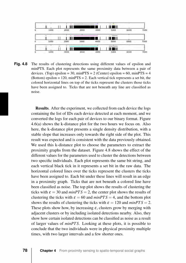
Fig. 4.8 The results of clustering detections using different values of epsilon andminPTS. Each plot represents the same proximity data between a pair ofdevices. (Top) epsilon = 30, minPTS = 2 (Center) epsilon = 60, minPTS = 4(Bottom) epsilon = 120, minPTS = 2. Each vertical tick represents a set bit, thecolored horizontal lines on top of the ticks represent the clusters those tickshave been assigned to. Ticks that are not beneath any line are classified asnoise.

Results. After the experiment, we collected from each device the logscontaining the list of IDs each device detected at each moment, and weconverted the logs for each pair of devices to our binary format. Figure4.6(a) shows the k-distance plot for the two hours we focus on. Alsohere, the k-distance plot presents a single density distribution, with astable slope that increases only towards the right side of the plot. Thisresult was expected and is consistent with the data previously obtained.We used this k-distance plot to choose the parameters to extract theproximity graphs from the dataset. Figure 4.8 shows the effect of thedifferent values for the parameters used to cluster the detections betweentwo specific individuals. Each plot represents the same bit string, andeach vertical black tick in it represents a set bit in the raw data. Thehorizontal colored lines over the ticks represent the clusters the tickshave been assigned to. Each bit under these lines will result in an edgein a proximity graph. Ticks that are not beneath a colored line havebeen classified as noise. The top plot shows the results of clustering theticks with ε = 30 and minPT S = 2, the center plot shows the results ofclustering the ticks with ε = 60 and minPT S = 4, and the bottom plotshows the results of clustering the ticks with ε = 120 and minPT S = 2.These plots show how, by increasing ε , clusters grow by merging withadjacent clusters or by including isolated detections nearby. Also, theyshow how certain isolated detections can be classified as noise as a resultof larger values of minPT S. Looking at these plots, it is possible toconclude that the two individuals were in physical proximity multipletimes, with two larger intervals and a few shorter ones.


When designing an instrument that will be deployed to real environ-ments, sources of mis-detections should be considered with high priority.During the experiment, we also measured the radio transmissions with aspecial device called an RF sniffer. This device scans a tunable band ofradio frequency waves and attempts to interpret the observed signals aspackets at high resolution. Where a normal device will observe nothingin the event of two messages colliding, an RF sniffer will observe somecombination of the two messages generated by the overlapping of thetwo individual radio signals. As such, this device allows us to makesome observations about the number of collisions/corrupt packets thatwould be experienced by devices in the vicinity of this sniffer. Duringthe experiment our RF sniffer observed 277764 packets. Of these pack-ets, 137077 were valid and 140687 (or just over 50%) were corrupt.These corrupt transmissions could be the result of many factors (e.g.,interference from nearby WiFi devices), but the most likely cause ismessage collisions with other devices. These collisions will result inmissed detections. In addition, it is likely that some corrupt packets(incorrectly) passed the CRC check, resulting in being accepted as validdata. The effect of these messages would be false positives, as the cor-rupt data would cause the device to detect other devices that are not trulyat distance range, for example by modifying the transmitted ID withthe ID of another device due to a flipped bit. These statistics show thenecessity for a method such as ours to cope with these effects.

4.5 Discussion

We have shown how the application of data mining techniques to datacollected through a number of wearable sensors can increase the relia-bility and the accuracy of physical proximity measurements. We havealso shown how the setting of the parameters can influence sensitivityand specificity. In particular, trying to increase sensitivity exceedinglycan cause specificity to decrease. Using an overly large value for ε cancause true negatives to be turned into false positives. Hence, there is atrade-off between the number of false negatives that can be turned intotrue positives and the number of true negatives that will be turned intofalse positives. It depends on the different applications and algorithmswhether false negatives should be preferred to false positives and viceversa, putting the choice in the hands of practitioners. Regardless of thischoice, one cannot assume a filtering of the data that yields to a perfectreconstruction of the measurement. In fact, algorithms and applications

4.5 Discussion 79

should be designed to cope with unreliable and inaccurate data, insteadof assuming perfect measurements.

The presented approach assumes a single density distribution of de-tections that is valid for all pairs of devices at each time. While thisassumption is reasonable for scenarios such as those described in thischapter, where the density distribution of individuals in space tends to beuniform and stable, more dynamic scenarios and longer measurementsrequire a refinement of our approach. For example, individuals locatedin highly dense areas will experience a higher rate of false negativesand will require a larger ε . The same individuals, at a different time,might experience a lower rate in areas characterized by lower density.For this reason, for our future work we plan to extend our techniqueto consider data collected only during a limited amount of time, andadapt the estimate of ε accordingly. Moreover, we plan to investigate astream-based technique that will allow us to consider only these most re-cent measurements in an online fashion. Ultimately, this more localizedapproach should enable the integration of the techniques directly on thedevices.

4.6 Related work

Extracting proximity information about social behavior with on-bodysensors is not a new idea. The Sociometer [32] is a wearable device thatcan measure social signals through IR sensors, microphones, Bluetooth,accelerometers, etc. As the focus of the Sociometer is to measure face-to-face interactions, proximity is sensed within a narrow frontal cone-shaped region of up to two meters. Given that people move around whenthey are talking, also the Sociometer suffers from bursty measurements.For this reason, the data extracted from the four IR sensors is processedwith a Hidden Markov Model that is trained to learn patterns of IRsignals over an annotated dataset. The focus on a frontal measurementand the dependence on annotated data pushed us to pursue a differentapproach. Hitachi’s Microscope [159] is a device that provides similarfeatures to those characterizing the Sociometer.

In [74] an approach based on RFIDs is presented. Similar to ourapproach, the device is worn on the chest of the individuals, and thedevices periodically exchange their IDs through radio packets to detectphysical proximity at close range. One of such detections accounts foran interval of proximity of 20 seconds. According to the authors, thedevices operate with parameters that can assess physical proximity with


a probability in excess of 99% over such time interval. As the parametersand the method are not described, it is difficult to identify the reliabilityof this assessment. Moreover, we aim at a more sensitive measurementthan the one provided over those 20 seconds of potential false positives.

A different approach is followed for the iBadge [107]. The iBadge isa wearable device that can measure location, orientation and tilt, envi-ronmental settings, and speech. Orientation and tilt are measured fromacceleration and magnetic sensors. The localization process is based onthe location knowledge of fixed beacons (devices with known location)attached to the ceilings and the ability of the iBadge to accurately mea-sure the distance between itself, the fixed beacons, and other iBadgesin the room. The distance is measured by recording the arrival timedifference of a simultaneous transmission of an RF signal and an ultra-sonic burst. Using the distance measurements from multiple beacons inthe room, iBadge estimates its precise 3-D location. Although iBadgescooperate in this localization process, the measurement of physical prox-imity is based on beacons. We consider this approach limiting andprefer a decentralized approach that does not need or produce locationinformation.

4.7 ConclusionsIn this work we have presented a method to sense physical proxim-ity reliably. The method is based on a miniaturized device runningan energy-efficient protocol for social ad-hoc wireless networks. Theinstrument can operate for weeks with one battery charge, making itsuitable for long studies. The detections extracted from the network canbe processed through a data mining technique that reconstructs misseddetections and filters out noise. We evaluated both in simulation and inreal-world experiments that the approach is able to increase the sensitiv-ity of the sensor without lowering its specificity too much. The approachdoes not require a learning phase, but only a few parameters. We haveprovided a non-parametric method to choose the values for these param-eters. The method provides a reliable measurement of proximity that isnot bounded to the particular technology used to sense physical prox-imity, and can hence be used in a variety of scenarios and applications.Our approach is not specific to our devices or to a particular medium,but it is applicable to different technologies and protocols, as long asthe technological layer underneath can map onto the proposed binarymodel.

4.7 Conclusions 81

5Leveraging proximity sensing tomine the behavior of museumvisitors

„Without data, you are just anotherperson with an opinion.

— Andreas Schleicher

5.1 IntroductionIn the previous chapters we have discussed how person-to-person prox-imity detections can be leveraged to study crowd behavior. However,face-to-face proximity is not the realm of solely person-to-person re-lationships, but it can be used as a proxy to study person-to-objectrelationships as well. In fact, we face the objects with which we inter-act on a daily basis, like a television, the kitchen appliances, a book,including more complex objects like a stage where a concert is takingplace. In this chapter, we focus on the relationship between the visitorsof an art exhibition and its exhibits. We design, implement, and deploya sensing infrastructure based on inexpensive mobile proximity sensorsand a filtering pipeline that we use to measure face-to-face proximitybetween individuals and exhibits. Furthermore, we leverage person-to-object relationships to understand crowd behavior by identifying andpredicting group behavior, which we visualize to gain insights into thebehavior of the crowd.

Museum staff design exhibitions to educate, engage and entertainthe visitors. Yet, museums rely on surveys and expensive observational

The contents of this chapter have been originally published in “Leveraging proxim-ity sensing to mine the behavior of museum visitors” C. Martella, A. Miraglia, M.Cattani, M. van Steen - IEEE International Conference on Pervasive Computing andCommunications PERCOM 2016 and “Visualizing, Clustering, and Predictingthe Behavior of Museum Visitors” C. Martella, A. Miraglia, J. Frost, M. Cattani,M. van Steen - Pervasive and Mobile Computing 2016, and have been slightlymodified to improve readability.

83

studies to collect coarse-grained information about the response of theirvisitors, with limits of scalability and bias. Central to the understandingof how visitors interact with an exhibition is the identification of whichexhibits individuals stop at, for how long, and in which order. Accordingto an ethnographic observational study of visiting styles at the Louvremuseum, visitors can be classified into four classes according to theirmovements [140]. For example, one class of visitors follows a specificpath spending a lot of time at almost all exhibits, while another classseems to have a specific preference for some known exhibits at whichthey spend a lot of time, ignoring the others. This classification hasbeen used, based on activity logs coming from a digital museum guide,to help engage museum visitors and avoid information overload [82].Characterizing and quantifying visitors behavior helps museum staffevaluate their curatorial decisions, reporting to stake holders and funders,and building data-driven marketing campaigns and applications.

The key to collecting this information is the fine-grained measurementof face-to-face proximity between visitors and exhibits. We call posi-tioning the problem of identifying which exhibit an individual is facingat short distance. Existing approaches are not suitable for this problem.Indoor localization technologies estimate the absolute position of anindividual in space, without measuring where the individual is looking at.This means that positioning an individual at the closest artwork withina given distance can produce false positives if the individual has herback towards the exhibit or if she is facing an artwork nearby. Moreover,only very few existing state-of-the-art techniques achieve, in optimalcontrolled environments, an error of less than 2 meters. With such errors,positionings of the visitor at a wrong exhibit, including those at the otherside of a wall, would be frequent. Finally, these techniques often requireexpensive investments and rely on complex setup procedures each timeexhibits are re-arranged.

Contributions. In this chapter, we propose a technique based on inex-pensive and energy-efficient mobile proximity sensors, and a filteringpipeline to accurately position visitors at exhibits at all times. While weuse radio-based proximity sensors, our filtering pipeline is not bound toany particular technology and does not require, for example, measuringdistance from exhibits or expensive setups. In particular, we introducea particle filter tailored to the problem of positioning, together withtwo smoothening filters that increase measurement accuracy. We usepositionings to reconstruct the time spent at exhibits and the visitor path,

84 Chapter 5 Leveraging proximity sensing to mine the behavior of

museum visitors

defined as the ordered sequence of exhibits visited by the individual. Weevaluate the approach with data collected from 182 volunteers duringa real-world experiment. We show that by clustering this data we canidentify and predict group behavior, such as common paths and patternsof time distribution at exhibits. Moreover, we show that by visualizingthe behavior of the crowd we can help museum stuff gain a better un-derstanding of the response of the crowd to their decision-making andplanning.

The remainder of this chapter is organized as follows. First, we givean overview of our system, including sensing infrastructure, filteringpipeline, and data analysis. Then, we discuss related work regardinglocalization systems and museum technology. After describing ourmodel and pipeline, we evaluate the accuracy of our measurements. Wecontinue by presenting a number of visualizations of the data, and byapplying state-of-the-art data mining techniques to the data. Finally, weconclude with a discussion about limitations and future work.

5.1.1 MotivationBefore deploying our infrastructure and running our data-collectionexperiment at the museum, we conducted a series of semi-structuredinterviews with the curator, the artistic director, and the head of businessdevelopment to better understand their processes and needs. In additionto the staff of CoBrA, we also interviewed an independent exhibitiondesigner who works regularly at CoBrA, and an administrator from thevan Gogh museum who commissioned a large-scale observational studyof that museum and has applied the findings to the re-organization ofthe permanent exhibition. Interview notes were coded and themes wereidentified. The analysis revealed three themes.

Inform design of future shows. Currently, museum staff designsexhibitions based on theories and experience about what pieces arepopular and how visitors will move through the gallery spaces. Forexample, the artistic director at CoBrA believes that wall placementmay impact visitors’ movement through a show more than the displayedartworks, but expects that visitors also deviate from the ordering thatcurators envision. Both creative staff and those in charge of businessdevelopment at CoBrA expressed a need for objective information to testsuch assertions and improve intuitive understanding about the gallery.The artistic director stated “If we learn more about that flow, [it] willhave an impact on how we design, how we display the works of art.”

5.1 Introduction 85

Within a larger institution, the van Gogh Museum, parts of the gallerieswere redesigned based on the results of an observational study. The studyhad identified that the previous placement of certain famous artworkswere causing congestion in parts of the gallery space. Moreover, lesspopular pieces were ignored when positioned close to more popularones. Finally, the position of some divider walls confused some visitorsabout what path they were expected to follow in the museum, resultingin some parts of the exhibition being skipped completely. As we show inthis chapter, similar observations — in fact corresponding visualizations— can be obtained with our sensor-based system, at a much lower cost.

Report to funders and potential partners. For the last ten years, thehead of business development at the CoBrA has received requests fromfunders to demonstrate the value of shows. He stressed the need for“quantifiable information” about the experience of visitors. Museumstrack some metrics: ticket sales, museum shop sales and some periodicsurveys, but these do not indicate how visitors interact with different art-works or level of satisfaction once inside of the exhibition. Specifically,the head of business development would like to know how much timevisitors spend viewing particular pieces and how they move through theshow. He wants to share these metrics externally in funding requestsand inform the design of marketing campaigns. Finally, he found that,for example, identifying most popular artworks during the first weeksof a new exhibition could help the design of the marketing campaign,perhaps based on those pieces.

Increase participation. In the museum world, the staff of CoBrAreports a concern that visitors can remain passive and fall into the“museum shuffle”, that is, visitors walk from piece to piece mindlessly,spending a few seconds at each piece before moving on. Museum staffwants to find ways to know when this occurs such that they can interveneand change behavior. The ultimate goal is to avoid this passive modeand enhance engagement with the content to increase the exhibitions“impact” beyond the visit itself. The interviewees’ main objective for amuseum visit is for visitors to learn something. To do so, they want to“get in touch” with visitors using different methods of understanding thevisitor experience. The artistic director acknowledged current methodswere not providing the right type of information: “we know them instatistics [. . . ] but we do not know about the quality of their experience”.


museum visitors

The results of these interviews were used for the design of our datacollection and data analyses.

5.2 OverviewWe conducted a 5-days experiment spread across 2 weekends at theCoBrA Museum of Modern Art (CoBrA). Our data collection focusedon the temporary exhibition entitled “The Hidden Picture”, a curatedsample of the corporate collection of ING. The exhibition was displayedin the dedicated open space at the top floor of the museum. The spaceis configurable, and divider walls were used to separate the space into6 “open rooms” dedicated to different themes. The overall space wasabout 100 meters long and 25 meters wide, with a ceiling reaching about5 meters, while divider walls were some 3.5 meters high.

Rooms 1 and 2 focused on figurative art, rooms 3 and 4 mostlyon abstract art, room 6 on pieces inspired by nature, for a total of 60pieces. The pieces varied in size, style and medium, including photos,paintings, sculptures, videos, and an installation with a cage hosting aliving chameleon. None of the pieces were highly famous, and werehence appealing the visitors based on immediate reaction rather than onprior knowledge. Of the 60 pieces, we instrumented 45 exhibits withour sensing infrastructure.

5.2.1 Data-collection architectureWe designed a system based on inexpensive radio-based proximity sen-sors. Our sensing solution is compliant to the Zigbee standard and itcan be implemented for example through Bluetooth low energy (BLE)beaconing, available in modern smart phones. To give us freedom toinvestigate our solution, instead we deployed ad-hoc devices running aduty-cycled MAC protocol [142] that allows us to run our system forweeks with a single battery charge.

The sensing infrastructure comprises mobile devices and anchorpoints (or simply anchors). Mobile devices are sensor nodes wornby the visitors. They are attached to a lanyard worn around visitors’neck and hang on the chest. Due to the shielding effect of the visitor’sbody, the radio communication range is steered to the front with a con-trolled angle of around 90 degrees and some 2-3 meters of distance.Anchors are sensor nodes positioned at the base of each exhibit. Weinstalled anchors inside of enclosure aluminum boxes designed to shapethe communication range to approximately 60 degrees and 2-3 meters of

5.2 Overview 87

distance. With this setup, mobile devices and anchors can communicateonly when the visitor is facing an exhibit.

Every second, anchors transmit through the radio a unique anchoridentifier (AID) that is received and timestamped by mobile deviceswithin range. We consider the reception of an AID by a mobile device aproximity detection. Note that our sensors do not measure radio signalstrength (i.e., RSSI). While it does not enable us to measure distancebetween points, it allows a cheaper and more energy-efficient solution.Every second, mobile devices transmit the list of detections receivedduring the previous second together with their unique mobile-pointidentifier (MID) to a longer range of approximately 100 meters, whichare received by one or more sinks.

Sinks are computers that receive mobile devices transmissions throughthe same type of sensor node used for anchors and mobile devices, andstore the timestamped lists of detections in a central repository. Sinks areinstalled in various areas of the exhibition space to ensure full coverageand some degree of overlap. Note that due to the overlap of the areascovered by the sinks, mobile devices transmit their messages togetherwith a randomly generated number that we use together with timestampsto remove duplicate detections from the database.

When a mobile device is handed out anonymously to a visitor, thevisitor is assigned a unique user identifier (UID) that is associated tothe corresponding MID. Each visitor check-in and check-out times arestored together with the UID-MID mapping. Our raw data databasecomprises this mapping and the list of timestamped detections collectedby sinks.

5.2.2 Data-filtering pipelineThe raw database of proximity detections is characterized by a numberof shortcomings that obstacle a direct use for visitor positioning withoutprior filtering. Accurately computing which artwork, if any, a visitoris facing at each second based solely on raw data is not possible for anumber of reasons, related to the irregularity of wireless communicationsand the imperfect steering of our enclosures.

We designed a data filtering pipeline to estimate, for each second of avisit, at which artwork a visitor is positioned and the sequence of exhibitsthat defines such visit. The pipeline comprises three steps. First, wefilter the data with a particle filter. We have developed a technique basedon particle filters that takes into account the topology of the exhibitionroom, the placement and directionality of the anchors, and the movement


museum visitors

of the visitor. Note that our technique positions the visitor at exhibitsand does not compute absolute coordinates, like traditional techniquesbased on particle filters designed for localization.

Second, visitor-exhibit mappings are further filtered with a density-based filtering algorithm that corrects occasional artifacts introduced bythe particle filter. While the particle filter drastically increase positioningaccuracy, there are still occasions where a large number of missingdetections can cause gaps in positioning data, making it appear as avisitor would return at an exhibit repeatedly in a short window of time(with some seconds in between where the visitor appears having left theexhibit either for the center of the room or, more rarely, for an exhibitnearby). The filtering algorithm fills these gaps and ignores spuriouspositioning data.

Third, we extract through a majority voting filter the sequence of AIDsat which the visitor was positioned. The filter scans a visitor positioningdata to detect transitions from exhibit to exhibit, and disambiguatingsituations where a visitor may appear facing two exhibits at the sametime. During this step we also reconstruct the path followed by thevisitor, that is the sequence of stops at exhibits followed by the visitor.

5.2.3 Data-analytics applicationsOnce raw data has been processed by our pipeline, we obtain for eachvisitor a vector rv of N elements, each representing the number ofseconds spent at each of the N anchors/exhibits, and a sequence sv ofAIDs to represent the path followed to visit the exhibits. If an exhibitwas never visited by the volunteer, the corresponding element of rv willcontain a value of 0, and the corresponding AID will be missing in sv.

We can leverage these two data structures to mine the behavior of allthe visitors and discover behavioral patterns, like popular rooms andexhibits, common paths followed through the exhibition. Furthermore,if group behavior did emerge during the exhibition, one can leveragehistorical data of past visitors to predict the behavior of future visitors,from time spent at exhibits to their satisfaction.

5.3 Related workOur work is closely related to the topic of indoor localization. A recentevaluation of 22 indoor localization mechanisms [94] provides us severalinsights on how state-of-the-art localization techniques could perform inour scenario.

5.3 Related work 89

Among all localization mechanisms, only three [118, 14, 90] achievedan error of less than 2m, while only half achieved an error of less than3m. Moreover, localization errors increase significantly (both in terms ofaverage and deviation) at the edges of rooms and in hallways, were mostmuseums have exhibits. For our application, this is quite a significanterror since the distance between exhibits is usually just few meters.Differently from localization techniques, our mechanism provides adeployment density that matches the placement of exhibits. In otherwords, by design we tailor our positionings where needed.

Moreover, because museums often have exhibits on both sides ofwalls, this lack of accuracy produces an even larger error when usedfor positioning (e.g. positioning a visitor at a painting in the next roomor even worse on the next floor). Our combination of enclosures and atailored particle filter allows us to focus on face-to-face proximity andminimizes these errors. Furthermore, localization systems are usuallyevaluated in controlled settings and do not account for the variabilityintroduced by people or by changes in the furniture setup, both typicalaspects of temporary exhibitions. In more realistic conditions, the local-ization error of the tested indoor techniques increase by approximately1.5m to 4m.

There are mainly two types of system. Infrastructure-free mecha-nisms [118, 90, 170] exploit the existing Wi-Fi access points and requirea lengthy calibration phase (fingerprinting) that must be repeated ev-ery time the environment significantly changes. In case of a museum,this means every time the exhibition changes. Infrastructure-based ap-proaches, on the other hand, usually require a one-time deployment of ahardware infrastructure that can be expensive and that could affect otherpractical issues such as aesthetics and safety certifications.

Instead of fingerprinting the radio environment, which is susceptible tochanges in the environment, most infrastructure-based techniques exploitthe propagation speed (time-of-flight) of radio [4, 9] and sound [87, 76]to estimate the distance of visitors from the anchor and triangulate theirposition. Interesting to note, the only localization technique able toachieve sub-meter accuracy [118] is not based on time-of-flight, buton the signal’s phase offset, and took several years (5) of developmentto provide such accuracy. Being based on a proprietary hardware, thistechnique is difficult to generalize and apply, for example, to smartphone platforms.

Our technique, on the other hand, is generic and based only on face-to-face proximity, that is fuzzy and hard to predict by nature. In particular,


museum visitors

since our mechanism does not require to sense the signal characteristicsuch as the strength or the phase offset, it can be applied to several pro-tocols (e.g. ZigBee, WiFi, Bluetooth, etc.) and even different mediums(e.g. radio, sound and light).

Few sensor-based systems have been used to study the behavior ofvisitors of art exhibitions, in relation in particular to their movements.Early attempts made use of indoor localization systems based on Blue-tooth data collected from mobile phones, to trace the movement ofvisitors between rooms [162]. This data can be used, for example, tosupport multimedia guides [149, 22], but it captures only which room(or part of it) an individual is visiting. More recently, data coming fromindoor localization and physiological sensors has been used, togetherwith entrance and exit surveys, to study the cognitive reaction and socialbehavior of a number of individuals in an exhibition [78].

A similar device to measure position and spatial orientation (i.e.,through a compass) of the individuals has been used to study the behaviorof visitor pairs in a museum. The study presents a system to classifypairs early in the visit into one of six classes, to provide socially-awareservices to the pairs, for example to increase their engagement withthe exhibition [42]. This study focuses on the interaction between theindividuals and does not attempt to position the pairs at exhibits.

To summarize, none of these approaches tackles the problem of fine-grained face-to-face positioning, and rely either on coarse-grained room-level positioning or on absolute localization without attempting to posi-tion visitors at exhibits.

5.4 Model

We consider a visitor wearing a mobile device v for a duration of Tseconds. The exhibition comprises N exhibits, each instrumented with ananchor ai ∈ A = {a1,a2, . . . ,aN}. For each visitor v we represent the setof proximity detections as a N×T matrix Dv, where Dv(i, j) = 1 if andonly if the mobile device v detected anchor ai at time j. Dv(∗, t) refersto all detections collected at any time t, and Dv(i,∗) to all detectionsof ai. Similarly, we define a positioning matrix Mv as a N×T matrix,where Mv(i, t) = 1 if and only if visitor v was facing exhibit ai at time twithin a distance smaller than d (i.e., the sensor detection range, in ourcase 3m.). The definition of Mv is analogous to the definition of a seriesof proximity graphs [97] (see Chapter 3), with the additional constraintof a visitor being in proximity of maximum one anchor at any time t.

5.4 Model 91

Note that there can be times t such that v is not positioned at any exhibit.These are the times when a visitor is walking around the museum or toofar to be detected.

5.4.1 Problem definitionOur goal is to compute the positioning matrix Mv from the detectionmatrix Dv. Ideally, if v was facing al from second i to second j withindistance d, we would have Dv(l,k) = 1 for i ≤ k ≤ j for only al . Inother words, Dv would contain detections for the whole duration of theface-to-face proximity between v and al , and there would be only one alfor a given time k such that Dv(l,k) = 1. With these perfect conditions,matrix Dv would contain a continuous stream of detections between vand the anchors, and it could be directly used as positioning matrix Mv.However, in practice this is not possible for the following reasons.

First, the database is missing detections. Transmissions betweenanchors, mobile devices, and sinks can be lost due to many factors, suchas message collisions and low signal-to-noise ratios [169, 1]. In otherwords, while a visitor faces an exhibit, sinks collect a bursty stream ofdetections with gaps.

Second, although we control the communication range of the anchorswith our enclosures, it is still possible for a mobile device to detect multi-ple anchors at the same time. A typical scenario is when two anchors arepositioned close-by and the visitor stands in an area of overlap betweenthe two anchors’ transmission ranges. Looking at the instantaneous rawdata does not allow disambiguation of these occurrences. Note that thisproblem could occur also between anchors positioned at the two sidesof a wall, causing a visitor to be in proximity of exhibits installed in twodifferent rooms at the same time.

Third, a mobile device can detect an anchor at a distance larger thanthe expected transmission range, either due to a corrupted AID in theanchor message (typically caused by a collided message passing a CRC),or due to some tunneling effect in the wireless transmission. This isperhaps the problem occurring less frequently.

We hence define our pipeline as the set of operations to filter andtransform Dv into a Mv for any given visitor v.

5.4.2 Particle filterWe designed and implemented a filter based on particle filters to tackletwo challenges related to our positioning problem: (i) due to unreliable


museum visitors

wireless communication, some detections could be missing, and (ii) dueto the multipath effect, a mobile device could detect multiple anchorpoints, even far away and on the other side of a wall.

Particle filters have been successfully used in localization to estimatethe absolute position of individuals with unreliable sensors [56, 63].For localization, usually a mobile sensor communicates with a fewanchors installed at known locations. It is assumed that the sensor cancommunicate with all, or a majority of, anchors from all positions anddirections, and that the sensor can measure distance from these anchors,for example through signal strength or time-of-flight.

Our setup does not match these assumptions, as we deploy manyanchors that communicate only directionally and at short range, withoutthe capability to measure distance. Moreover, we would expect, and to acertain extent desire, mobile devices to detect only one anchor at eachtime, if any, that is the one in front of the visitor. In other words, oursystem was designed for the problem of positioning, therefore we needto design a particle filter that reflects the characteristics of our setup andproblem.

The filter requires topology information about the exhibition. In par-ticular, a set of anchors A = {a1,a2, . . . ,aN} each characterized by a po-sition x,y and an orientation α , and a set of walls W = {w1,w2, . . . ,wM},each defined as a segment between two points, to describe the layout ofthe exhibition space. We define the set of particles P = {p1, p2, . . . , pK},each defined by a position x,y and a weight w (the likelihood of a par-ticle to represent the actual visitor’s position). Initially, particles aredistributed uniformly at random across the layout of the exhibition space.

Given a detections matrix Dv, the particle filter comprises four stepsthat are executed for each time t of the visit, with 0≤ t < T .

• Estimation: We compute the likelihood of each particle’s esti-mate (i.e., its position) given the measurement at time t, that isthe set of detections in Dv contained in the t-th column . For eachparticle p, its weight is computed using the likelihood functionw = Φ(p,Dv(∗, t)). More details about this function are givenlater in the text.

• Positioning: We estimate the position of v by computing theweighted average among the particle coordinates (i.e., the cen-troid) and find the closest anchor ai. We then set Mv(i, t) = 1,unless the variance of the particle coordinates from the centroidis larger than a threshold, meaning that the confidence of theestimate is low.

5.4 Model 93

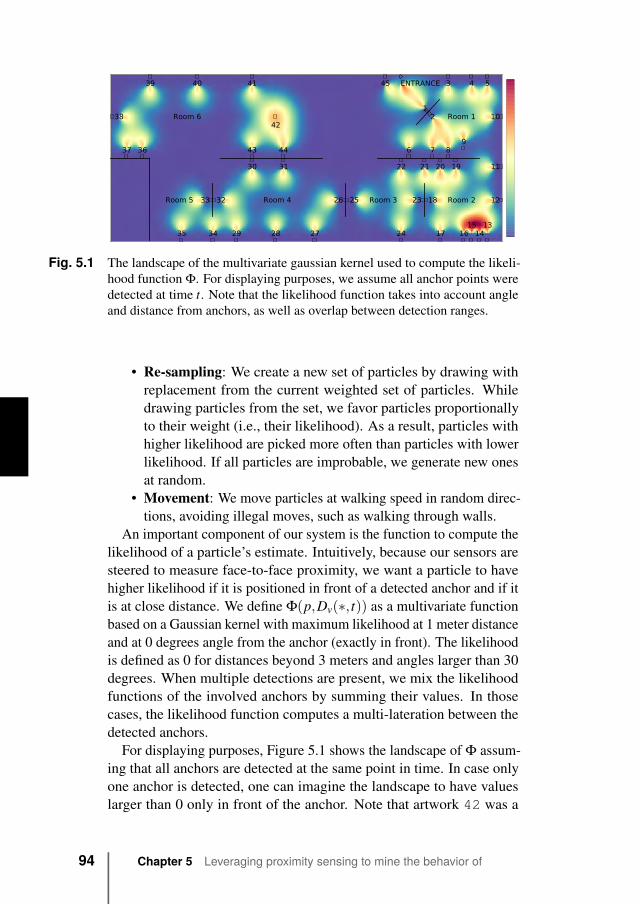
ENTRANCE

42

1315

Room 1

Room 2Room 3Room 4Room 5

Room 61

2

3 4 5

6 7 89

10

11

12

141617

18

19202122

23

24

2526

272829

30 31

3233

3435

3637

38

39 40 41

43 44

45

0.0

0.2

0.4

0.6

0.8

1.0

1.2

1.4

Fig. 5.1 The landscape of the multivariate gaussian kernel used to compute the likeli-hood function Φ. For displaying purposes, we assume all anchor points weredetected at time t. Note that the likelihood function takes into account angleand distance from anchors, as well as overlap between detection ranges.

• Re-sampling: We create a new set of particles by drawing withreplacement from the current weighted set of particles. Whiledrawing particles from the set, we favor particles proportionallyto their weight (i.e., their likelihood). As a result, particles withhigher likelihood are picked more often than particles with lowerlikelihood. If all particles are improbable, we generate new onesat random.

• Movement: We move particles at walking speed in random direc-tions, avoiding illegal moves, such as walking through walls.

An important component of our system is the function to compute thelikelihood of a particle’s estimate. Intuitively, because our sensors aresteered to measure face-to-face proximity, we want a particle to havehigher likelihood if it is positioned in front of a detected anchor and if itis at close distance. We define Φ(p,Dv(∗, t)) as a multivariate functionbased on a Gaussian kernel with maximum likelihood at 1 meter distanceand at 0 degrees angle from the anchor (exactly in front). The likelihoodis defined as 0 for distances beyond 3 meters and angles larger than 30degrees. When multiple detections are present, we mix the likelihoodfunctions of the involved anchors by summing their values. In thosecases, the likelihood function computes a multi-lateration between thedetected anchors.

For displaying purposes, Figure 5.1 shows the landscape of Φ assum-ing that all anchors are detected at the same point in time. In case onlyone anchor is detected, one can imagine the landscape to have valueslarger than 0 only in front of the anchor. Note that artwork 42 was a


museum visitors

cage, positioned far from the walls, of which visitors could walk around.For this reason, we placed the sensor inside an enclosure that alloweddetections from any angle, still within the same distance as defined forthe other artworks. The function models directionality and range of bothmobile devices and anchors, leveraging the radio directionality due tothe enclosures.

The filter keeps positioning a visitor at the last exhibit during gaps ofmissing detections. As soon as particles spread too much due to theirrandom movements, the filter assumes the visitor is far from any exhibit.Similarly, spurious detections from anchors far away or at the other sideof a wall are ignored as it takes time for particles to reach them (e.g.without crossing walls), and hence for their likelihood to be affected bythose anchors.

5.4.3 Density-based filter

The particle filter computes the positionings of a visitor regardless ofmissing, wrong, and ambiguous detections. The resulting matrix Mv

contains for each anchor a series of bits that tells us whenever a visitorwas facing an anchor at a certain time. While smoothened by the particlefilter, the series in Mv can still present gaps, for example, during shortperiods where particle confidence was too low (wrongly, due to manymissed detections), or when a visitor was wrongly associated to a nearbyexhibit. Even though they are rare, we want to remove these artifacts byfurther smoothening Mv through a density-based filter. In principle, thedensity-based filter acts analogously to a low-pass filter implementedthrough a sliding window, but it is able to compute the optimal valuesfor the parameters corresponding to window size and threshold.

The density-based filter [98] (see Chapter 4) first analyses all the seriesin Mv to compute the k-nearest neighbors statistics for each positioning,and it then uses these statistics to automatically identify bursts of bitsthrough the density-based clustering algorithm DBSCAN [55]. Eachidentified cluster is effectively a period of time when the visitor wascontinuously facing an exhibit. Once clusters are identified, we can fillthe gaps within the clusters. Note that, at the same time, the clusteringalgorithm classifies positionings that are isolated and not part of anycluster as noise. The result is a new positioning matrix M′v that iseffectively a smoothened version of Mv.

Note that, differently from Mv, in M′v visitor v can be positionedat multiple anchor points for the same time t, as series are filtered

5.4 Model 95

independently. We solve this problem in the next, and last, step of thepipeline.

5.4.4 Majority-voting filterWe define a majority-voting filter to disambiguate those times in M′vwhen we position v at more than one anchor (i.e., those columns of M′vthat have more than one row with a value of 1). The majority-voting filterlooks at a window of duration of L seconds ahead of, and including, t todecide at which anchor to position v. The filter decides by choosing theanchor with the largest number of positionings in that window of time.Formally, we let N windows w j,L,ai = 〈M′(i, j),M′(i, j+1), . . . ,M′(i, j+L)〉 slide in parallel over the series (i.e., rows) in M′v, with 0≤ j < T −L.We break ties by picking the anchor chosen at the previous slide, or atrandom when no anchor was chosen at the previous slide (i.e., whenall windows contain all zeros). While we filter M′v we create a newpositioning matrix M′′v and a path sequence sv of anchor AIDs thatrepresents the order used to visit the exhibits. We consider v to havetransitioned to a new exhibit when the filter positions v at an anchordifferent from the previous.

To summarize, for each visitor v, the pipeline outputs (i) the position-ing matrix M′′v representing at which anchor v was positioned, if any, ateach time t, and (ii) the sequence sv of anchors AIDs that represents inwhich order v visited the exhibits. Note that not necessarily all anchorare present in sv and also that an anchor AID can appear multiple times,though not consequently, in sv. Finally, we can compute a vector rv

of length N, that represents the number of seconds spent by the visitorfacing each exhibit. More precisely, we compute the values of rv asrv[i] = ∑

Tt=0 M′′v (i, t), for 0 < i < N. We will use rv and sv in Section 5.7

to identify group behavior.

5.5 Evaluation

5.5.1 MethodologyWe organized two experiments at CoBrA to evaluate our model andinfrastructure. In a controlled experiment, we scripted 28 visits andasked volunteers to follow the instructions through the script with atimer. The script defined a visit as a sequence of stops at exhibits, eachcharacterized by a time of arrival and a time of departure from eachexhibit. Volunteers were asked to stay at some 1-2 meters of distance


museum visitors

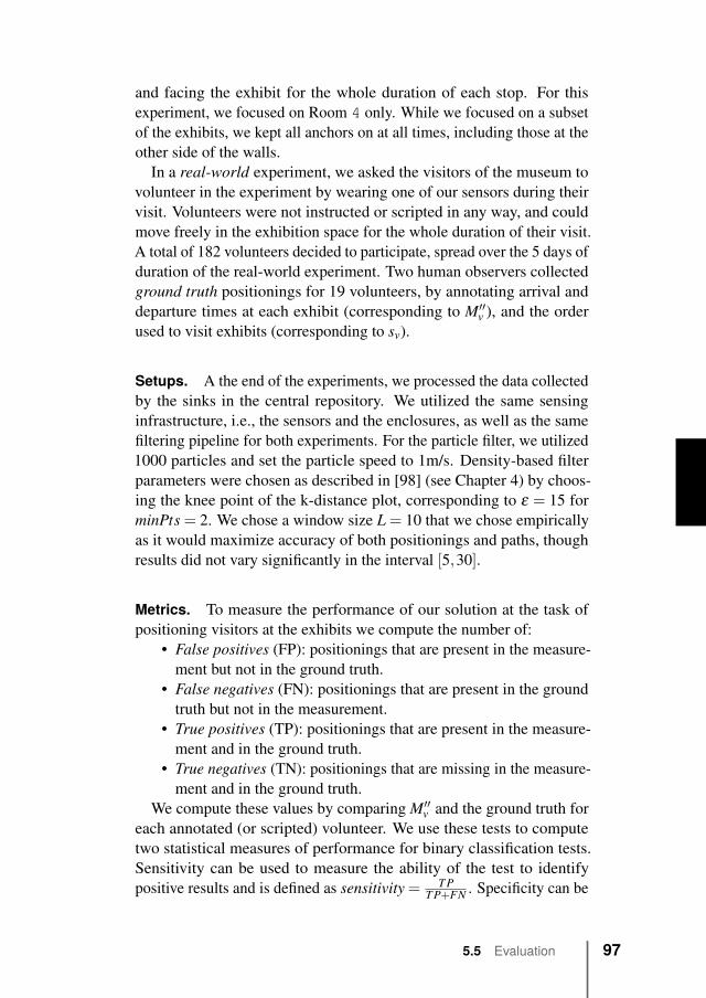
and facing the exhibit for the whole duration of each stop. For thisexperiment, we focused on Room 4 only. While we focused on a subsetof the exhibits, we kept all anchors on at all times, including those at theother side of the walls.

In a real-world experiment, we asked the visitors of the museum tovolunteer in the experiment by wearing one of our sensors during theirvisit. Volunteers were not instructed or scripted in any way, and couldmove freely in the exhibition space for the whole duration of their visit.A total of 182 volunteers decided to participate, spread over the 5 days ofduration of the real-world experiment. Two human observers collectedground truth positionings for 19 volunteers, by annotating arrival anddeparture times at each exhibit (corresponding to M′′v ), and the orderused to visit exhibits (corresponding to sv).

Setups. A the end of the experiments, we processed the data collectedby the sinks in the central repository. We utilized the same sensinginfrastructure, i.e., the sensors and the enclosures, as well as the samefiltering pipeline for both experiments. For the particle filter, we utilized1000 particles and set the particle speed to 1m/s. Density-based filterparameters were chosen as described in [98] (see Chapter 4) by choos-ing the knee point of the k-distance plot, corresponding to ε = 15 forminPts = 2. We chose a window size L = 10 that we chose empiricallyas it would maximize accuracy of both positionings and paths, thoughresults did not vary significantly in the interval [5,30].

Metrics. To measure the performance of our solution at the task ofpositioning visitors at the exhibits we compute the number of:

• False positives (FP): positionings that are present in the measure-ment but not in the ground truth.

• False negatives (FN): positionings that are present in the groundtruth but not in the measurement.

• True positives (TP): positionings that are present in the measure-ment and in the ground truth.

• True negatives (TN): positionings that are missing in the measure-ment and in the ground truth.

We compute these values by comparing M′′v and the ground truth foreach annotated (or scripted) volunteer. We use these tests to computetwo statistical measures of performance for binary classification tests.Sensitivity can be used to measure the ability of the test to identifypositive results and is defined as sensitivity = T P

T P+FN . Specificity can be

5.5 Evaluation 97

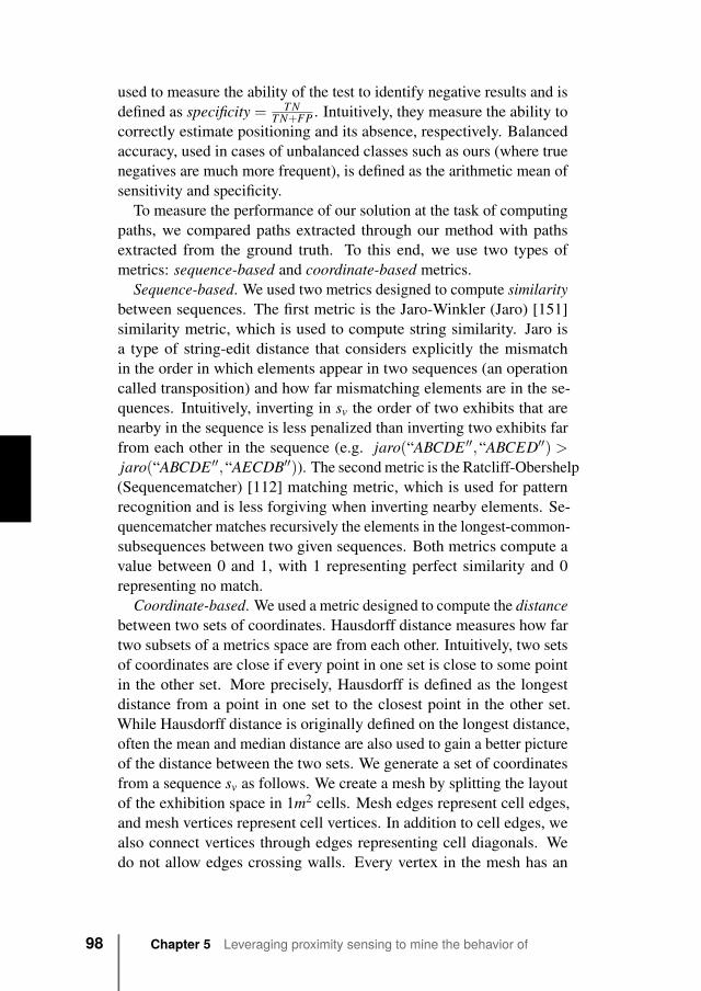
used to measure the ability of the test to identify negative results and isdefined as specificity = T N

T N+FP . Intuitively, they measure the ability tocorrectly estimate positioning and its absence, respectively. Balancedaccuracy, used in cases of unbalanced classes such as ours (where truenegatives are much more frequent), is defined as the arithmetic mean ofsensitivity and specificity.

To measure the performance of our solution at the task of computingpaths, we compared paths extracted through our method with pathsextracted from the ground truth. To this end, we use two types ofmetrics: sequence-based and coordinate-based metrics.

Sequence-based. We used two metrics designed to compute similaritybetween sequences. The first metric is the Jaro-Winkler (Jaro) [151]similarity metric, which is used to compute string similarity. Jaro isa type of string-edit distance that considers explicitly the mismatchin the order in which elements appear in two sequences (an operationcalled transposition) and how far mismatching elements are in the se-quences. Intuitively, inverting in sv the order of two exhibits that arenearby in the sequence is less penalized than inverting two exhibits farfrom each other in the sequence (e.g. jaro(“ABCDE ′′,“ABCED′′) >jaro(“ABCDE ′′,“AECDB′′)). The second metric is the Ratcliff-Obershelp(Sequencematcher) [112] matching metric, which is used for patternrecognition and is less forgiving when inverting nearby elements. Se-quencematcher matches recursively the elements in the longest-common-subsequences between two given sequences. Both metrics compute avalue between 0 and 1, with 1 representing perfect similarity and 0representing no match.

Coordinate-based. We used a metric designed to compute the distancebetween two sets of coordinates. Hausdorff distance measures how fartwo subsets of a metrics space are from each other. Intuitively, two setsof coordinates are close if every point in one set is close to some pointin the other set. More precisely, Hausdorff is defined as the longestdistance from a point in one set to the closest point in the other set.While Hausdorff distance is originally defined on the longest distance,often the mean and median distance are also used to gain a better pictureof the distance between the two sets. We generate a set of coordinatesfrom a sequence sv as follows. We create a mesh by splitting the layoutof the exhibition space in 1m2 cells. Mesh edges represent cell edges,and mesh vertices represent cell vertices. In addition to cell edges, wealso connect vertices through edges representing cell diagonals. Wedo not allow edges crossing walls. Every vertex in the mesh has an


museum visitors

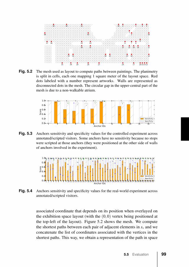
38

37 36

39

35

40

33

34

32

29

41

43

30

42

28

44

31

27

26 25

45 0

22

24

6

23

1

21

2

7

18

20

17

3

8

19

9

16

4

1514

5

13

10

11

12

Fig. 5.2 The mesh used as layout to compute paths between paintings. The planimetryis split in cells, each one mapping 1 square meter of the layout space. Reddots labeled with a number represent artworks. Walls are represented asdisconnected dots in the mesh. The circular gap in the upper-central part of themesh is due to a non-walkable atrium.

1 2 3 4 5 6 7 8 9 10 11 12Anchor IDs

0.0

0.2

0.4

0.6

0.8

1.0

Sco

re

Sensitivity

Specificity

Fig. 5.3 Anchors sensitivity and specificity values for the controlled experiment acrossannotated/scripted visitors. Some anchors have no sensitivity because no stopswere scripted at those anchors (they were positioned at the other side of wallsof anchors involved in the experiment).

1 2 3 4 5 6 7 8 9 10 11 12 13 14 15 16 17 18 19 20 21 22 23 24 25 26 27 28 29 30 31 32 33 34 36 37 38 39 40 41 42 43 44 45Anchor IDs

0.0

0.2

0.4

0.6

0.8

1.0

Sco

re

Sensitivity

Specificity

Fig. 5.4 Anchors sensitivity and specificity values for the real-world experiment acrossannotated/scripted visitors.

associated coordinate that depends on its position when overlayed onthe exhibition space layout (with the (0,0) vertex being positioned atthe top-left of the layout). Figure 5.2 shows the mesh. We computethe shortest paths between each pair of adjacent elements in sv and weconcatenate the list of coordinates associated with the vertices in theshortest paths. This way, we obtain a representation of the path in space

5.5 Evaluation 99

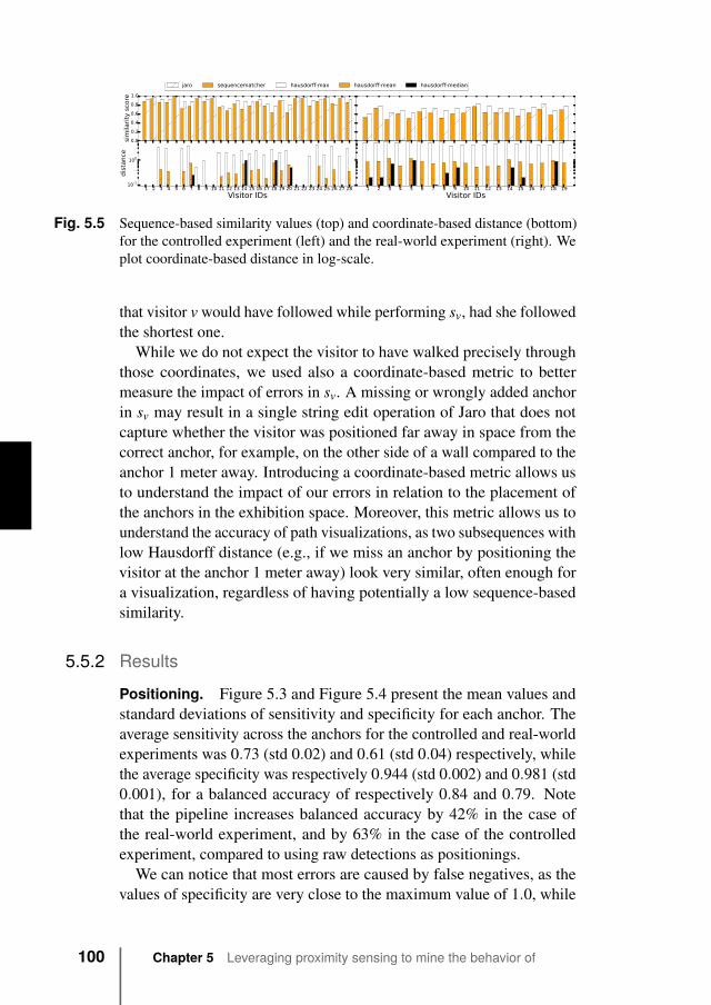
1 2 3 4 5 6 7 8 9 10 11 12 13 14 15 16 17 18 19 20 21 22 23 24 25 26 27 280.0

0.2

0.4

0.6

0.8

1.0

similarity score

1 2 3 4 5 6 7 8 9 10 11 12 13 14 15 16 17 18 19 20 21 22 23 24 25 26 27 28

Visitor IDs

10-1

100

distance

1 2 3 4 5 6 7 8 9 10 11 12 13 14 15 16 17 18 19

Visitor IDs

jaro sequencematcher hausdorff-max hausdorff-mean hausdorff-median

Fig. 5.5 Sequence-based similarity values (top) and coordinate-based distance (bottom)for the controlled experiment (left) and the real-world experiment (right). Weplot coordinate-based distance in log-scale.

that visitor v would have followed while performing sv, had she followedthe shortest one.

While we do not expect the visitor to have walked precisely throughthose coordinates, we used also a coordinate-based metric to bettermeasure the impact of errors in sv. A missing or wrongly added anchorin sv may result in a single string edit operation of Jaro that does notcapture whether the visitor was positioned far away in space from thecorrect anchor, for example, on the other side of a wall compared to theanchor 1 meter away. Introducing a coordinate-based metric allows usto understand the impact of our errors in relation to the placement ofthe anchors in the exhibition space. Moreover, this metric allows us tounderstand the accuracy of path visualizations, as two subsequences withlow Hausdorff distance (e.g., if we miss an anchor by positioning thevisitor at the anchor 1 meter away) look very similar, often enough fora visualization, regardless of having potentially a low sequence-basedsimilarity.

5.5.2 Results

Positioning. Figure 5.3 and Figure 5.4 present the mean values andstandard deviations of sensitivity and specificity for each anchor. Theaverage sensitivity across the anchors for the controlled and real-worldexperiments was 0.73 (std 0.02) and 0.61 (std 0.04) respectively, whilethe average specificity was respectively 0.944 (std 0.002) and 0.981 (std0.001), for a balanced accuracy of respectively 0.84 and 0.79. Notethat the pipeline increases balanced accuracy by 42% in the case ofthe real-world experiment, and by 63% in the case of the controlledexperiment, compared to using raw detections as positionings.

We can notice that most errors are caused by false negatives, as thevalues of specificity are very close to the maximum value of 1.0, while


museum visitors

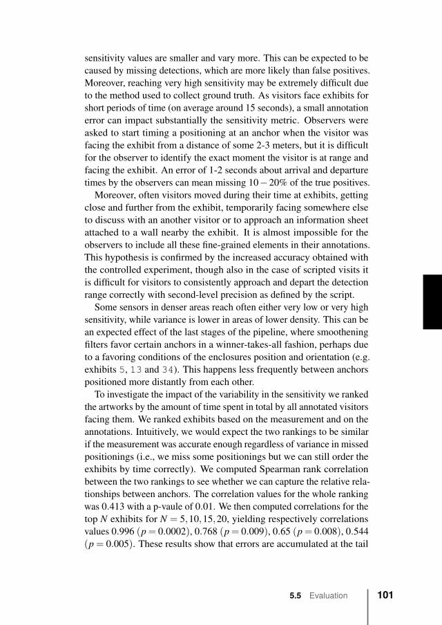
sensitivity values are smaller and vary more. This can be expected to becaused by missing detections, which are more likely than false positives.Moreover, reaching very high sensitivity may be extremely difficult dueto the method used to collect ground truth. As visitors face exhibits forshort periods of time (on average around 15 seconds), a small annotationerror can impact substantially the sensitivity metric. Observers wereasked to start timing a positioning at an anchor when the visitor wasfacing the exhibit from a distance of some 2-3 meters, but it is difficultfor the observer to identify the exact moment the visitor is at range andfacing the exhibit. An error of 1-2 seconds about arrival and departuretimes by the observers can mean missing 10−20% of the true positives.

Moreover, often visitors moved during their time at exhibits, gettingclose and further from the exhibit, temporarily facing somewhere elseto discuss with an another visitor or to approach an information sheetattached to a wall nearby the exhibit. It is almost impossible for theobservers to include all these fine-grained elements in their annotations.This hypothesis is confirmed by the increased accuracy obtained withthe controlled experiment, though also in the case of scripted visits itis difficult for visitors to consistently approach and depart the detectionrange correctly with second-level precision as defined by the script.

Some sensors in denser areas reach often either very low or very highsensitivity, while variance is lower in areas of lower density. This can bean expected effect of the last stages of the pipeline, where smootheningfilters favor certain anchors in a winner-takes-all fashion, perhaps dueto a favoring conditions of the enclosures position and orientation (e.g.exhibits 5, 13 and 34). This happens less frequently between anchorspositioned more distantly from each other.

To investigate the impact of the variability in the sensitivity we rankedthe artworks by the amount of time spent in total by all annotated visitorsfacing them. We ranked exhibits based on the measurement and on theannotations. Intuitively, we would expect the two rankings to be similarif the measurement was accurate enough regardless of variance in missedpositionings (i.e., we miss some positionings but we can still order theexhibits by time correctly). We computed Spearman rank correlationbetween the two rankings to see whether we can capture the relative rela-tionships between anchors. The correlation values for the whole rankingwas 0.413 with a p-vaule of 0.01. We then computed correlations for thetop N exhibits for N = 5,10,15,20, yielding respectively correlationsvalues 0.996 (p = 0.0002), 0.768 (p = 0.009), 0.65 (p = 0.008), 0.544(p = 0.005). These results show that errors are accumulated at the tail

5.5 Evaluation 101

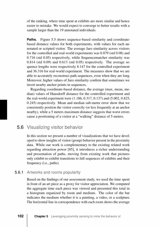
of the ranking, where time spent at exhibits are more similar and henceeasier to mistake. We would expect to converge to better results with asample larger than the 19 annotated individuals.

Paths. Figure 5.5 shows sequence-based similarity and coordinate-based distance values for both experiments, with values for each an-notated or scripted visitor. The average Jaro similarity across visitorsfor the controlled and real-world experiments was 0.879 (std 0.08) and0.716 (std 0.05) respectively, while Sequencematcher similarity was0.814 (std 0.09) and 0.613 (std 0.05) respectively. The average se-quence lengths were respectively 8.147 for the controlled experimentand 36.316 for real-world experiment. The measures show that we areable to accurately reconstruct path sequences, even when they are long.Moreover, higher values of Jaro similarity confirm that sometimes weinvert nearby anchor points in sequences.

Regarding coordinate-based distance, the average (max, mean, me-dian) values of Hausdorff distance for the controlled experiment andthe real-world experiment were (1.186, 0.317, 0.137) and (5.002, 0.825,0.245) respectively. Mean and median sub-meter error show that weconsistently position the visitor correctly (or less frequently at an anchornearby), while a 5 meters maximum distance suggests that worst errorscause a positioning of a visitor at a “walking” distance of 5 meters.

5.6 Visualizing visitor behaviorIn this section we present a number of visualizations that we have devel-oped to show insights of visitor (group) behavior present in the proximitydata. While our work is complementary to the existing related workregarding attraction power [85], it introduces a richer understandingand presentation of paths, moving from existing work that picturesonly exhibit-to-exhibit transitions to full sequences of exhibits and theirfrequency (i.e., paths).

5.6.1 Artworks and rooms popularityBased on the findings of our assessment study, we used the time spentin front of an art piece as a proxy for visitor appreciation. We computedthe aggregate time each piece was viewed and presented this total ina histogram organized by room and medium. The color of the barindicates the medium whether it is a painting, a video, or a sculpture.The horizontal line in correspondence with each room shows the average


museum visitors

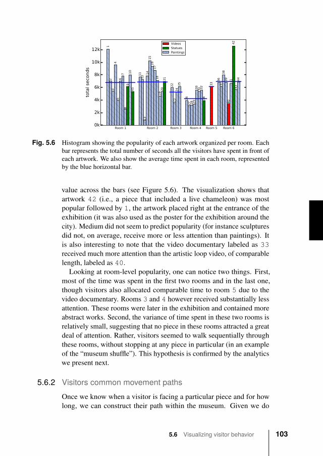
0k

2k

4k

6k

8k

10k

12k

total seconds

12

34

56

78

910

45

Room 1

11

12

13

14

15

16

17

18

1920

21

Room 2

22

23

24

25

Room 3

26

27 28 29

30

31 32

34

Room 4

33

Room 5

36

37

38

39

40

41

42

43

44

Room 6

Videos

Statues

Paintings

Fig. 5.6 Histogram showing the popularity of each artwork organized per room. Eachbar represents the total number of seconds all the visitors have spent in front ofeach artwork. We also show the average time spent in each room, representedby the blue horizontal bar.

value across the bars (see Figure 5.6). The visualization shows thatartwork 42 (i.e., a piece that included a live chameleon) was mostpopular followed by 1, the artwork placed right at the entrance of theexhibition (it was also used as the poster for the exhibition around thecity). Medium did not seem to predict popularity (for instance sculpturesdid not, on average, receive more or less attention than paintings). Itis also interesting to note that the video documentary labeled as 33received much more attention than the artistic loop video, of comparablelength, labeled as 40.

Looking at room-level popularity, one can notice two things. First,most of the time was spent in the first two rooms and in the last one,though visitors also allocated comparable time to room 5 due to thevideo documentary. Rooms 3 and 4 however received substantially lessattention. These rooms were later in the exhibition and contained moreabstract works. Second, the variance of time spent in these two rooms isrelatively small, suggesting that no piece in these rooms attracted a greatdeal of attention. Rather, visitors seemed to walk sequentially throughthese rooms, without stopping at any piece in particular (in an exampleof the “museum shuffle”). This hypothesis is confirmed by the analyticswe present next.

5.6.2 Visitors common movement pathsOnce we know when a visitor is facing a particular piece and for howlong, we can construct their path within the museum. Given we do

5.6 Visualizing visitor behavior 103

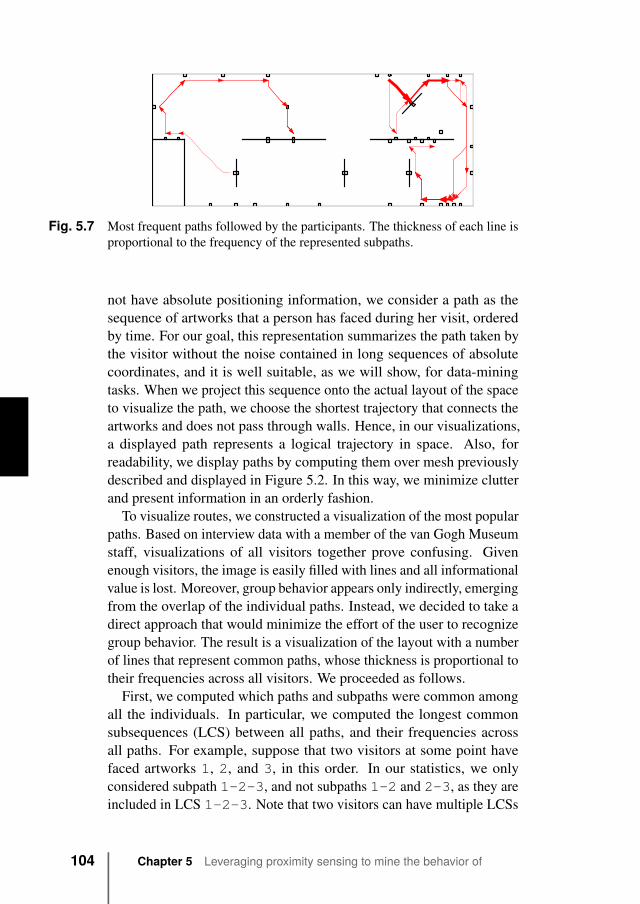
Fig. 5.7 Most frequent paths followed by the participants. The thickness of each line isproportional to the frequency of the represented subpaths.

not have absolute positioning information, we consider a path as thesequence of artworks that a person has faced during her visit, orderedby time. For our goal, this representation summarizes the path taken bythe visitor without the noise contained in long sequences of absolutecoordinates, and it is well suitable, as we will show, for data-miningtasks. When we project this sequence onto the actual layout of the spaceto visualize the path, we choose the shortest trajectory that connects theartworks and does not pass through walls. Hence, in our visualizations,a displayed path represents a logical trajectory in space. Also, forreadability, we display paths by computing them over mesh previouslydescribed and displayed in Figure 5.2. In this way, we minimize clutterand present information in an orderly fashion.

To visualize routes, we constructed a visualization of the most popularpaths. Based on interview data with a member of the van Gogh Museumstaff, visualizations of all visitors together prove confusing. Givenenough visitors, the image is easily filled with lines and all informationalvalue is lost. Moreover, group behavior appears only indirectly, emergingfrom the overlap of the individual paths. Instead, we decided to take adirect approach that would minimize the effort of the user to recognizegroup behavior. The result is a visualization of the layout with a numberof lines that represent common paths, whose thickness is proportional totheir frequencies across all visitors. We proceeded as follows.

First, we computed which paths and subpaths were common amongall the individuals. In particular, we computed the longest commonsubsequences (LCS) between all paths, and their frequencies acrossall paths. For example, suppose that two visitors at some point havefaced artworks 1, 2, and 3, in this order. In our statistics, we onlyconsidered subpath 1-2-3, and not subpaths 1-2 and 2-3, as they areincluded in LCS 1-2-3. Note that two visitors can have multiple LCSs


museum visitors

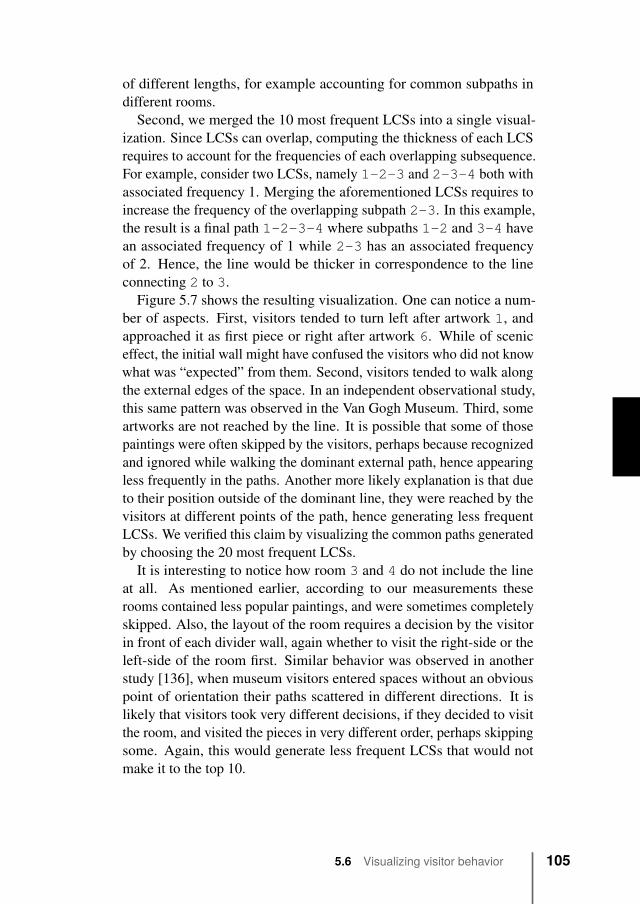
of different lengths, for example accounting for common subpaths indifferent rooms.

Second, we merged the 10 most frequent LCSs into a single visual-ization. Since LCSs can overlap, computing the thickness of each LCSrequires to account for the frequencies of each overlapping subsequence.For example, consider two LCSs, namely 1-2-3 and 2-3-4 both withassociated frequency 1. Merging the aforementioned LCSs requires toincrease the frequency of the overlapping subpath 2-3. In this example,the result is a final path 1-2-3-4 where subpaths 1-2 and 3-4 havean associated frequency of 1 while 2-3 has an associated frequencyof 2. Hence, the line would be thicker in correspondence to the lineconnecting 2 to 3.

Figure 5.7 shows the resulting visualization. One can notice a num-ber of aspects. First, visitors tended to turn left after artwork 1, andapproached it as first piece or right after artwork 6. While of sceniceffect, the initial wall might have confused the visitors who did not knowwhat was “expected” from them. Second, visitors tended to walk alongthe external edges of the space. In an independent observational study,this same pattern was observed in the Van Gogh Museum. Third, someartworks are not reached by the line. It is possible that some of thosepaintings were often skipped by the visitors, perhaps because recognizedand ignored while walking the dominant external path, hence appearingless frequently in the paths. Another more likely explanation is that dueto their position outside of the dominant line, they were reached by thevisitors at different points of the path, hence generating less frequentLCSs. We verified this claim by visualizing the common paths generatedby choosing the 20 most frequent LCSs.

It is interesting to notice how room 3 and 4 do not include the lineat all. As mentioned earlier, according to our measurements theserooms contained less popular paintings, and were sometimes completelyskipped. Also, the layout of the room requires a decision by the visitorin front of each divider wall, again whether to visit the right-side or theleft-side of the room first. Similar behavior was observed in anotherstudy [136], when museum visitors entered spaces without an obviouspoint of orientation their paths scattered in different directions. It islikely that visitors took very different decisions, if they decided to visitthe room, and visited the pieces in very different order, perhaps skippingsome. Again, this would generate less frequent LCSs that would notmake it to the top 10.


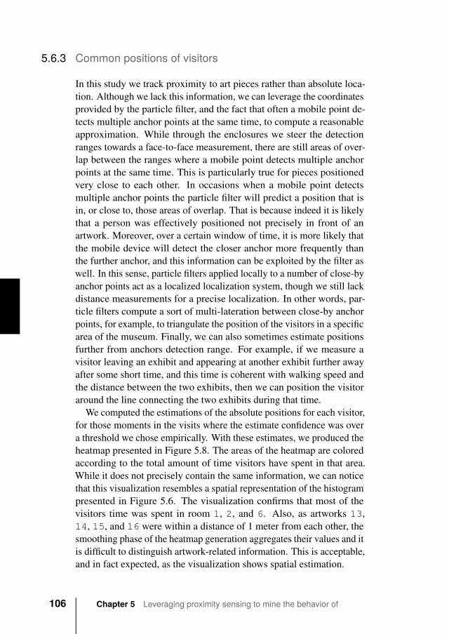
5.6.3 Common positions of visitors

In this study we track proximity to art pieces rather than absolute loca-tion. Although we lack this information, we can leverage the coordinatesprovided by the particle filter, and the fact that often a mobile point de-tects multiple anchor points at the same time, to compute a reasonableapproximation. While through the enclosures we steer the detectionranges towards a face-to-face measurement, there are still areas of over-lap between the ranges where a mobile point detects multiple anchorpoints at the same time. This is particularly true for pieces positionedvery close to each other. In occasions when a mobile point detectsmultiple anchor points the particle filter will predict a position that isin, or close to, those areas of overlap. That is because indeed it is likelythat a person was effectively positioned not precisely in front of anartwork. Moreover, over a certain window of time, it is more likely thatthe mobile device will detect the closer anchor more frequently thanthe further anchor, and this information can be exploited by the filter aswell. In this sense, particle filters applied locally to a number of close-byanchor points act as a localized localization system, though we still lackdistance measurements for a precise localization. In other words, par-ticle filters compute a sort of multi-lateration between close-by anchorpoints, for example, to triangulate the position of the visitors in a specificarea of the museum. Finally, we can also sometimes estimate positionsfurther from anchors detection range. For example, if we measure avisitor leaving an exhibit and appearing at another exhibit further awayafter some short time, and this time is coherent with walking speed andthe distance between the two exhibits, then we can position the visitoraround the line connecting the two exhibits during that time.

We computed the estimations of the absolute positions for each visitor,for those moments in the visits where the estimate confidence was overa threshold we chose empirically. With these estimates, we produced theheatmap presented in Figure 5.8. The areas of the heatmap are coloredaccording to the total amount of time visitors have spent in that area.While it does not precisely contain the same information, we can noticethat this visualization resembles a spatial representation of the histogrampresented in Figure 5.6. The visualization confirms that most of thevisitors time was spent in room 1, 2, and 6. Also, as artworks 13,14, 15, and 16 were within a distance of 1 meter from each other, thesmoothing phase of the heatmap generation aggregates their values and itis difficult to distinguish artwork-related information. This is acceptable,and in fact expected, as the visualization shows spatial estimation.


museum visitors

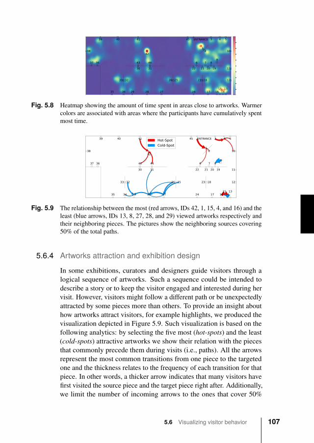
ENTRANCE

42

1315

12

3 4 5

6 7 89

10

11

12

141617

18

19202122

23

24

2526

272829

30 31

3233

3435

3637

38

39 40 41

43 44

45

0

8

16

24

32

40

48

56

64

72

Fig. 5.8 Heatmap showing the amount of time spent in areas close to artworks. Warmercolors are associated with areas where the participants have cumulatively spentmost time.

ENTRANCE

42

1315

12

3 4 5

6 7 89

10

11

12

141617

18

19202122

23

24

2526

272829

30 31

3233

3435

3637

38

39 40 41

43 44

45Hot-Spot

Cold-Spot

Fig. 5.9 The relationship between the most (red arrows, IDs 42, 1, 15, 4, and 16) and theleast (blue arrows, IDs 13, 8, 27, 28, and 29) viewed artworks respectively andtheir neighboring pieces. The pictures show the neighboring sources covering50% of the total paths.

5.6.4 Artworks attraction and exhibition design

In some exhibitions, curators and designers guide visitors through alogical sequence of artworks. Such a sequence could be intended todescribe a story or to keep the visitor engaged and interested during hervisit. However, visitors might follow a different path or be unexpectedlyattracted by some pieces more than others. To provide an insight abouthow artworks attract visitors, for example highlights, we produced thevisualization depicted in Figure 5.9. Such visualization is based on thefollowing analytics: by selecting the five most (hot-spots) and the least(cold-spots) attractive artworks we show their relation with the piecesthat commonly precede them during visits (i.e., paths). All the arrowsrepresent the most common transitions from one piece to the targetedone and the thickness relates to the frequency of each transition for thatpiece. In other words, a thicker arrow indicates that many visitors havefirst visited the source piece and the target piece right after. Additionally,we limit the number of incoming arrows to the ones that cover 50%


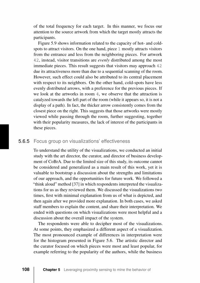
of the total frequency for each target. In this manner, we focus ourattention to the source artwork from which the target mostly attracts theparticipants.

Figure 5.9 shows information related to the capacity of hot- and cold-spots to attract visitors. On the one hand, piece 1 mostly attracts visitorsfrom the entrance and less from the neighboring pieces. For artwork42, instead, visitor transitions are evenly distributed among the mostimmediate pieces. This result suggests that visitors may approach 42due its attractiveness more than due to a sequential scanning of the room.However, such effect could also be attributed to its central placementwith respect to its neighbors. On the other hand, cold-spots have lessevenly distributed arrows, with a preference for the previous pieces. Ifwe look at the artworks in room 4, we observe that the attraction iscatalyzed towards the left part of the room (while it appears so, it is not adisplay of a path). In fact, the thicker arrow consistently comes from theclosest piece on the right. This suggests that those artworks were mostlyviewed while passing through the room, further suggesting, togetherwith their popularity measures, the lack of interest of the participants inthese pieces.

5.6.5 Focus group on visualizations’ effectivenessTo understand the utility of the visualizations, we conducted an initialstudy with the art director, the curator, and director of business develop-ment of CoBrA. Due to the limited size of this study, its outcome cannotbe considered and generalized as a main result of this work, yet it isvaluable to bootstrap a discussion about the strengths and limitationsof our approach, and the opportunities for future work. We followed a“think aloud” method [37] in which respondents interpreted the visualiza-tions for us as they reviewed them. We discussed the visualizations twotimes, first with minimal explanation from us of what is depicted, andthen again after we provided more explanation. In both cases, we askedstaff members to explain the content, and share their interpretation. Weended with questions on which visualizations were most helpful and adiscussion about the overall impact of the system.

The respondents were able to decipher most of the visualizations.At some points, they emphasized a different aspect of a visualization.The most pronounced example of differences in interpretation werefor the histogram presented in Figure 5.6. The artistic director andthe curator focused on which pieces were most and least popular, forexample referring to the popularity of the authors, while the business


museum visitors

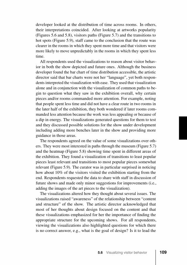
developer looked at the distribution of time across rooms. In others,their interpretations coincided. After looking at artworks popularity(Figures 5.6 and 5.8), visitors paths (Figure 5.7) and the transitions tohot spots (Figure 5.9), staff came to the conclusion that the route wasclearer in the rooms in which they spent more time and that visitors weremore likely to move unpredictably in the rooms in which they spent lesstime.

All respondents used the visualizations to reason about visitor behav-ior in both the show depicted and future ones. Although the businessdeveloper found the bar chart of time distribution accessible, the artisticdirector said that bar charts were not her “language”, yet both respon-dents interpreted the visualization with ease. They used that visualizationalone and in conjunction with the visualization of common paths to be-gin to question what they saw in the exhibition overall, why certainpieces and/or rooms commanded more attention. For example, notingthat people spent less time and did not have a clear route in two rooms inthe later half of the exhibition, they both wondered if later rooms com-manded less attention because the work was less appealing or because ofa dip in energy. The visualizations generated questions for them to testand they discussed possible solutions for the show under developmentincluding adding more benches later in the show and providing moreguidance in those areas.

The respondents agreed on the value of some visualizations over oth-ers. They were most interested in paths through the museum (Figure 5.7)and the heatmap (Figure 5.8) showing time spent in different areas ofthe exhibition. They found a visualization of transitions to least popularpieces least relevant and transitions to most popular pieces somewhatrelevant (Figure 5.9). The curator was in particular surprised in noticinghow about 10% of the visitors visited the exhibition starting from theend. Respondents requested the data to share with staff in discussion offuture shows and made only minor suggestions for improvements (i.e.,adding the images of the art pieces to the visualization).

The visualizations altered how they thought about several issues. Thevisualizations raised “awareness” of the relationship between “contentand structure” of the show. The artistic director acknowledged thatmost of her thoughts about design focused on the content and thatthese visualizations emphasized for her the importance of finding theappropriate structure for the upcoming shows. For all respondents,viewing the visualizations also highlighted questions for which thereis no correct answer, e.g., what is the goal of design? Is it to lead the


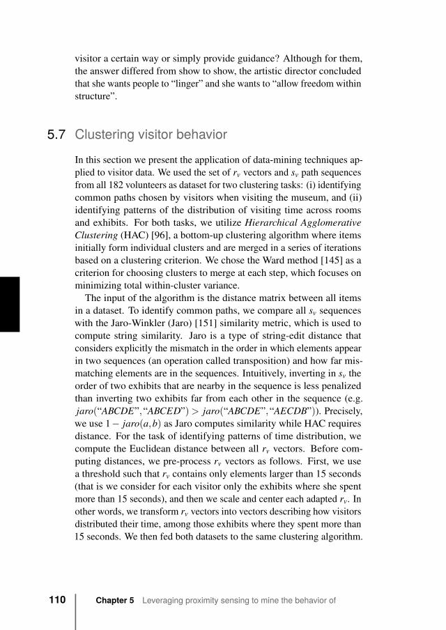
visitor a certain way or simply provide guidance? Although for them,the answer differed from show to show, the artistic director concludedthat she wants people to “linger” and she wants to “allow freedom withinstructure”.

5.7 Clustering visitor behavior

In this section we present the application of data-mining techniques ap-plied to visitor data. We used the set of rv vectors and sv path sequencesfrom all 182 volunteers as dataset for two clustering tasks: (i) identifyingcommon paths chosen by visitors when visiting the museum, and (ii)identifying patterns of the distribution of visiting time across roomsand exhibits. For both tasks, we utilize Hierarchical AgglomerativeClustering (HAC) [96], a bottom-up clustering algorithm where itemsinitially form individual clusters and are merged in a series of iterationsbased on a clustering criterion. We chose the Ward method [145] as acriterion for choosing clusters to merge at each step, which focuses onminimizing total within-cluster variance.

The input of the algorithm is the distance matrix between all itemsin a dataset. To identify common paths, we compare all sv sequenceswith the Jaro-Winkler (Jaro) [151] similarity metric, which is used tocompute string similarity. Jaro is a type of string-edit distance thatconsiders explicitly the mismatch in the order in which elements appearin two sequences (an operation called transposition) and how far mis-matching elements are in the sequences. Intuitively, inverting in sv theorder of two exhibits that are nearby in the sequence is less penalizedthan inverting two exhibits far from each other in the sequence (e.g.jaro(“ABCDE”,“ABCED”)> jaro(“ABCDE”,“AECDB”)). Precisely,we use 1− jaro(a,b) as Jaro computes similarity while HAC requiresdistance. For the task of identifying patterns of time distribution, wecompute the Euclidean distance between all rv vectors. Before com-puting distances, we pre-process rv vectors as follows. First, we usea threshold such that rv contains only elements larger than 15 seconds(that is we consider for each visitor only the exhibits where she spentmore than 15 seconds), and then we scale and center each adapted rv. Inother words, we transform rv vectors into vectors describing how visitorsdistributed their time, among those exhibits where they spent more than15 seconds. We then fed both datasets to the same clustering algorithm.


museum visitors

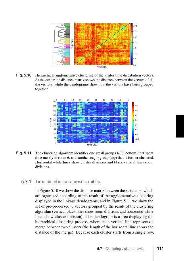
visitors

vis

itors

0.0

1.5

3.0

4.5

6.0

7.5

9.0

10.5

Fig. 5.10 Hierarchical agglomerative clustering of the visitor time distribution vectors.At the center the distance matrix shows the distance between the vectors of allthe visitors, while the dendograms show how the visitors have been groupedtogether.

0 5 10 15 20 25 30 35 40 45

exhibits0

20

40

60

80

100

120

140

160

180

vis

itors

0.8

0.0

0.8

1.6

2.4

3.2

4.0

4.8

Fig. 5.11 The clustering algorithm identifies one small group (1-38, bottom) that spenttime mostly in room 6, and another major group (top) that is further clustered.Horizontal white lines show cluster divisions and black vertical lines roomdivisions.

5.7.1 Time distribution across exhibits

In Figure 5.10 we show the distance matrix between the rv vectors, whichare organized according to the result of the agglomerative clusteringdisplayed in the linkage dendograms, and in Figure 5.11 we show theset of pre-processed rv vectors grouped by the result of the clusteringalgorithm (vertical black lines show room divisions and horizontal whitelines show cluster division). The dendogram is a tree displaying thehierarchical clustering process, where each vertical line represents amerge between two clusters (the length of the horizontal line shows thedistance of the merge). Because each cluster starts from a single row,

5.7 Clustering visitor behavior 111

one can notice that each merge starts by merging two rows togetherup to the root. The distance matrix shows the distance between eachvisitor. One can notice that distance between visitors in the same clusteris lower than between visitors between visitors belonging to differentclusters. Because the visitors are organized according to the results ofhierarchical clustering, the distance matrix can give an intuition of theboundaries of the clusters that are merged at each step.

The results show that the clustering algorithm identifies two majorclusters. The first cluster includes the bottom visitors (1-38, light greenand red in the dendogram) for their particular interest in 3 artworks inroom 6 and little interest in room 2 and 3 except for exhibit 1. Thesecond cluster includes all visitors between (65-182) who spent timein room 2 and in front of exhibit 42. This second cluster is furtherclustered in other clusters, for example, (i) (85-118, yellow) due tospecific interest in the exhibits 7, 8, 9, (ii) (124-160, black) due tospecific interest in the first three exhibits, (iii) (160-182, green) due tosome specific interest in exhibits 38, 39, 40 and 41, as well as 19, 20,and 21. Finally, HAC puts all outliers in a cluster together (38-65, lightblue), though some of them do show a pattern, as it is the case of 40-50,showing a common interest in exhibits 2, 3, 4, as well as 14, 15, and38 and 39.

5.7.2 Clustering of pathsWe applied the same technique to paths. In Figure 5.12 and Figure 5.13we show two of the clusters identified with HAC. We constructed thevisualization as described previously, but focusing only on each chosencluster, and this time selecting the most frequent 20 LCSs.

The first cluster includes the largest group of visitors and shows themost common behavior. HAC identified further groups within this majorcluster, for example, splitting visitors turning right towards exhibit 6from visitors turning left towards exhibit 3 after exhibit 1 at the entrance.The second cluster in Figure 5.13 shows a cluster with 10% of the visitorswho visited the exhibition space in “inverted order”, starting from room6. Perhaps these visitors did not understand what was expected fromthem by the curators. Similarly, through HAC we identified anothergroup of visitors who decided to visit room 6 first, only to return rightback to room 1 and continued from there, perhaps after realizing theirmistake.

Furthermore, we can notice that both groups make more differentchoices of paths while visiting the first rooms, whereas the last rooms


museum visitors

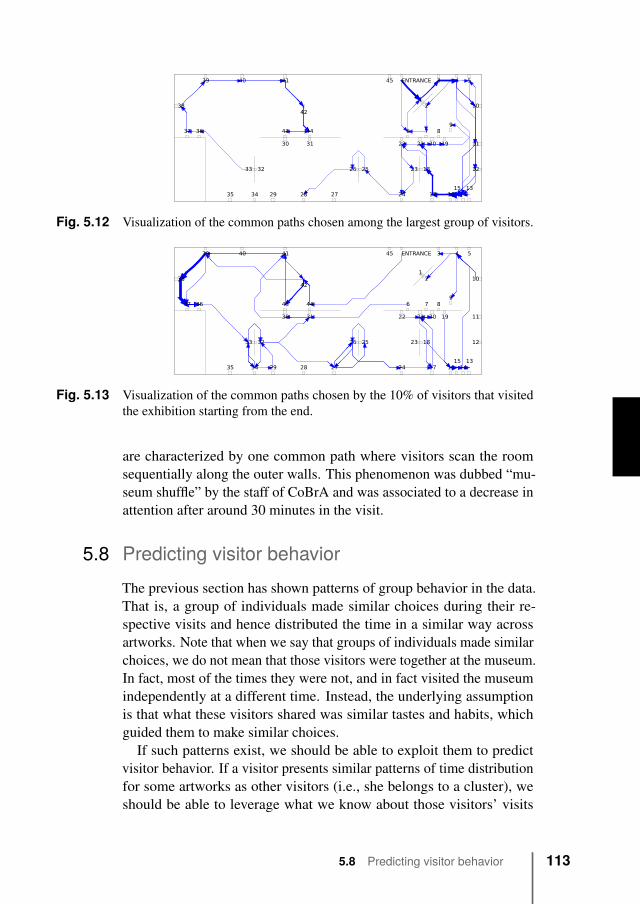
ENTRANCE

42

1315

12

3 4 5

6 7 89

10

11

12

141617

18

19202122

23

24

2526

272829

30 31

3233

3435

3637

38

39 40 41

43 44

45

Fig. 5.12 Visualization of the common paths chosen among the largest group of visitors.

ENTRANCE

42

1315

12

3 4 5

6 7 89

10

11

12

141617

18

19202122

23

24

2526

272829

30 31

3233

3435

3637

38

39 40 41

43 44

45

Fig. 5.13 Visualization of the common paths chosen by the 10% of visitors that visitedthe exhibition starting from the end.

are characterized by one common path where visitors scan the roomsequentially along the outer walls. This phenomenon was dubbed “mu-seum shuffle” by the staff of CoBrA and was associated to a decrease inattention after around 30 minutes in the visit.

5.8 Predicting visitor behaviorThe previous section has shown patterns of group behavior in the data.That is, a group of individuals made similar choices during their re-spective visits and hence distributed the time in a similar way acrossartworks. Note that when we say that groups of individuals made similarchoices, we do not mean that those visitors were together at the museum.In fact, most of the times they were not, and in fact visited the museumindependently at a different time. Instead, the underlying assumptionis that what these visitors shared was similar tastes and habits, whichguided them to make similar choices.

If such patterns exist, we should be able to exploit them to predictvisitor behavior. If a visitor presents similar patterns of time distributionfor some artworks as other visitors (i.e., she belongs to a cluster), weshould be able to leverage what we know about those visitors’ visits

5.8 Predicting visitor behavior 113

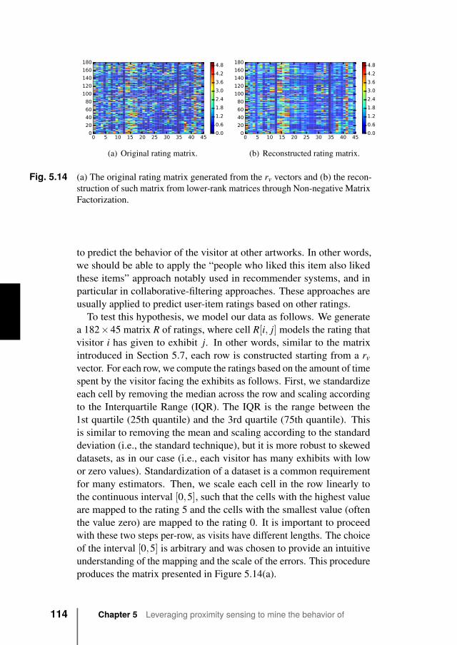
0 5 10 15 20 25 30 35 40 450

20

40

60

80

100

120

140

160

180

0.0

0.6

1.2

1.8

2.4

3.0

3.6

4.2

4.8

(a) Original rating matrix.

0 5 10 15 20 25 30 35 40 450

20

40

60

80

100

120

140

160

180

0.0

0.6

1.2

1.8

2.4

3.0

3.6

4.2

4.8

(b) Reconstructed rating matrix.

Fig. 5.14 (a) The original rating matrix generated from the rv vectors and (b) the recon-struction of such matrix from lower-rank matrices through Non-negative MatrixFactorization.

to predict the behavior of the visitor at other artworks. In other words,we should be able to apply the “people who liked this item also likedthese items” approach notably used in recommender systems, and inparticular in collaborative-filtering approaches. These approaches areusually applied to predict user-item ratings based on other ratings.

To test this hypothesis, we model our data as follows. We generatea 182×45 matrix R of ratings, where cell R[i, j] models the rating thatvisitor i has given to exhibit j. In other words, similar to the matrixintroduced in Section 5.7, each row is constructed starting from a rv

vector. For each row, we compute the ratings based on the amount of timespent by the visitor facing the exhibits as follows. First, we standardizeeach cell by removing the median across the row and scaling accordingto the Interquartile Range (IQR). The IQR is the range between the1st quartile (25th quantile) and the 3rd quartile (75th quantile). Thisis similar to removing the mean and scaling according to the standarddeviation (i.e., the standard technique), but it is more robust to skeweddatasets, as in our case (i.e., each visitor has many exhibits with lowor zero values). Standardization of a dataset is a common requirementfor many estimators. Then, we scale each cell in the row linearly tothe continuous interval [0,5], such that the cells with the highest valueare mapped to the rating 5 and the cells with the smallest value (oftenthe value zero) are mapped to the rating 0. It is important to proceedwith these two steps per-row, as visits have different lengths. The choiceof the interval [0,5] is arbitrary and was chosen to provide an intuitiveunderstanding of the mapping and the scale of the errors. This procedureproduces the matrix presented in Figure 5.14(a).


museum visitors

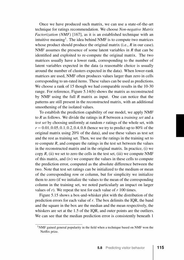
Once we have produced such matrix, we can use a state-of-the-arttechnique for ratings recommendation. We choose Non-negative MatrixFactorization (NMF) [167], as it is an established technique with anintuitive meaning1. The idea behind NMF is to compute two matriceswhose product should produce the original matrix (i.e., R in our case).NMF assumes the presence of some latent variables in R that can beidentified and exploited to re-compute the original matrix. The twomatrices usually have a lower rank, corresponding to the number oflatent variables expected in the data (a reasonable choice is usuallyaround the number of clusters expected in the data). When lower-rankmatrices are used, NMF often produces values larger than zero in cellscorresponding to un-rated items. These values can be used as predictions.We choose a rank of 15 though we had comparable results in the 10-30range. For reference, Figure 5.14(b) shows the matrix as reconstructedby NMF using the full R matrix as input. One can notice that thepatterns are still present in the reconstructed matrix, with an additionalsmoothening of the isolated values.

To establish the prediction capability of our model, we apply NMFto R as follows. We divide the ratings in R between a training set and atest set by choosing uniformly at random r ratings of the whole set, withr = 0.01,0.05,0.1,0.2,0.4,0.8 (hence we try to predict up to 80% of theoriginal matrix using 20% of the data), and use these values as test setand the rest as training set. Then, we use the ratings in the training set tore-compute R, and compare the ratings in the test set between the valuesin the reconstructed matrix and in the original matrix. In practice, (i) wecopy R, (ii) we set to zero the cells in the test set, (iii) we compute NMFof this matrix, and (iv) we compare the values in these cells to computethe prediction error, computed as the absolute difference between thetwo. Note that test set ratings can be initialized to the medium or meanof the corresponding row or column, but for simplicity we initializethem to zero (if we initialize the values to the mean of the correspondingcolumn in the training set, we noted particularly an impact on largervalues of r). We repeat the test for each value of r 100 times.

Figure 5.15 shows a box-and-whisker plot with the distribution of theprediction errors for each value of r. The box delimits the IQR, the bandand the square in the box are the median and the mean respectively, thewhiskers are set at the 1.5 of the IQR, and outer points are the outliers.We can see that the median prediction error is consistently beneath 1

1NMF gained general popularity in the field when a technique based on NMF won theNetflix prize.

5.8 Predicting visitor behavior 115

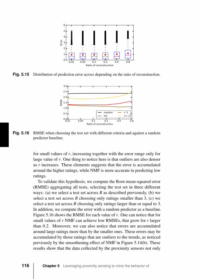
0.01 0.05 0.1 0.2 0.4 0.8Ratio of reconstruction

0

1

2

3

4

5

6

Error

Fig. 5.15 Distribution of prediction error across depending on the ratio of reconstruction.

0.01 0.05 0.1 0.2 0.4 0.8Ratio of reconstruction

0.0

0.5

1.0

1.5

2.0

2.5

3.0

RMSE

random

full

< 3

>= 3

Fig. 5.16 RMSE when choosing the test set with different criteria and against a randompredictor baseline.

for small values of r, increasing together with the error range only forlarge value of r. One thing to notice here is that outliers are also denseras r increases. These elements suggests that the error is accumulatedaround the higher ratings, while NMF is more accurate in predicting lowratings.

To validate this hypothesis, we compute the Root-mean-squared error(RMSE) aggregating all tests, selecting the test set in three differentways: (a) we select a test set across R as described previously, (b) weselect a test set across R choosing only ratings smaller than 3, (c) weselect a test set across R choosing only ratings larger than or equal to 3.In addition, we compute the error with a random predictor as a baseline.Figure 5.16 shows the RMSE for each value of r. One can notice that forsmall values of r NMF can achieve low RMSEs, that grow for r largerthan 0.2. Moreover, we can also notice that errors are accumulatedaround large ratings more than by the smaller ones. These errors may beaccumulated by those ratings that are outliers to the trends, as noticedpreviously by the smoothening effect of NMF in Figure 5.14(b). Theseresults show that the data collected by the proximity sensors not only


museum visitors

show group behavior, but that can also be used to predict the behavior ofthe visitors. Note that in terms of pure RMSE, we obtained lower errorswhen initializing the test set cells to the mean value of the column (i.e.,around 1.6 for r = 0.01), but minimizing the RMSE is out of scope ofthis work.

5.9 Discussion

The proposed solution is able to reconstruct the behavior of a groupof visitors with a pipeline of software filters. Through a simple andinexpensive sensing infrastructure, we were able to accurately positionvisitors at paintings regardless of data loss and noise caused by ourenclosures and the absence of distance estimation from anchors.

We plan to investigate how estimating distance from anchors couldimpact the sensitivity of the measurement, in particular in areas withhigher density of anchors where our technique produces more ambiguouspositioning. Similarly, we would expect substituting our enclosures withtailor-made directional antennas to produce more robust and reliablecommunication ranges, and hence more accurate measurements.

With the widespread use of wearable sensors, like smart watches,glasses, and bracelets, pervasive and ubiquitous sensing capabilities willextend further than those provided by smart phones only. A fusion ofdifferent data sources should allow us to better quantify the quality ofthe proximity relationships between visitors and artworks.

While the visualizations show that certain artworks were more popularthan others and that visitors consistently spent less time in certain rooms,the curator found that popularity is not necessarily the only metric tobe trying to optimize for. The curator takes into account many differentfactors when she decides which artworks to exhibit, depending on thetype of exhibition. Certain exhibitions often mix popular with lesspopular but historically or contextually related artworks, while so-called“blockbuster” exhibitions may indeed target more popular works offamous artists. Moreover, both the curator and the exhibition designerfound that it is often expected that visitors focus only on certain piecesand may ignore some rooms completely. Nonetheless, it is difficult tojustify the consistent ignoring of certain rooms by the vast majority ofthe visitors.

In general, it is not obvious how to translate visitor behavioral datainto a metric of success or satisfaction regarding the exhibition. Whilethere is a correlation between the amount of time spent at an exhibition

5.9 Discussion 117

or in front of an exhibit and the reaction of the visitor, as shown also byour results in behavior prediction, the quality of that reaction needs to befurther explored. The curator found that having behavior data availableto the museum staff without a further understanding of such metricscould lead to misinterpretations about the outcome of the decisions ofsome members of the staff. The internal response of the visitor could beinvestigated with other types of sensors in conjunction to proximity dataas, for example, physiological sensors [78] and accelerometers [99] (seeChapter 7).

Finally, related to topic of understanding is the problem of how tointervene to improve or steer the response of the visitors, once issueshave been identified. The strategies and heuristics of intervention re-main a realm of the expert personal experiences skills of the museumstaff, but further research is necessary, perhaps based on tools such asthose presented in this paper, where differences in visitor behavior aremeasured as a result of curatorial changes (which would require longer(longitudinal) studies).

5.10 ConclusionsWe presented a method to measure person-to-object relationships viaface-to-face proximity. The positionings extracted from our sensors canbe processed through data mining techniques that identify group behav-ior. The approach is inexpensive and requires little setup. The methodprovides a reliable measurement of positioning that is not bounded tothe particular technology used to sense face-to-face proximity, and canhence be used in a variety of scenarios and applications. Our approachis not specific to our devices or to a particular medium, and it appliesto any technology that can map onto the proposed binary model. Fur-thermore, results suggest the ability to use low cost sensors to capturevisitor behavior metrics of interest to staff and the qualitative resultsindicate the immediate benefits of the use of these analytics in practice.Future work is needed to explore more conclusively the benefits of avisitor analytics tool for museum staff.


museum visitors

6Exploiting density to trackhuman behavior in crowdedenvironments

„The best time to go to Disney World, ifyou want to avoid huge crowds, is 1962.

— Dave Barry

6.1 Introduction

In the previous chapter we have discussed how mobile and fixed proxim-ity sensors deployed in a museum can help museum staff understand thebehavior of their visitors. However, the work of museum staff of pop-ular museums does not end with curatorial decisions. It also includes,for example, making sure that visitors can approach all exhibits andinformation without congestions and clogging, that they have access toall resources such as restaurants, restrooms and lockers when needed,and that they do not experience queues and waits that are too long. En-suring a safe and fulfilling experience is an important goal of the workof museum staff that is particularly challenging when the museum iscrowded. Staff operating popular and crowded museums need to monitorvisitor density continuously, to intervene when necessary and to supportplanning and decision-making. However, as crowd density increases,sensors are known to provide more noisy, incomplete, and ambiguousdata, problems that are exacerbated by complex indoor venues. In otherwords, museum staff are left with instruments that operate unreliably inthose conditions where they are most needed.

Part of this chapter have been originally published in “Exploiting density to trackhuman behavior in crowded environments” C. Martella, M. Cattani, M. vanSteen - IEEE Communications Magazine 2017, and have been slightly modified toimprove readability.

119

Contributions. In this chapter, we present a MObile-Nodes-Assistedpositioning system (MONA) that can operate at conditions of high crowddensity, by utilizing proximity sensing between mobile sensor nodes(i.e., sensors worn by the visitors) as well as between mobile and fixedsensors nodes (i.e., so-called anchors). Traditional approaches thatrely only on mobile-to-anchor sensing, fail when density increases andmobile sensors cannot sense anchors. This is mainly due to the shieldingeffect of the body of the visitors, which attenuates the radio signalsand increases loss of detections. Instead, our approach exploits theincreased presence of mobile sensor nodes in the surrounding of eachindividual, effectively transforming a challenge into an opportunity.In fact, positioning accuracy increases when more visitors wearing asensor are present in the museum. Through a multi-hop approach, andby leveraging radio signal strength information, MONA can position avisitor (i) when mobile-to-anchor proximity detections are missing andeven (ii) at points of interest not instrumented with anchors.

The remainder of this chapter is organized as follows. First, weprovide an overview of the museum, the requirements of the staff, andthe sensing infrastructure. Then, we present the related work on museumtechnology and positioning systems. After we describe MONA and ourcomplete filtering pipeline, we evaluate the deployment of the system ina real-world museum. In particular, we show how the data can be usedto understand the behavior of visitors during the different events takeplace in the museum. Finally, we conclude by discussing limitations andfuture work.

6.2 OverviewIn this section we provide an overview of the museum where we de-ployed MONA, the requirements of the museum staff, the sensing infras-tructure, and the data analysis pipeline.

6.2.1 Museum

The museum subject of our deployment is the 5th most visited museumin its country, with half a million visitors per year and more than threethousand daily visitors during our experiment (we chose the three mostcrowded days, just before Christmas time). With a median visit durationof three hours, the museum can present extremely crowded scenarioswith peaks of nearly three thousand people visiting at the same time.

120 Chapter 6 Exploiting density to track human behavior in crowded

environments

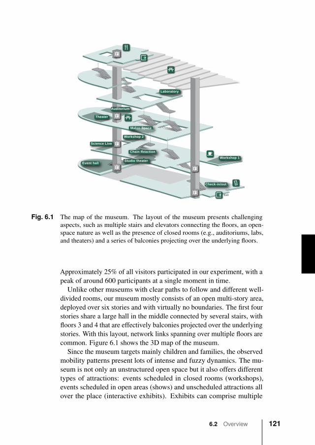
Event hall

Science Live

Workshop 2

Chain Reaction

Studio theater Workshop 1

Auditorium

Theater

Maker Space

Laboratory

Exit

Check-in/out

Fig. 6.1 The map of the museum. The layout of the museum presents challengingaspects, such as multiple stairs and elevators connecting the floors, an open-space nature as well as the presence of closed rooms (e.g., auditoriums, labs,and theaters) and a series of balconies projecting over the underlying floors.

Approximately 25% of all visitors participated in our experiment, with apeak of around 600 participants at a single moment in time.

Unlike other museums with clear paths to follow and different well-divided rooms, our museum mostly consists of an open multi-story area,deployed over six stories and with virtually no boundaries. The first fourstories share a large hall in the middle connected by several stairs, withfloors 3 and 4 that are effectively balconies projected over the underlyingstories. With this layout, network links spanning over multiple floors arecommon. Figure 6.1 shows the 3D map of the museum.

Since the museum targets mainly children and families, the observedmobility patterns present lots of intense and fuzzy dynamics. The mu-seum is not only an unstructured open space but it also offers differenttypes of attractions: events scheduled in closed rooms (workshops),events scheduled in open areas (shows) and unscheduled attractions allover the place (interactive exhibits). Exhibits can comprise multiple

6.2 Overview 121

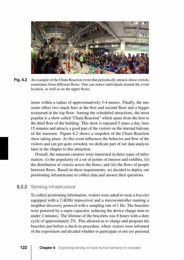
Fig. 6.2 An example of the Chain Reaction event that periodically attracts dense crowds,sometimes from different floors. One can notice individuals around the eventlocation, as well as on the upper floors.

items within a radius of approximatively 3-4 meters. Finally, the mu-seum offers two snack bars at the first and second floor and a biggerrestaurant at the top floor. Among the scheduled attractions, the mostpopular is a show called “Chain Reaction” which spans from the first tothe third floor of the building. This show is repeated 5 times a day, lasts15 minutes and attracts a good part of the visitors on the internal balconyof the museum. Figure 6.2 shows a snapshot of the Chain Reactionshow taking place. As this event influences the behavior and flow of thevisitors and can get quite crowded, we dedicate part of our data analysislater in the chapter to this attraction.

Overall, the museum curators were interested in three types of infor-mation: (i) the popularity of a set of points of interest and exhibits, (ii)the distribution of visitors across the floors, and (iii) the flows of peoplebetween floors. Based on these requirements, we decided to deploy ourpositioning infrastructure to collect data and answer their questions.

6.2.2 Sensing infrastructureTo collect positioning information, visitors were asked to wear a braceletequipped with a 2.4GHz transceiver and a microcontroller running aneighbor discovery protocol with a sampling rate of 1 Hz. The braceletswere powered by a super capacitor, reducing the device charge time tounder 2 minutes. The lifetime of the bracelets was 8 hours with a dutycycle of approximately 2%. This allowed us to charge and program thebracelets just before a check-in procedure, where visitors were informedof the experiment and decided whether to participate or not (no personal


environments

information was collected and all data was anonymized). The check-in/out procedure additionally created a unique entry in the databasewith a timestamp and the bracelet ID, that allowed us to remove anyexchanged messages between the anchor points and the bracelets thathad yet to be handed out.

Anchors. For each point of interest (PoI), an anchor device was in-stalled. These devices had the same hardware as the bracelets but weredifferent in two ways. First, they were running a modified version of ourneighbor discovery mechanism that did not require anchors to discovertheir neighborhood, but instead only to be discovered by the braceletsworn by the visitors. Second, anchors were powered by either a wallsocket or by a large battery back. Through a reliable source of power, itwas possible to run the neighbor discovery algorithm with longer dutycycles, increasing even more the probability of a PoI to be discoveredby bracelets. As a result we were able to discover bracelets in the rangeof a PoI in just a few seconds. Note that while for positioning purposesit is usually more reliable to instrument each PoI with an anchor, as wewill show for MONA this is not a necessary condition.

Every second, bracelets could receive broadcast from anchors orother bracelets within a distance of some 5-7 meters. Such broadcastscontain the unique identifier (ID) of the sender, and we consider thereception of such broadcast as a proximity detection between the twonodes involved. Bracelets recorded together with the ID of the othernode also signal strength information about the broadcast (which can beused as an approximation of the nodes’ distance).

Sniffers. Once every second, bracelets reported the proximity detec-tions collected during the previous second via a special packet sent ona dedicated channel to the backbone of the system consisting of thesniffers. Like anchors, sniffers used the same hardware as bracelets inaddition to a single-board computer that used either WiFi or Ethernet tocommit the packet to a central database hosted on a server. The snifferswere placed uniformly in the museum to cover all areas, with someoverlap.

Each sniffed packet could report up to three detections, favoringtwo anchors and one bracelet when possible. The resulting datasetwas collected over three days of experiments containing more than 17million anchor-to-bracelet and bracelet-to-bracelet detections, together

6.2 Overview 123

with timestamp and signal strength information. In this chapter, wefocus on the second day of experimentation.

6.2.3 Data analysisOnce data is collected by the sniffer and committed to the centraldatabase, it can be analyzed either in real-time or offline. Becauseof the mentioned irregularities of wireless communications, in particularat high density, the database presents a number of shortcomings, suchas missed detections and detections that are logically unexpected whenconsidering location and signal strength. We designed a filtering pipelineto overcome these artifacts and compute the positioning of the visitorsat PoIs at each time of their visit. The pipeline comprises two steps.

First, the set of proximity detections is filtered with a particle filter thattakes into account the topology of the museum, the positions of anchorsand PoIs, and the position and movements of the visitors wearing abracelet. This step drastically increases positioning accuracy comparedto more naive approaches, such as assigning visitors to the anchorsdetected with highest signal strength, but also allows positionings atPoIs that are not instrumented with an anchor (which is impossible withthe aforementioned naive approaches).

Second, we smoothen the positioning information with a density-based filter and a majority-voting filter, which remove some of theartifacts and oscillations left over by the particle filter. At the end of thepipeline, we are able to assign at each moment in time each visitor toa PoI, if any. We utilize this filtered dataset of positionings for furtheranalysis about PoIs popularity and flows between floors.

6.3 Related workThere is a large body of literature regarding indoor localization andpositioning with mobile sensors. In this section we first present existingwork regarding use of pervasive sensing technology in museums, andthen we describe existing efforts and limitations of indoor (cooperative)localizations systems.

Museum monitoring. In the case of monitoring and analyzing thebehavior of visitors in a museum, the visualization of metrics such aspopularity, attraction, holding power and flows has been explored tosupport the work of museum staff [85, 133]. Earlier works focus on


environments

localizing visitors at coarse-grained levels (room level) through tech-nologies like Bluetooth [162] to support multimedia guides [22, 149].Nevertheless, more complex sensors and localization techniques can beemployed to obtain a deeper understanding of crowd related phenomena.

A recent work, for example, utilizes “physiological” sensors and apositioning system based on RFID to classify the behavior of visitorsinto three categories: “the contemplative”, “the enthusiast”, and “thesocial experience” [78]. Similarly, the location and heading of pairs ofvisitors have been used to classify the visitor behavior early in their visitand to provide social-aware services to increase their engagement [42].Differently from these approaches, our work does not focus on a classi-fication task but it tries to quantify the behavior of visitors throughoutthe whole museum area. Moreover, our work extends existing workenabling measurements in scenarios where the sequence and boundariesof exhibits are not clearly defined.

An alternative approach to crowd monitoring with mobile and wear-able sensors is to use cameras. Computer-vision techniques are a com-mon approach to tracking human mobility [166, 130, 161] and detectinganomalies in a crowd [103, 81, 148]. However, cameras can suffer frompoor lighting, and temporary or permanent obstructions [166]. Also,fusing the views from multiple cameras together in a highly dynamicindoor scenario is quite challenging [128]. Finally, the privacy issue ofcollecting large-scale footage of visitors often restricts researchers fromaccessing these sources of data (as in our case).

Indoor localization. A simple way of monitoring a crowd consists inprecisely tracking the absolute position of each individual. While thistechnique is a feasible option in outdoor scenarios – where the GPSsystem can be exploited – for indoor conditions accurate localization isstill an open problem.

Among the wide literature of radio-based localization techniques,only few [118, 14, 90] are accurate enough to be employed in museumscenarios. Unfortunately, none of these techniques perform consistentlythroughout the museum areas. It is known, in fact, that the localizationerror increases significantly at the edges of rooms and in hallways [94],conditions that are often present in museum topologies. For our trackingapplication, this phenomenon can be even more problematic, since evensmall estimation errors could lead to visitors being associated to thewrong exhibit, positioned in the wrong room or placed on the wrongfloor.

6.3 Related work 125

An additional problem of indoor localization techniques is that thelocation of a device is often estimated by comparing the current radio ob-servations with a fingerprint obtained at deployment time. Unfortunately,in crowd monitoring applications, the ever-changing conditions of themuseum and the crowd can drastically affect the network connectivity,undermining the efficacy of fingerprint comparisons. Changes in thefurniture location, for example, could lead to different multi-path effectsand, thus, different radio fingerprints [94] and hence require recomput-ing fingerprints of the environment. Moreover, radio characteristics suchas the received signal strength can be significantly influenced by thedensity of the crowd, up to the point that this relation is exploited bysome mechanisms to estimate the crowd density [163, 105].

We borrow some ideas from the field of cooperative localization [150,157, 108]. In cooperative localization, nodes cooperate and share mea-surement information to increase their localization accuracy in a peer-to-peer manner. Typical information being shared between nodes is thegeographical topology and some measurements regarding the communi-cation between nodes with known and unknown locations. In contrast,we are not interested in deploying algorithms that can be computed ina distributed manner by the nodes “in-the-network”. We focus insteadon computing bracelet positions through a dedicated central repository,leveraging a more global and complete view without being limited bynetwork topology. This aspect is particularly useful in high densityscenarios, where packet loss increases, potentially hindering cooperativeapproaches.

Finally, many of these approaches are usually tested outside of theextreme conditions of high mobility and density of a complex real-worldmuseum as the one subject to our study.

6.4 Model

We consider N visitors V = {v1,v2, . . . ,vN}, each wearing a braceletduring the visit and being uniquely identifiable during the T seconds ofduration of the day (in our case, from 10AM to 6PM). While braceletshave their unique IDs and were re-used during the experiment, each ele-ment in V has a unique ID assigned at check-in, and we use these IDs fordetections. The museum has O points of interest I = {i1, i2, . . . , iO} andM anchors A = {a1,a2, . . . ,aM}. In the simple case where each anchoris assigned to a PoI, I ≡ A. We consider S the set of proximity sensorsS =V ∪A = {s1,s2, . . . ,sN+M}, as the union of detectable anchors and


environments

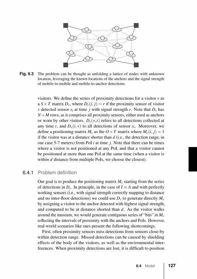
Fig. 6.3 The problem can be thought as unfolding a lattice of nodes with unknownlocation, leveraging the known locations of the anchors and the signal strengthof mobile-to-mobile and mobile-to-anchor detections.

visitors. We define the series of proximity detections for a visitor v asa S×T matrix Dv, where Dv(i, j) = r if the proximity sensor of visitorv detected sensor si at time j with signal strength r. Note that Dv hasN+M rows, as it comprises all proximity sensors, either used as anchorsor worn by other visitors. Dv(∗, t) refers to all detections collected atany time t, and Dv(i,∗) to all detections of sensor si. Moreover, wedefine a positioning matrix Mv as the O×T matrix where Mv(i, j) = 1if the visitor was at a distance shorter than d (i.e., the detection range, inour case 5-7 meters) from PoI i at time j. Note that there can be timeswhere a visitor is not positioned at any PoI, and that a visitor cannotbe positioned at more than one PoI at the same time (when a visitor iswithin d distance from multiple PoIs, we choose the closest).

6.4.1 Problem definitionOur goal is to produce the positioning matrix Mv starting from the seriesof detections in Dv. In principle, in the case of I ≡ A and with perfectlyworking sensors (i.e., with signal strength correctly mapping to distanceand no inter-floor detections) we could use Dv to generate directly Mv

by assigning a visitor to the anchor detected with highest signal strength,and computed to be at distance shorted than d. As the visitor walksaround the museum, we would generate contiguous series of “bits” in Mv

reflecting the intervals of proximity with the anchors and PoIs. However,real-world scenarios like ours present the following shortcomings.

First, often proximity sensors miss detections from sensors close-bywithin detection range. Missed detections can be caused by shieldingeffects of the body of the visitors, as well as the environmental inter-ferences. When proximity detections are lost, it is difficult to position

6.4 Model 127

the visitor at PoIs. Second, proximity sensors can collect ambiguousdetections, for example, from anchors spatially close-by but at the otherside of a wall or at a different floor. Note that these proximity detectionsare often received at a high signal strength, so they can generate wrongpositionings. Moreover, due to tunneling effects, spurious proximitydetections can also happen, though more rarely, between sensors furtherthan the expected transmission range (tens of meters). Third, signalstrength is unreliable and noisy as a proxy for distance estimation, asit can vary given the same distance between visitors and anchors de-pending, for example, on the crowd density as well as the museumtopology.

Finally, in real-world scenarios it is not always possible to instrumentevery PoI with a corresponding anchor node. Anchors are instead spreadover the museum (for positioning purposes) and installed in convenientlocations, without being associated to a particular PoI. In this case, it ispossible to position visitors at un-instrumented PoIs by exploiting thedetections of close-by sensors, which can be both fixed (other anchors)or mobile (other visitors), and whose sensing range overlaps over theun-instrumented PoI.

In principle, the problem can in fact be thought as the unfoldinga lattice of nodes with unknown locations, connected by edges withweight proportional to the strength of the respective mobile-to-mobiledetections, by leveraging the known location of the anchors and thestrength of mobile-to-anchor detections1.

Note that this aspect of MONA has commonalities with some indoorlocalization techniques, but has the simpler goal of assigning a visitor tothe closest PoI within distance d, and not necessarily a precise absoluteposition (although it may require to estimate one as a step to achievesuch goal). To a certain extent, our task can be thought as computinga more coarse-grained location within the specific boundaries of theanchors in the local areas of the museum.

6.4.2 Particle filterWe designed and implemented a particle filter that takes into accountthe topology of the museum, the location of anchors and PoIs, and theestimated location and movement of the visitors. Particle filters havebeen successfully used in indoor localization to estimate the absoluteposition of individuals with unreliable sensors [56, 63]. For localization,

1In this sense, the problem is also analogous to the embedding of a graph through astring-based force-model.


environments

usually a mobile sensor communicates with a few anchors installed atknown locations. It is assumed that the sensor can communicate with all,or a majority of, anchors from all positions and directions, and that thesensor can measure distance from these anchors, for example, throughsignal strength or time-of-flight. Our setup is more complex, as we havea larger number of anchors that are detectable at shorter distance, and anumber of detections from proximity sensors at unknown locations, i.e.,the visitors, together with a multi-story venue.

The filter requires topology information about the museum, such asthe sets of anchors A and PoIs I, each defined by a triple f ,x,y with fbeing the floor number and x,y the coordinate within that floor, and aset of walls W = {w1,w2, . . . ,wM}, each defined as a segment betweentwo points. Every floor is modeled as a distinct two-dimensional space,with an independent origin. As floors are connected by a number ofdifferent stairs and elevators, it is difficult to model the transition spacesbetween floors reliably. Instead, as we discuss later in this section, weassume a visitor can “appear” at a certain floor and model this transitionconfidence in the filter, based on the measurement. For each visitor wedefine a set of particles P = {p1, p2, . . . , pK}, each defined by a tuplef ,x,y and a weight w that models the likelihood of the visitor to be atthat coordinate. Initially, particles are spread uniformly at random acrossthe museum floors.

For each time of the day 0 ≤ t < T , the following four steps areexecuted for each visitor checked-in at that time, given the respectivedetection matrix Dv.

• Estimation: At each time, we estimate the floor the visitor ispositioned at, if any, by computing the floor with the largestnumber of particles (normalized by floor sizes), given enoughconfidence is provided by the particles. Then, we compute thelikelihood of each particle’s estimate (i.e., its position) given themeasurement at time t, that is the set of detections in Dv containedin the t-th column. For each particle p, the weight is updatedusing the likelihood function Φ(p,Dv(∗, t)). More details aboutthis step are given later in this section.

• Positioning: We estimate the position of v by computing theweighted average among the floor’s particles (i.e., the centroid)and find the closest PoI ii on the floor within distance d. We thenset Mv(i, t) = 1, unless the confidence of the estimate is smallerthan a threshold δ .

6.4 Model 129

• Re-sampling: We create a new set of particles by drawing withreplacement from the current weighted set of particles. Whiledrawing particles from the set, we favor particles proportionallyto their weight (i.e., their likelihood). As a result, particles withhigher likelihood are picked more often than particles with lowerlikelihood. Depending on the confidence in the current set ofparticles, we may choose to (i) pick only from the particles inthe current floor, (ii) additionally spread particles with smallerlikelihood across other floors, or (iii) re-distribute all particlesacross all floors (i.e., when we believe we have lost track of thevisitor). More details about this step is given later in this section.

• Movement: We move particles at walking speed in random direc-tions, avoiding illegal moves, such as walking through walls.

Compared, for example, to previous work on positioning [100] (seeChapter 5), the two steps where we focused most of our efforts to tailorthe filter for our use-case are the estimation and the re-sampling steps.Those steps were redesigned to (i) include mobile-to-mobile detections,(ii) consider multi-floor environments, (iii) support PoIs without anchorsand anchors not associated to PoI, and (iv) omni-directional sensingwith signal strength.

In general, we can compute the confidence of the particles’ centroidby measuring the dispersion of the particles and the amount of timespent without collecting any detection from a sensor located on the samefloor as the visitor. We consider the visitor to be at the floor with thelargest number of particles, normalized by floor sizes, given enoughconfidence. Note that having a visitor assigned to a floor does not meanwe position the visitor at any PoI, as that depends on the position of theparticles within the floor, their likelihood, and dispersion.

Likelihood function Φ(p,Dv(∗, t)) computes the likelihood of particlep given the set of sensors detected at time t that were positioned on thesame floor as p. In Φ we consider both anchors, of which we know thelocation, and neighbor visitors, for which we use the centroid computedat time t − 1. In other words, we use neighbor visitors as anchors.We consider neighbor visitors only if we are confident enough of theircentroid.

Intuitively, the likelihood of a particle depends on the particle’s dis-tance from a reference point proportionally to the strength of the detec-tions. This reference point can be a single sensor or an average acrosssensors. We compute the reference point and the distance from it asfollows. We first map signal strength values to the (0,1] continuous


environments

interval by means of a Gaussian kernel2. Then, if multiple sensors weredetected, we compute the average coordinate across these sensors’ coor-dinates weighted by the respective signal strength, and use the particle’sdistance from this average coordinate. We use a linear kernel to mapdistances to the (0,1] continuous interval.

If only one sensor was detected, instead, we compute the differencebetween the signal strength value and the particle distance from the sen-sor (both mapped to the (0,1] continuous interval through the respectivekernels), and use this difference. Note that while single-sensor reportsare more common, the system is still practically multi-laterating overtime, as particles that are more coherent with a series of measurementsreceive a higher likelihood.

When we update particle weights and re-sample the particles, weproceed depending on the centroid confidence c as follows (the twothresholds δ and δ ′ to be chosen empirically).

• c > δ : This means we know the visitor is on the floor. Weignore the likelihood of particles from other floors, practically“teleporting” these particles from other floors to the current one.

• δ ′ < c≤ δ : This means we are starting to believe the visitor mayhave left the floor. We spread particles with smaller likelihoodfrom the current floor to other floors.

• c ≤ δ ′: This means we have lost the visitor completely. Were-distribute particles uniformly at random across floors.

As a visitor moves around a floor, particles spread towards areas thatare more likely to have produced the current measurement. As the visitormoves to a new floor, absence of detections on the previous floor causesparticles to disperse until we start spreading particles on the other floors,including the new one.

6.4.3 Smoothening

The particle filter is able to drastically increase positioning accuracy.Yet, some artifacts, such as short jumps to a PoI nearby or on anotherfloor, are still possible though rare. These jumps produce gaps in thebursts of positionings as well as spurious positionings. We apply theremaining two smoothening steps of our positioning pipeline comprisinga density-based filter and a majority-voting filter.

First, we apply a density-based filter [98] (see Chapter 4) to all therows of Mv. The filter computes statistics about positioning information

2signal strength decreases non-linearly with distance

6.4 Model 131

at different PoIs over time, and clusters them together. These clustersof positionings are effectively intervals of time where the visitor was inproximity to a PoI. Once these intervals are identified, the filter fills thegaps in these intervals, and ignores the noisy positionings. One can thinkof this filter as a low-pass filter implemented with a sliding window, butthe optimal parameters of the low-pass filter are chosen automatically.

Then, we pass a majority-voting filter on the data produced by theprevious stage. The filter slides a window of L seconds of duration aheadof, and including, t over all rows to decide at which PoI to position v. Thefilter decides by choosing the PoI with the largest number of positioningsin that window of time, and breaks ties by choosing the PoI chosen atthe previous window (or randomly if none was chosen at that time).

6.5 Evaluation

6.5.1 MethodologyBefore the 3-days main experiment, we conducted a controlled exper-iment where we scripted a visit of the first floor while the completesensing infrastructure in the museum was turned on. The script definedarrival and departure times at each PoI. Originally, the first floor had allPoIs associated with an anchor, and one additional anchor to improve po-sitioning accuracy. To test the ability to position visitors at PoIs withoutanchors, we added to the script three “virtual” PoIs not associated withany particular exhibit or anchor (that is, solely defined by a coordinatein space). In addition, one PoI with an anchor was not used in the script,but the anchor was turned on and hence could affect accuracy.

Together with the scripted visit, we distributed 15 bracelets aroundeach interested PoI area within a radius of some 15-20 meters from therespective anchor (or virtual PoI coordinate), at 1 meter of height, andmoved them at random across the space for the whole duration of thestop. This setup allowed us to control bracelet density and movement,and at the same time minimize external factors like body shieldingeffects (which were tested during the real-world experiment). Each stoplasted eight minutes, divided in four slots of two minutes. During thefirst slot only the visitor’s bracelet was on, while during the following 3slots we turned on the additional bracelets, in groups of 5 per slot.

To evaluate real-world accuracy, for the duration of the main ex-periment we positioned 5 bracelets at known locations at PoIs, andadditionally scripted a visit of the whole museum of the duration ofaround one and a half hours with 14 stops of the duration of around


environments

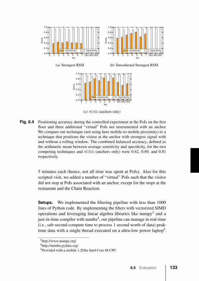
0 1 2 3 4 5 6 7 VR1 VR2 VR3PoI

0.0

0.2

0.4

0.6

0.8

1.0

Sco

re

Sensitivity Specificity

(a) Strongest RSSI

0 1 2 3 4 5 6 7 VR1 VR2 VR3PoI

0.0

0.2

0.4

0.6

0.8

1.0

Sco

re


(b) Smoothened Strongest RSSI

0 1 2 3 4 5 6 7 VR1 VR2 VR3PoI

0.0

0.2

0.4

0.6

0.8

1.0Sco

re


(c) MONA (anchors only)

Fig. 6.4 Positioning accuracy during the controlled experiment at the PoIs on the firstfloor and three additional “virtual” PoIs not instrumented with an anchor.We compare our technique (not using here mobile-to-mobile proximity) to atechnique that positions the visitor at the anchor with strongest signal withand without a rolling window. The combined balanced accuracy, defined asthe arithmetic mean between average sensitivity and specificity, for the twocompeting techniques and MONA (anchors only) were 0.62, 0.69, and 0.81respectively.

5 minutes each (hence, not all time was spent at PoIs). Also for thisscripted visit, we added a number of “virtual” PoIs such that the visitordid not stop at PoIs associated with an anchor, except for the stops at therestaurant and the Chain Reaction.

Setups. We implemented the filtering pipeline with less than 1000lines of Python code. By implementing the filters with vectorized SIMDoperations and leveraging linear algebra libraries like numpy3 and ajust-in-time compiler with numba4, our pipeline can manage in real-time(i.e., sub-second compute time to process 1 second worth of data) peak-time data with a single thread executed on a ultra-low power laptop5.

3http://www.numpy.org/4http://numba.pydata.org/5Provided with a mobile 1.2Ghz Intel Core M CPU

6.5 Evaluation 133

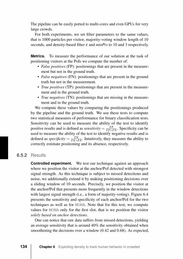
The pipeline can be easily ported to multi-cores and even GPUs for verylarge crowds.

For both experiments, we set filter parameters to the same values,that is 1000 particles per visitor, majority-voting window length of 10seconds, and density-based filter ε and minPts to 10 and 3 respectively.

Metrics. To measure the performance of our solution at the task ofpositioning visitors at the PoIs we compute the number of:

• False positives (FP): positionings that are present in the measure-ment but not in the ground truth.

• False negatives (FN): positionings that are present in the groundtruth but not in the measurement.

• True positives (TP): positionings that are present in the measure-ment and in the ground truth.

• True negatives (TN): positionings that are missing in the measure-ment and in the ground truth.

We compute these values by comparing the positionings producedby the pipeline and the ground truth. We use these tests to computetwo statistical measures of performance for binary classification tests.Sensitivity can be used to measure the ability of the test to identifypositive results and is defined as sensitivity = T P

T P+FN . Specificity can beused to measure the ability of the test to identify negative results and isdefined as specificity = T N

T N+FP . Intuitively, they measure the ability tocorrectly estimate positioning and its absence, respectively.

6.5.2 ResultsControlled experiment. We test our technique against an approachwhere we position the visitor at the anchor/PoI detected with strongestsignal strength. As this technique is subject to missed detections andnoise, we additionally extend it by making positioning decisions overa sliding window of 10 seconds. Precisely, we position the visitor atthe anchor/PoI that presents more frequently in the window detectionswith largest signal strength (i.e., a form of majority-voting). Figure 6.4presents the sensitivity and specificity of each anchor/PoI for the twotechniques as well as for MONA. Note that for this test, we computevalues for MONA only for the first slot, that is we position the visitorsolely based on anchor detections.

One can notice that raw data suffers from missed detections, yieldingan average sensitivity that is around 40% the sensitivity obtained whensmoothening the decisions over a window (0.42 and 0.68). As expected,


environments

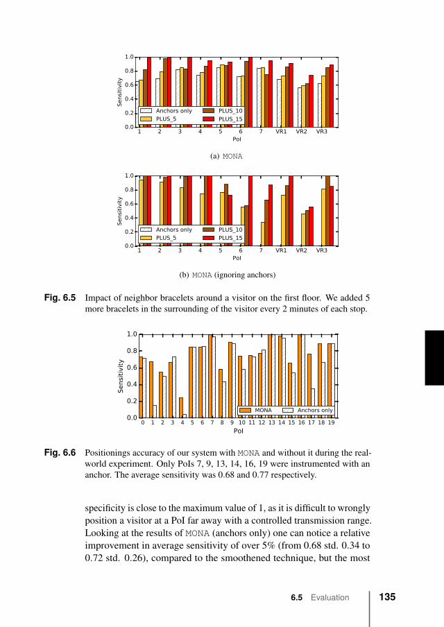
1 2 3 4 5 6 7 VR1 VR2 VR3PoI

0.0

0.2

0.4

0.6

0.8

1.0

Sensitivity

Anchors only

PLUS_5

PLUS_10

PLUS_15

(a) MONA

1 2 3 4 5 6 7 VR1 VR2 VR3PoI

0.0

0.2

0.4

0.6

0.8

1.0

Sensitivity

Anchors only

PLUS_5

PLUS_10

PLUS_15

(b) MONA (ignoring anchors)

Fig. 6.5 Impact of neighbor bracelets around a visitor on the first floor. We added 5more bracelets in the surrounding of the visitor every 2 minutes of each stop.

0 1 2 3 4 5 6 7 8 9 10 11 12 13 14 15 16 17 18 19

PoI

0.0

0.2

0.4

0.6

0.8

1.0

Sensitivity

MONA Anchors only

Fig. 6.6 Positionings accuracy of our system with MONA and without it during the real-world experiment. Only PoIs 7, 9, 13, 14, 16, 19 were instrumented with ananchor. The average sensitivity was 0.68 and 0.77 respectively.

specificity is close to the maximum value of 1, as it is difficult to wronglyposition a visitor at a PoI far away with a controlled transmission range.Looking at the results of MONA (anchors only) one can notice a relativeimprovement in average sensitivity of over 5% (from 0.68 std. 0.34 to0.72 std. 0.26), compared to the smoothened technique, but the most

6.5 Evaluation 135

interesting result is the impact on positioning at virtual PoIs (impossiblewith the other techniques). This is due to the spatial nature of the filter.

Figure 6.5(a) presents the sensitivity results when MONA takes intoaccount also detections of neighbor bracelets to position both the visitorand the neighbor bracelets. We do not present specificity values hereas they are consistently close to 1 as in Figure 6.4. One can notice thatadding mobile node proximity information improves positioning abilityreaching a value of (or close to) 1 when 15 additional neighbors are used,with an average relative improvement between using only anchors andincluding 15 neighbors of around 30% (from average sensitivity of 0.72std. 0.09 to average sensitivity of 0.94 std. 0.08). The improvement isslightly worse in the case of virtual PoIs (in particular VR2), but notethat here we leveraged the anchors used for the other PoIs (except foronly an additional anchor). Moreover, more data points (i.e., visits)should yield more statistically consistent results (e.g., for PoI 7 and3 adding 10 bracelets yields worse results than using anchors only).Finally, one would expect a slightly lower impact in the real world,where body shielding effects and other irregularities would influencemobile-to-mobile detections.

To show the impact of mobile-to-mobile proximities, we compute thesame results but ignoring anchor detections completely for the scriptedvisit. That is, we position the visitor only based on mobile-to-mobiledetections, but position the neighbor bracelets based on both mobile-to-mobile and mobile-to-anchor detections. Clearly, this setup could not bedeployed and is used only for testing purposes. Figure 6.5(b) presentsthe results of this test.

First, all values for the first slots are 0, as no anchor detections areavailable. Second, for certain PoIs the results are better than for Fig-ure 6.5(a). This result may seam counterintuitive at first, as we are usingless information (i.e., the anchors detections). However, the reason isto be found in the “averaging” effect performed by the neighbors. Infact, the positioning of the visitor cannot be affected by noisy detectionsfrom anchors far away but it is based only on the neighbors that areconsistently positioned by the filter around the area (and those few thattemporarily are not, are “filtered out” by those that are). Third, for somePoIs the performance is much worse, again in particular VR2. In general,these results shows how local mobile-to-mobile proximity detectionscan overcome missed detections from anchors, which tend to increasewhen crowd density increases.


environments

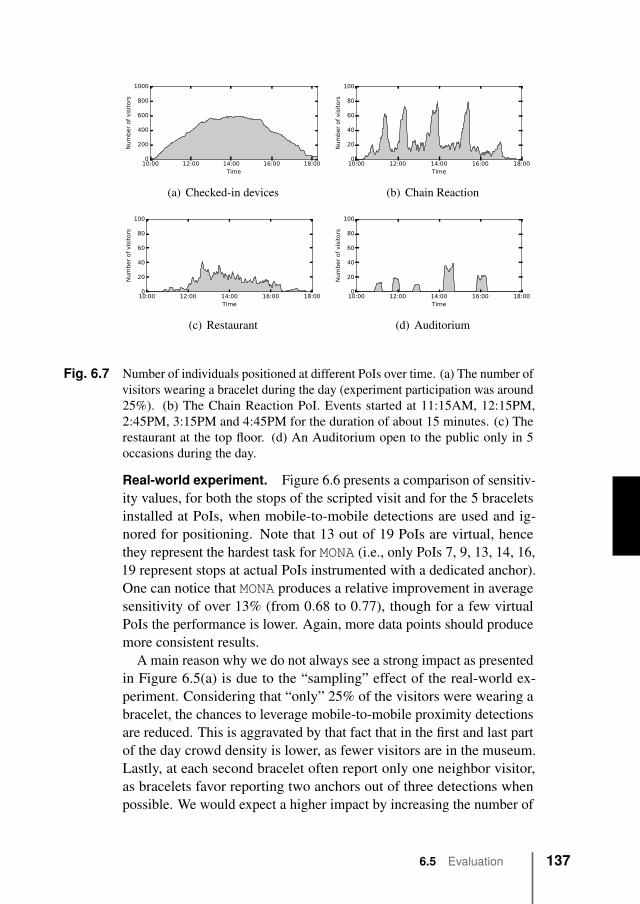
10:00 12:00 14:00 16:00 18:00Time

0

200

400

600

800

1000

Num

ber

of

vis

itors

(a) Checked-in devices

10:00 12:00 14:00 16:00 18:00Time

0

20

40

60

80

100

Num

ber

of

vis

itors

(b) Chain Reaction

10:00 12:00 14:00 16:00 18:00Time

0

20

40

60

80

100

Num

ber

of

vis

itors

(c) Restaurant

10:00 12:00 14:00 16:00 18:00Time

0

20

40

60

80

100

Num

ber

of

vis

itors

(d) Auditorium

Fig. 6.7 Number of individuals positioned at different PoIs over time. (a) The number ofvisitors wearing a bracelet during the day (experiment participation was around25%). (b) The Chain Reaction PoI. Events started at 11:15AM, 12:15PM,2:45PM, 3:15PM and 4:45PM for the duration of about 15 minutes. (c) Therestaurant at the top floor. (d) An Auditorium open to the public only in 5occasions during the day.

Real-world experiment. Figure 6.6 presents a comparison of sensitiv-ity values, for both the stops of the scripted visit and for the 5 braceletsinstalled at PoIs, when mobile-to-mobile detections are used and ig-nored for positioning. Note that 13 out of 19 PoIs are virtual, hencethey represent the hardest task for MONA (i.e., only PoIs 7, 9, 13, 14, 16,19 represent stops at actual PoIs instrumented with a dedicated anchor).One can notice that MONA produces a relative improvement in averagesensitivity of over 13% (from 0.68 to 0.77), though for a few virtualPoIs the performance is lower. Again, more data points should producemore consistent results.

A main reason why we do not always see a strong impact as presentedin Figure 6.5(a) is due to the “sampling” effect of the real-world ex-periment. Considering that “only” 25% of the visitors were wearing abracelet, the chances to leverage mobile-to-mobile proximity detectionsare reduced. This is aggravated by that fact that in the first and last partof the day crowd density is lower, as fewer visitors are in the museum.Lastly, at each second bracelet often report only one neighbor visitor,as bracelets favor reporting two anchors out of three detections whenpossible. We would expect a higher impact by increasing the number of

6.5 Evaluation 137

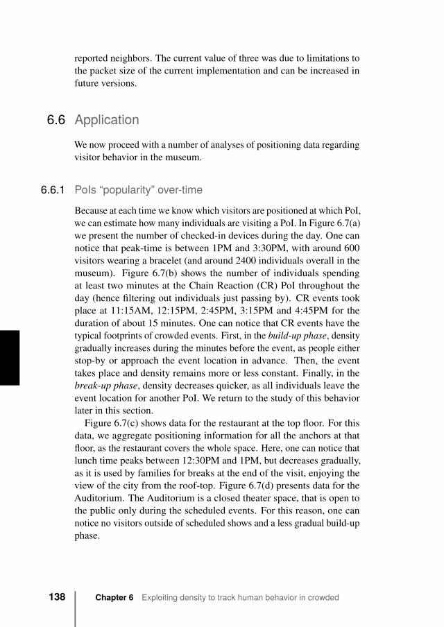
reported neighbors. The current value of three was due to limitations tothe packet size of the current implementation and can be increased infuture versions.

6.6 Application

We now proceed with a number of analyses of positioning data regardingvisitor behavior in the museum.

6.6.1 PoIs “popularity” over-time

Because at each time we know which visitors are positioned at which PoI,we can estimate how many individuals are visiting a PoI. In Figure 6.7(a)we present the number of checked-in devices during the day. One cannotice that peak-time is between 1PM and 3:30PM, with around 600visitors wearing a bracelet (and around 2400 individuals overall in themuseum). Figure 6.7(b) shows the number of individuals spendingat least two minutes at the Chain Reaction (CR) PoI throughout theday (hence filtering out individuals just passing by). CR events tookplace at 11:15AM, 12:15PM, 2:45PM, 3:15PM and 4:45PM for theduration of about 15 minutes. One can notice that CR events have thetypical footprints of crowded events. First, in the build-up phase, densitygradually increases during the minutes before the event, as people eitherstop-by or approach the event location in advance. Then, the eventtakes place and density remains more or less constant. Finally, in thebreak-up phase, density decreases quicker, as all individuals leave theevent location for another PoI. We return to the study of this behaviorlater in this section.

Figure 6.7(c) shows data for the restaurant at the top floor. For thisdata, we aggregate positioning information for all the anchors at thatfloor, as the restaurant covers the whole space. Here, one can notice thatlunch time peaks between 12:30PM and 1PM, but decreases gradually,as it is used by families for breaks at the end of the visit, enjoying theview of the city from the roof-top. Figure 6.7(d) presents data for theAuditorium. The Auditorium is a closed theater space, that is open tothe public only during the scheduled events. For this reason, one cannotice no visitors outside of scheduled shows and a less gradual build-upphase.


environments

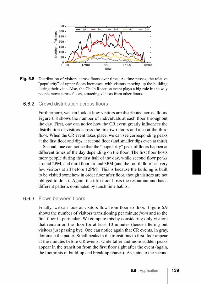
10:00 12:00 14:00 16:00 18:00Time

0

50

100

150

200

250

300

350

Number of visitors

1st 2nd 3rd 4th 5th

Fig. 6.8 Distribution of visitors across floors over time. As time passes, the relative“popularity” of upper floors increases, with visitors moving up the buildingduring their visit. Also, the Chain Reaction event plays a big role in the waypeople move across floors, attracting visitors from other floors.

6.6.2 Crowd distribution across floorsFurthermore, we can look at how visitors are distributed across floors.Figure 6.8 shows the number of individuals at each floor throughoutthe day. First, one can notice how the CR event greatly influences thedistribution of visitors across the first two floors and also at the thirdfloor. When the CR event takes place, we can see corresponding peaksat the first floor and dips at second floor (and smaller dips even at third).

Second, one can notice that the “popularity” peak of floors happen atdifferent times of the day depending on the floor. The first floor hostsmore people during the first half of the day, while second floor peaksaround 2PM, and third floor around 3PM (and the fourth floor has veryfew visitors at all before 12PM). This is because the building is builtto be visited somehow in order floor after floor, though visitors are notobliged to do so. Again, the fifth floor hosts the restaurant and has adifferent pattern, dominated by lunch time habits.

6.6.3 Flows between floorsFinally, we can look at visitors flow from floor to floor. Figure 6.9shows the number of visitors transitioning per minute from and to thefirst floor in particular. We compute this by considering only visitorsthat remain on the floor for at least 10 minutes (hence filtering outvisitors just passing by). One can notice again that CR events, in gray,dominate the patter. Small peaks in the transitions to first floor appearat the minutes before CR events, while taller and more sudden peaksappear in the transition from the first floor right after the event (again,the footprints of build-up and break-up phases). As stairs to the second

6.6 Application 139

10:00 12:00 14:00 16:00 18:00Time

0

2

4

6

8

10

12

Num

ber

of

vis

itors

reaching 1st leaving 1st

Fig. 6.9 Flow of visitors from and to the first floor. One can notice the influence of theChain Reaction, as visitors tend to leave the floor by the stairs close-by theattraction after the event, and approach the floor from the other floors beforethe event.

floor are positioned right besides the CR event location, visitors tend tomove to the second floor right after the event finishes.

6.7 DiscussionRegarding positioning accuracy, MONA uses mobile-to-mobile detec-tions not only to fight density, but to leverage it and yield better results.Moreover, MONA can position visitors also at PoIs not instrumented withanchors. To improve this second task, one can increase the number ofanchors around the museum, but it is an open question how to choosesuch locations in the most effective way. Increasing anchor density lo-cally to specific areas, perhaps those hosting more exhibits and attractinghigher visitor densities, should be a valid heuristic, but more research isnecessary to understand what factors can influence such decision.

Being in close proximity to an attraction does not necessarily meanthe visitor is paying attention to that particular attraction. Comparedto spaces hosting paintings and other visual arts, the attractions of themuseum were interactive and invited visitors to move around. Visitorswere not required to face a particular direction, as in the case of a canvason a wall. It can hence sometimes be erroneous to infer popularity justby counting the number of individuals at a certain PoI. For example,we noticed that PoIs close-by the CR event location present a smallincrease in the number of positionings when most crowded CR eventsare taking place. This could be caused by individuals that needed tostand further from the CR event location due to a large audience, insidethe proximity range of those PoIs, It is difficult to design a sensor thatis able to measure proximity in the complete surrounding of a visitor,


environments

as it is necessary in museums like the one where we ran our study, andat the same time face-to-face proximity, as required by other types ofattractions and analyses.

The data we presented shows clear behavioral trends, yet it is notalways obvious how museum staff can turn such insights into action.The museum staff re-organizes and re-furbishes the space every day,changing event schedules and locations as needed and depending onexpected types and numbers of individuals. There are hence plentyof opportunities for the staff to make more data-driven decisions. Forexample, too large audiences at the CR event could be avoided byorganizing other events in different locations at the same time, a strategyused by crowd management teams at music festivals.

A topic related to intervention is prediction. A number of differentmodels exist to synthesize and predict the behavior of a crowd on thetopic of evacuation, pedestrian mobility, and crowd dynamics [148].While some of these topics are of interest to museum staff, such as thoserelated to the safety of the visitors, none of them includes the particularnuances that characterize the entertaining and educational experienceof a museum. Ad hoc models need to be developed and fed with sensordata, to better understand and predict how visitors react to the decisionsof the museum staff. To this end, it may be necessary to fuse proximitydata with data coming from other sensors, like accelerometers [99] (seeChapter 7) and physiological sensors [78], that can offer insights aboutdifferent dimensions of the internal response of the visitors.

Finally, the experience of a museum does not start and end necessaryinside the building. Long queues and congestions outside the museumare of great importance to the overall experience of a visit as well as tosafety. Algorithms to predict and detect specific crowd dynamics suchas pedestrian flows, queues, or clogging outside or at the periphery ofthe museum are still missing, and would be relevant to the more generalfield of crowd management as well [97] (see Chapter 3).

6.8 Conclusions

We have presented the design and evaluation of a positioning systemthat leverages mobile-to-mobile proximity sensing to overcome missedmobile-to-anchor detections due to high crowd density. We have shownthat our approach is able to increase positioning accuracy when morevisitors wearing a proximity sensors are present in the museum. Themuseum where we conducted the study presented extreme conditions of

6.8 Conclusions 141

density and challenging conditions due to a complex multi-story openspace. We have tackled these challenges by tailoring a filtering pipelineto our use-case. Yet, the approach is general and applicable to anyproximity sensing technology that is able to detect neighbor sensorswith and an estimate of distance.

Moreover, we have used the data to gain insights about the behavior ofthe visitors during the experimentation days. The insights show a clearbehavioral trend, opening new questions regarding how museum staffcan integrate such an approach in their work. The work we presentedis however not limited solely to the use-case of a museum, but it isapplicable to the general problem of indoors crowd monitoring.


environments

7How was it? Exploiting smartphone sensing to measureimplicit audience responses tolive performances

„It’s not dangerous that computers startto think like men, but that men start tothink like computers.

— Sydney J. Harris

7.1 IntroductionThere is more to the behavior of a crowd than what can be observed fromthe external. Monitoring and understanding the internal response of acrowd to its environment, which includes other members of the crowd,any event happening in the surroundings, the location etc., can helppractitioners implement practices that increase the comfort and safetyof the crowd. For example, it can help the managers of a train stationschedule trains at platforms in a way that not only minimizes congestionsand density, but also distress. Moreover, it can help the organizers offestivals and parades, events where high density is a standard conditionalso in the most favorable cases (e.g., near a stage or in connectingroads), monitor whether such conditions are source of frustration, orworse of more extreme moods and emotions like panic.

An instrument providing information about the experience of an eventby a crowd opens a number of different applications that go beyondcrowd management. For example, the information about the experienceof an audience of a performance, and how it changes over time, could

The contents of this chapter have been originally published in “How was it? Ex-ploiting smart phone sensing to measure implicit audience responses to liveperformances” C. Martella, E. Gedik, L. Cabrera-Quiros, G. Englebienne, H. Hung- ACM Multimedia 2015, and have been slightly modified to improve readability.

143

help the designers of such performance gain feedback to improve theirproduction. Moreover, individual responses to performances could helporganizers, like theaters and museums, target individual customers withmarketing campaigns more effectively (e.g., recommend similar actswhen a positive response is detected).

Detecting the internal experience and response of a crowd throughspatio-temporal information is difficult, and perhaps proximity sensorsalone are not well suited to the task. Accelerometers, galvanic skinresponse sensors, and microphones are examples of pervasive sensorsthat have been explored in the past, and we focus on the former asthey are currently installed in most smart phones and hence suitable tolarge-scale pervasive measurements.

As we show in this chapter, it may not be sufficient to focus on theaccelerometric data of a single individual to understand her response, butit is necessary to look at the data of the group of individuals she belongsto as well. We need to understand how the whole crowd responses tomake sense of the individual experience of its members. This may benecessary to filter out irrelevant and noisy movements, and identify in-stead the salient moments where the movements have stronger meaning(i.e., in terms of internal response). Proximity information can playa role in this particular aspect, as we need to characterize the groupof people, and the part of the crowd, the individual is embedded in toperform such analysis.

We also show that response can be quantified by looking at the mo-ments before and after an event, which are often characterized by min-gling and networking activities (at least in social contexts). We show thatafter an even individuals can move differently during conversation, againrequiring to detect conversations and f-formations with spatio-temporalinformation in the first place.

Let us consider the example of the Chain Reaction event presented inthe previous chapter. We have shown that spatio-temporal informationenables the identification of when crowded events take place and theirduration, as well as the number of individuals involved. Furthermore, wehave shown that it is possible to recognize the typical fingerprints of thebuild-up and break-up phases, and how these influence density and flowsacross different floors. Yet, we are unaware of how individuals haveexperienced the events. We cannot analyze the data of all the visitorsall together, but we need to detect first the groups in the crowd that areattending different events, or are visiting different parts of location, to

144 Chapter 7 How was it? Exploiting smart phone sensing to measure

implicit audience responses to live performances

then perform higher-level behavioral and response analyses on thesesubgroups.

Contributions. More concretely, in this chapter make the followingcontributions. We show that (i) even when people are sitting and watch-ing a live dance performance, they spontaneously react it via bodymovements that can be captured from a standard acceleration sensor, (ii)moments of common spontaneous bodily reaction correspond to memo-rable events in the performance as reported by survey responses relatingto the performance, (iii) their reactions can be used to predict their enjoy-ment of the performance, whether they felt immersed in the experience,would recommend it to others, or thought dance performance changedtheir mood positively, (iv) and finally by considering the social contextthat surrounds the activity of going to a live dance performance, wealso provide initial results using acceleration and proximity sensors, thatsuggest that a change in the mood of a person as a result of watching alive dance performance is reflected in their general body behavior whilemingling.

7.2 Related workTraditional methods to investigate the response of an audience to a livedance performance make use of self-reports, such as surveys and in-terviews [21, 113]. Digital technologies can overcome the limitationsof surveys and interviews, by giving more direct and fine-grained in-sights into the response of an audience. For example, the explosionin popularity of the social media, e.g., Twitter, and mobile computinghas broadened the borders of a live performance, as fans comment andpost information and opinions live to the online community [16]. Practi-tioners are interested in the activity of their audience through the socialmedia to understand both their response and to leverage their activitiesas marketers of their performances [69, 88]. For example, some theaters,including Broadway, have experimented with so-called “tweet-seats”reserved for customers who promised to tweet about the performancelive [137].

Other rather less pervasive technologies can also overcome the granu-larity issues of surveys using sensors. For example, work in neuroaes-thetics use fMRI scanning to relate viewer responses to the aesthetics ofthe performance [20, 38, 24]. Moreover, tracking of eye gaze from videohas been used when trying to distinguish novice from expert observers

7.2 Related work 145

of dance [131]. Finally, physiological sensing such as galvanic skinresponse (GSR) sensors, have been investigated to measure the arousalof individuals watching a video of a dance performance, and its relation-ship with the individuals’ self-reports [86]. Similarly, GSRs have beenused also to measure the response to other types of live performance,such as comedy [144] and movies in a cinema [58].

These attempts show an increasing interest in quantifying the ex-perience of arts and cultural events, such as live dance performances.Unlike these approaches, we advocate the use of pervasive sensorswhich are readily available in smart phones, which enable less obtrusivemeasurements and on a massive scale, compared to those obtained viaphysiological sensing. In particular, in this work, we focus on usingacceleration and proximity sensors to measure people’s reactions to liveperformance, which have been used thus far to measure very differentphenomena.

Specifically, most work that consider accelerometers and people haveaddressed the problem of activity recognition of daily activities suchas walking, running, sitting, climbing the stairs [83], daily householdactivities including eating or drinking, vacuuming or scrubbing, lyingdown [12], or identifying modes of transportation taken [115]. There isa trend moving towards the detection of medically relevant events, suchas fall detection [46, 168], but all of these approaches focus resolutelyon physical activities where the behavior can be represented directly byquite specific movements of the body. It is possible to classify thesetypes of activities with excellent performance, yet these activities arevery different to analyzing the response to a live performance. Fewworks do exist where less specific body movements have been classified.For example, Matic et al. also used acceleration to detect speaking statusby strapping an accelerometer to the chest so that vibrations directlycaused by speaking could be detected [102], Hung et al. [71] usedbody movements to predict socially relevant actions with a device hungloosely round the neck or for detecting conversations[72]. Such workshighlight the potential of measuring spontaneous bodily responses toexternal stimuli using more pervasive sensing.

Apart from focusing on different activities and tasks, the above men-tioned works measure behavior in environments that are far less chal-lenging than a theater where the audience sits in silence, and where thelink between activity and behavior is not as direct. The most similarwork to our own was presented by Englebienne and Hung [53] whofound that they were able to identify audience members as professors



and non-professors from their behavior while attending an inaugurallecture. Although they were sitting, the small movements made in reac-tion to parts of the lecture demonstrated implicit responses of interest toparticular moments and content delivered during the lecture. However,they did not analyse whether reactions from the audience to the lecturecorrelated with enjoyment of the lecture, for example. Another closelyrelated work where the audience response was measured was presentedby Bao et al. [13] who investigated how users watching movies on abuffer tablet could have their implicit responses sensed by a wide varietyof modalities from the tablet itself including the video, audio, tabletinteractions, and accelerometer. In this case, movements from the tabletwhilst the user was holding it were used to gauge responses. Using amultimodal approach they were able to predict the rating of users tomovies they watched on the tablet. However, in this case, the user satalone to watch the movies and was not inhibited by the social normsusually adhered to in an auditorium.

7.3 Case study 1: direct responses to a performanceTo inspect whether it is possible to predict responses to a performance byusing data collected with wearable sensors, we have conducted an experi-ment in an actual dance performance. We start this section by explainingthe characteristics of the performance and the resulting dataset we ob-tained. Then, we describe the features we used in the data analysis andclassification experiments. The next two sections present the qualitativeanalysis and classification experiments we did based on questionnaireresponses. The qualitative analysis aims to show that the movementsof the audience are informative of their reactions to the performance.We do this by showing that the captured activity of the participantsand common responses correspond to the salient events happening inthe performance. The classification experiments present our methodol-ogy for automatically predicting a participant’s evaluation of the event.The performance and further analysis presented show that the proposedmethod is indeed promising and worth investigating further.

7.3.1 Data collectionThe sensor set-up. We organized a data collection experiment duringa dance performance. This event consisted of almost an hour and a halfof performance without intermission. It mainly consisted of dancingbut also included monologues by the performers in Italian, while the

7.3 Case study 1: direct responses to a performance 147

music was mainly based on live cello arrangements but also includedpre-recorded songs.

Using triaxial acceleration and IR cameras (for additional data veri-fication), we recorded 41 participants watching the performance. Theaccelerometers were located in a custom-made device hung aroundevery participant’s neck. These devices recorded at 20Hz and weresynchronized to a global time obtained by communicating through awireless network. However, due to hardware malfunctions, only 32accelerometers recorded data.

Furthermore, each device was equipped with a wireless radio, whichwe used to broadcast the device’s unique identifier (ID) every second upto a distance of some 2-3 meters. The reception of such broadcast bythe devices nearby can be considered a proximity detection. Since thedevice lies on the front of the chest, the radio transmission is shieldedby the body, hence restricting the proximity sensing mostly towards thefront of the individual. The device logs each detection on the on-boardstorage along with their timestamps. We used an energy-efficient MACprotocol [142] to allow the devices to communicate their IDs and detecteach other’s proximity.

In addition, the performance was recorded using a GoPro Hero +3 toanalyze salient moments (i.e., favorite moments that were reported bythe participants).

Survey responses. To evaluate the experience, a questionnaire wasfilled in by all 41 participants after the performance. Each questionnairehad 12 questions, where each group of three questions aimed to measureone aspect of the experience. The four aspects were “enjoyment”, “rec-ommendation (to a friend)”, “immersion” and “mood changes”. Eachparticipant evaluated these aspects of the performance on a ten-pointLikert scale, where one means "I completely disagree" and ten means "Icompletely agree". For measuring enjoyment, we adapted and selectedquestions presented in [124]. For the task of immersion, we selectedinvolvement questions from the group Presence Questionnaire [123].For recommendation we used items from O’Brien’s questionnaire [106].Each of these questions were carefully chosen to measure each taskand slightly adapted to match our scenario. We formed the questionsregarding mood by ourselves. Given that the majority of the audiencemembers were Dutch, we used a back-translation procedure to ensurethat each questionnaire item was accurately describing the original En-glish wording. This involved finding three different Dutch speakers



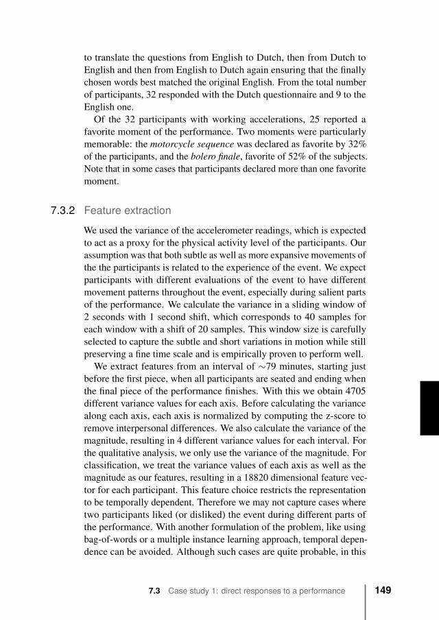
to translate the questions from English to Dutch, then from Dutch toEnglish and then from English to Dutch again ensuring that the finallychosen words best matched the original English. From the total numberof participants, 32 responded with the Dutch questionnaire and 9 to theEnglish one.

Of the 32 participants with working accelerations, 25 reported afavorite moment of the performance. Two moments were particularlymemorable: the motorcycle sequence was declared as favorite by 32%of the participants, and the bolero finale, favorite of 52% of the subjects.Note that in some cases that participants declared more than one favoritemoment.

7.3.2 Feature extractionWe used the variance of the accelerometer readings, which is expectedto act as a proxy for the physical activity level of the participants. Ourassumption was that both subtle as well as more expansive movements ofthe the participants is related to the experience of the event. We expectparticipants with different evaluations of the event to have differentmovement patterns throughout the event, especially during salient partsof the performance. We calculate the variance in a sliding window of2 seconds with 1 second shift, which corresponds to 40 samples foreach window with a shift of 20 samples. This window size is carefullyselected to capture the subtle and short variations in motion while stillpreserving a fine time scale and is empirically proven to perform well.

We extract features from an interval of ∼79 minutes, starting justbefore the first piece, when all participants are seated and ending whenthe final piece of the performance finishes. With this we obtain 4705different variance values for each axis. Before calculating the variancealong each axis, each axis is normalized by computing the z-score toremove interpersonal differences. We also calculate the variance of themagnitude, resulting in 4 different variance values for each interval. Forthe qualitative analysis, we only use the variance of the magnitude. Forclassification, we treat the variance values of each axis as well as themagnitude as our features, resulting in a 18820 dimensional feature vec-tor for each participant. This feature choice restricts the representationto be temporally dependent. Therefore we may not capture cases wheretwo participants liked (or disliked) the event during different parts ofthe performance. With another formulation of the problem, like usingbag-of-words or a multiple instance learning approach, temporal depen-dence can be avoided. Although such cases are quite probable, in this


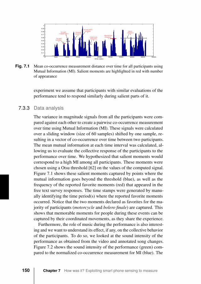
0 500 1000 1500 2000 2500 3000 3500 4000 4500 50000

0.1

0.2

0.3

0.4

0.5

0.6

0.7

0.8

0.9

1

time (sec)

bolerosequence

resurrection sequence motorcycle

sequence fun part(old lady)

maracassequence

fun part('naked man')

old lady kicks someone

3

1 1

3

8

8

5

Fig. 7.1 Mean co-occurrence measurement distance over time for all participants usingMutual Information (MI). Salient moments are highlighted in red with numberof appearance

experiment we assume that participants with similar evaluations of theperformance tend to respond similarly during salient parts of it.

7.3.3 Data analysisThe variance in magnitude signals from all the participants were com-pared against each other to create a pairwise co-occurrence measurementover time using Mutual Information (MI). These signals were calculatedover a sliding window (size of 60 samples) shifted by one sample, re-sulting in a vector of co-occurrence over time between two participants.The mean mutual information at each time interval was calculated, al-lowing us to evaluate the collective response of the participants to theperformance over time. We hypothesized that salient moments wouldcorrespond to a high MI among all participants. These moments werechosen using a Otsu threshold [62] on the values of the computed signal.Figure 7.1 shows these salient moments captured by points where themutual information goes beyond the threshold (blue), as well as thefrequency of the reported favorite moments (red) that appeared in thefree text survey responses. The time stamps were generated by manu-ally identifying the time period(s) where the reported favorite momentsoccurred. Notice that the two moments declared as favorites for the ma-jority of participants (motorcycle and bolero finale) are captured. Thisshows that memorable moments for people during these events can becaptured by their coordinated movements, as they share the experience.

Furthermore, the role of music during the performance is also interest-ing and we want to understand its effect, if any, on the collective behaviorof the participants. To do so, we looked at the sound intensity of theperformance as obtained from the video and annotated song changes.Figure 7.2 shows the sound intensity of the performance (green) com-pared to the normalized co-occurrence measurement for MI (blue). The



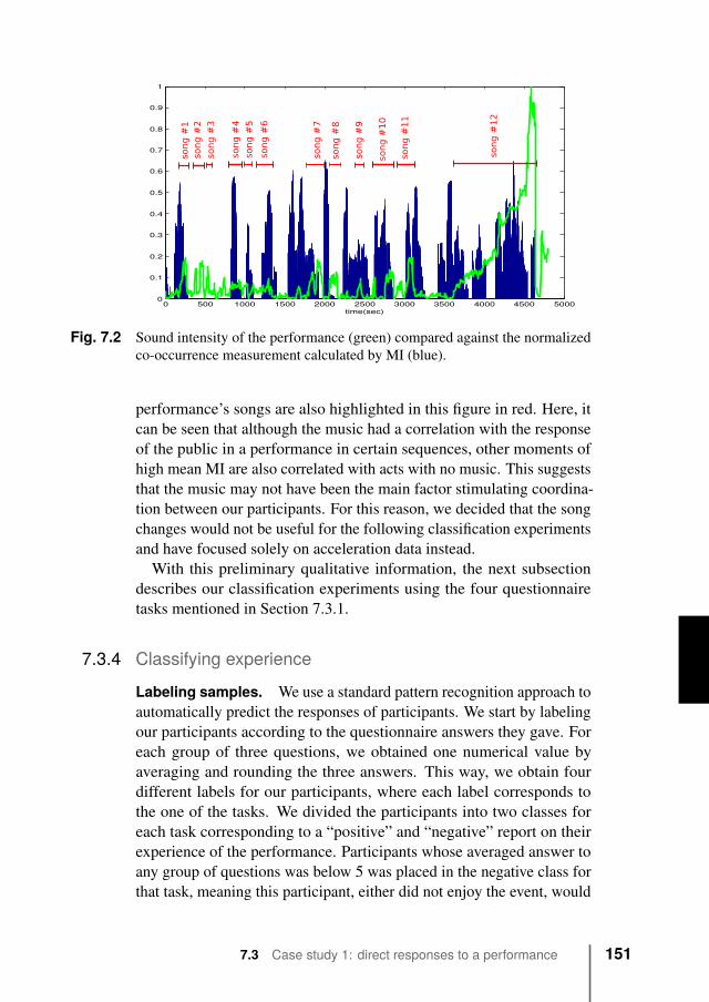
0 500 1000 1500 2000 2500 3000 3500 4000 4500 50000

0.1

0.2

0.3

0.4

0.5

0.6

0.7

0.8

0.9

1

time(sec)

son

g #

1so

ng

#2

son

g #

3

son

g #

4

song

#5

son

g #

6

son

g #

7

son

g #

8

son

g #

9

son

g #

10

song

#1

1

son

g #

12

Fig. 7.2 Sound intensity of the performance (green) compared against the normalizedco-occurrence measurement calculated by MI (blue).

performance’s songs are also highlighted in this figure in red. Here, itcan be seen that although the music had a correlation with the responseof the public in a performance in certain sequences, other moments ofhigh mean MI are also correlated with acts with no music. This suggeststhat the music may not have been the main factor stimulating coordina-tion between our participants. For this reason, we decided that the songchanges would not be useful for the following classification experimentsand have focused solely on acceleration data instead.

With this preliminary qualitative information, the next subsectiondescribes our classification experiments using the four questionnairetasks mentioned in Section 7.3.1.

7.3.4 Classifying experience

Labeling samples. We use a standard pattern recognition approach toautomatically predict the responses of participants. We start by labelingour participants according to the questionnaire answers they gave. Foreach group of three questions, we obtained one numerical value byaveraging and rounding the three answers. This way, we obtain fourdifferent labels for our participants, where each label corresponds tothe one of the tasks. We divided the participants into two classes foreach task corresponding to a “positive” and “negative” report on theirexperience of the performance. Participants whose averaged answer toany group of questions was below 5 was placed in the negative class forthat task, meaning this participant, either did not enjoy the event, would


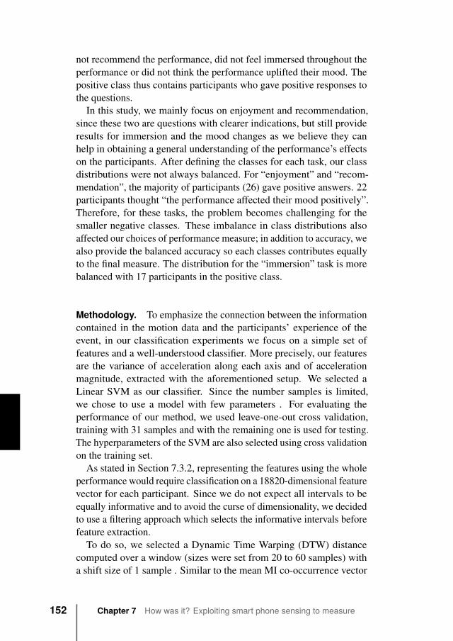
not recommend the performance, did not feel immersed throughout theperformance or did not think the performance uplifted their mood. Thepositive class thus contains participants who gave positive responses tothe questions.

In this study, we mainly focus on enjoyment and recommendation,since these two are questions with clearer indications, but still provideresults for immersion and the mood changes as we believe they canhelp in obtaining a general understanding of the performance’s effectson the participants. After defining the classes for each task, our classdistributions were not always balanced. For “enjoyment” and “recom-mendation”, the majority of participants (26) gave positive answers. 22participants thought “the performance affected their mood positively”.Therefore, for these tasks, the problem becomes challenging for thesmaller negative classes. These imbalance in class distributions alsoaffected our choices of performance measure; in addition to accuracy, wealso provide the balanced accuracy so each classes contributes equallyto the final measure. The distribution for the “immersion” task is morebalanced with 17 participants in the positive class.

Methodology. To emphasize the connection between the informationcontained in the motion data and the participants’ experience of theevent, in our classification experiments we focus on a simple set offeatures and a well-understood classifier. More precisely, our featuresare the variance of acceleration along each axis and of accelerationmagnitude, extracted with the aforementioned setup. We selected aLinear SVM as our classifier. Since the number samples is limited,we chose to use a model with few parameters . For evaluating theperformance of our method, we used leave-one-out cross validation,training with 31 samples and with the remaining one is used for testing.The hyperparameters of the SVM are also selected using cross validationon the training set.

As stated in Section 7.3.2, representing the features using the wholeperformance would require classification on a 18820-dimensional featurevector for each participant. Since we do not expect all intervals to beequally informative and to avoid the curse of dimensionality, we decidedto use a filtering approach which selects the informative intervals beforefeature extraction.

To do so, we selected a Dynamic Time Warping (DTW) distancecomputed over a window (sizes were set from 20 to 60 samples) witha shift size of 1 sample . Similar to the mean MI co-occurrence vector



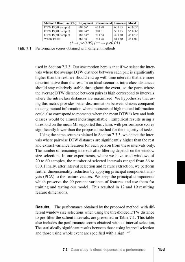
Method \ BAcc | Acc(%) Enjoyment Recommend Immerse MoodDTW IS(20 Sample) 60 | 66∗ 61 | 78 63 | 63 60 | 63∗

DTW IS(40 Sample) 90 | 94∗∗ 70 | 81 53 | 53 55 | 66∗

DTW IS(60 Sample) 78 | 84∗∗ 71 | 84 49 | 50 48 | 63∗

Whole Event 36 | 38 74 | 78 51 | 50 38 | 38(*→ p<0.05) (**→ p<0.01)

Tab. 7.1 Performance scores obtained with different methods

used in Section 7.3.3. Our assumption here is that if we select the inter-vals where the average DTW distance between each pair is significantlyhigher than the rest, we should end up with time intervals that are morediscriminative than the rest. In an ideal scenario, intra-class distancesshould stay relatively stable throughout the event, so the parts wherethe average DTW distance between pairs is high correspond to intervalswhere the intra-class distances are maximized. We hypothesize that us-ing this metric provides better discrimination between classes comparedto using mutual information where moments of high mutual informationcould also correspond to moments where the mean DTW is low and bothclasses would be almost indistinguishable . Empirical results using athreshold on the mean MI supported this claim, with performance scoressignificantly lower than the proposed method for the majority of tasks.

Using the same setup explained in Section 7.3.3, we detect the inter-vals where pairwise DTW distances are significantly higher than the restand extract variance features for each person from these intervals only.The number of remaining intervals after filtering depends on the windowsize selection. In our experiments, where we have used windows of20 to 60 samples, the number of selected intervals ranged from 86 to830. Finally, after interval selection and feature extraction, we performfurther dimensionality reduction by applying principal component anal-ysis (PCA) to the feature vectors. We keep the principal componentswhich preserve the 99 percent variance of features and use them fortraining and testing our model. This resulted in 12 and 19 resultingfeature dimensions.

Results. The performance obtained by the proposed method, with dif-ferent window size selections when using the thresholded DTW distanceto pre-filter the salient intervals, are presented in Table 7.1. This tablealso includes the performance scores obtained without interval selection.The statistically significant results between those using interval selectionand those using whole event are specified with a sign ’*’.


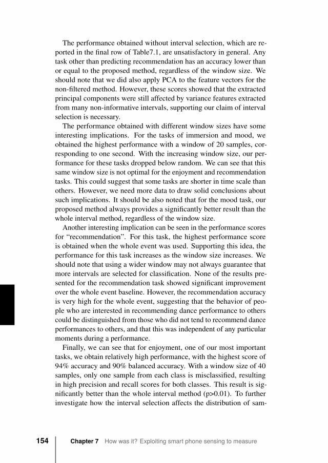
The performance obtained without interval selection, which are re-ported in the final row of Table7.1, are unsatisfactory in general. Anytask other than predicting recommendation has an accuracy lower thanor equal to the proposed method, regardless of the window size. Weshould note that we did also apply PCA to the feature vectors for thenon-filtered method. However, these scores showed that the extractedprincipal components were still affected by variance features extractedfrom many non-informative intervals, supporting our claim of intervalselection is necessary.

The performance obtained with different window sizes have someinteresting implications. For the tasks of immersion and mood, weobtained the highest performance with a window of 20 samples, cor-responding to one second. With the increasing window size, our per-formance for these tasks dropped below random. We can see that thissame window size is not optimal for the enjoyment and recommendationtasks. This could suggest that some tasks are shorter in time scale thanothers. However, we need more data to draw solid conclusions aboutsuch implications. It should be also noted that for the mood task, ourproposed method always provides a significantly better result than thewhole interval method, regardless of the window size.

Another interesting implication can be seen in the performance scoresfor “recommendation”. For this task, the highest performance scoreis obtained when the whole event was used. Supporting this idea, theperformance for this task increases as the window size increases. Weshould note that using a wider window may not always guarantee thatmore intervals are selected for classification. None of the results pre-sented for the recommendation task showed significant improvementover the whole event baseline. However, the recommendation accuracyis very high for the whole event, suggesting that the behavior of peo-ple who are interested in recommending dance performance to otherscould be distinguished from those who did not tend to recommend danceperformances to others, and that this was independent of any particularmoments during a performance.

Finally, we can see that for enjoyment, one of our most importanttasks, we obtain relatively high performance, with the highest score of94% accuracy and 90% balanced accuracy. With a window size of 40samples, only one sample from each class is misclassified, resultingin high precision and recall scores for both classes. This result is sig-nificantly better than the whole interval method (p>0.01). To furtherinvestigate how the interval selection affects the distribution of sam-



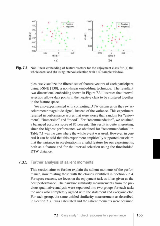
(a) (b)

Fig. 7.3 Non-linear embedding of feature vectors for the enjoyment class for (a) thewhole event and (b) using interval selection with a 40 sample window.

ples, we visualize the filtered set of feature vectors of each participantusing t-SNE [138], a non-linear embedding technique. The resultanttwo-dimensional embedding shown in Figure 7.3 illustrates that intervalselection allows data points in the negative class to be clustered togetherin the feature space.

We also experimented with computing DTW distances on the raw ac-celerometer magnitude signal, instead of the variance. This experimentresulted in performance scores that were worse than random for “enjoy-ment”, “immersion” and “mood”. For “recommendation”, we obtaineda balanced accuracy score of 85 percent. This result is quite interesting,since the highest performance we obtained for “recommendation” inTable 7.1 was the case where the whole event was used. However, in gen-eral it can be said that this experiment empirically supported our claimthat the variance in acceleration is a valid feature for our experiments,both as a feature and for the interval selection using the thresholdedDTW distance.

7.3.5 Further analysis of salient moments

This section aims to further explain the salient moments of the perfor-mance, now relating these with the classes identified in Section 7.3.4.For space reasons, we focus on the enjoyment task as it has given us thebest performance. The pairwise similarity measurements from the pre-vious qualitative analysis were separated into two groups for each task:the ones who completely agreed with the statement and everyone else.For each group, the same unified similarity measurement as describedin Section 7.3.3 was calculated and the salient moments were obtained


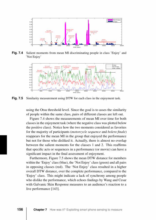
0 500 1000 1500 2000 2500 3000 3500 4000 4500 50000

0.1

0.2

0.3

0.4

0.5

0.6

0.7

0.8

0.9

1

time (sec)

Not EnjoyEnjoy

bolerosequence

resurrection sequence

motorcycle sequence

fun part(old lady)

maracassequence



3

1

1

3

8

8

5

Fig. 7.4 Salient moments from mean MI discriminating people in class ’Enjoy’ and’Not Enjoy’

bolerosequence

resurrection sequence motorcycle

sequence fun part(old lady)

maracassequence



0 500 1000 1500 2000 2500 3000 3500 4000 4500 50000

0.1

0.2

0.3

0.4

0.5

0.6

0.7

0.8

0.9

1

time (sec)

EnjoyNot EnjoyInter−class

Fig. 7.5 Similarity measurement using DTW for each class in the enjoyment task.

using the Otsu threshold level. Since the goal is to asses the similarityof people within the same class, pairs of different classes are left out.

Figure 7.4 shows the measurements of mean MI over time for bothclasses in the enjoyment task (where the negative class was plotted belowthe positive class). Notice how the two moments considered as favoritesfor the majority of participants (motorcycle sequence and bolero finale)reappears for the mean MI in the group that enjoyed the performancebut not for those who disliked it. Actually, there is almost no overlapbetween the salient moments for the classes 1 and 2. This reaffirmsthat specific acts or sequences in a performance (or movie) can have asignificant impact in the final assessment of enjoyment.

Furthermore, Figure 7.5 shows the mean DTW distance for memberswithin the ‘Enjoy’ class (blue), the ‘Not Enjoy’ class (green) and all pairsin opposing classes (red). The ‘Not Enjoy’ class resulted in a higheroverall DTW distance, over the complete performance, compared to the‘Enjoy’ class. This might indicate a lack of synchrony among peoplewho dislike the performance, which echoes findings by Wang and Cesarwith Galvanic Skin Response measures to an audience’s reaction to alive performance [143].



7.3.6 Identifying sitting neighbors

Knowing who is sitting close to whom is useful to study the spatio-temporal properties of audience response. Do neighboring individualstalk to each other at certain specific moments of the performance? Dopeople sitting close to each other react the same way (or at the sametime)? Does response (e.g., movement, emotion, mood) spread spatially,perhaps due to influence of neighbors? Yet, who is sitting where (orat least close to whom) is often unknown, as the audience is usuallyfree to choose where to seat and only rarely are seats assigned to thetickets by the theater. In this section we investigate whether we canleverage proximity data collected during the performance to identifywho is sitting close to whom.

Given that seats are placed such that all the audience is facing towardsthe same place, the stage, and that the proximity sensor worn on the chestyields face-to-face proximity detections, it is not obvious what kind ofinformation can be extracted from proximity detections collected duringthe performance. With sensors detecting other sensors at an angle ofaround 60 degrees towards the front, it is not clear how consistently theycan detect sensors worn by individuals sitting at the two sides, and howthe shielding effect of the body influences the detections of individualssitting in front or behind.

Furthermore, even assuming neighbors can be detected, it is unclearhow far they can be sensed (e.g., at how many rows or columns ofdistance), and how this relationship can be characterized, in particularconsidering no signal-strength (i.e., RSSI) is recorded by the sensors.

To start, one would assume that the closer two individuals sit, withinthe detection range of the sensor of 2-3 meters, the more frequently theirsensors will detect each other. First, given an individual u, we computethe number of times each ID of another sensor is detected during theperformance by the sensor worn by u, and we keep the top-K. Then,as we have recorded where volunteers were sitting in the theater inthe ground-truth, we generate ground-truth neighbors layout for eachindividual, and we compute precision and recall of the measurement, fora given K.

Precisely, assuming individual u is sitting at position ui, j, meaningat row i and column j, we compute from ground-truth the IDs of theindividuals (i) sitting at the sides (K = 2 individuals, which we call1-hop side neighbors, that is at positions ui, j+1 and ui, j−1) (ii) sittingin front and behind (K = 2 individuals, which we call frontal, that isat positions ui+1, j and ui+1, j), (iii) sitting at the sides of the 1-hop side


neighbors (K = 2 individuals, which we call 2-hop neighbors, that isat positions ui, j−2 and ui, j+2), and (iv) sitting at “diagonals” (K = 4individuals, that is at positions ui−1, j−1, ui−1, j+1, ui+1, j+1, and ui+1, j−1).We then compare these lists of IDs with those in the top-K lists.

Frontal and diagonal neighbors yield low recalls of 0.37 and 0.24respectively, while 1-hop neighbors yield precision of 0.62 and recallof 0.86. When we add also 2-hop neighbors, and hence using a valueof K = 4 (that is, we consider the 4 IDs appearing most frequently todetect 1-hop and 2-hop neighbors, 4 individuals in total), we obtain aprecision of 0.59 and a recall of 0.84. These results suggest that someof the neighbors detected for the 1-hop neighbors (with K = 2) are2-hop neighbors (lowering the precision), but 2-hop neighbors are notconsistently detected such that precision and recall are still similar withK = 4. The other source of error in precision in both cases are the raredetections of frontal and diagonal neighbors, which are not detectedconsistently but sometimes appear in the top-K list for some individuals.Moreover, the fact that 1-hop and 2-hop neighbors are mixed in thetop-K list makes it impossible to identify which is which based onfrequency (i.e., if 1-hop neighbors were detected more frequently than2-hop neighbors it would trivial).

Finally, one should notice that the K parameter is applied to all indi-viduals in the same way. However, for individuals who sit at the sidesof the theater, and hence have fewer 1-hop and 2-hop neighbors, thefixed value is not optimal. We investigated whether we could detectthese side cases by looking at the frequency distribution, but again wefound that there was no consistent way of classifying in which position aneighbor was sitting, given that neighbors are detected with a frequencynot directly connected to their position.

To conclude, the precision and recall values obtained when classifying1-hop and 2-hop neighbors show that it is possible to detect who is sittingat the sides of an individual (with some sampling of frontal and diagonalneighbors), and we plan to investigate further how signal-strength canhelp disambiguate between these classes.

7.4 Case study 2: impact of a performance on socialbehaviorSection 7.3 provided interesting insights into how the response to adance performance can be measured with pervasive sensing. However,while working with HD, we came across a different perspective on



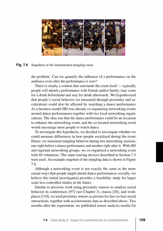
Fig. 7.6 Snapshots of the instrumented mingling room.

the problem. Can we quantify the influence of a performance on theaudience even after the performance is over?

There is clearly a context that surrounds the event itself — typically,people will attend a performance with friends and/or family, may comefor a drink beforehand and stay for drink afterwards. We hypothesizedthat people’s social behavior (as measured through proximity and ac-celeration) could also be affected by watching a dance performance.As a business model HD was already co-organizing networking eventsaround dance performances together with two local networking organi-zations. The idea was that the dance performance could be an occasionto enhance the networking event, and the co-located networking eventwould encourage more people to watch dance.

To investigate this hypothesis, we decided to investigate whether wecould measure differences in how people socialized during the event.Hence, we measured mingling behavior during two networking sessions,one right before a dance performance and another right after it. With HDand regional networking groups, we co-organised a networking eventwith 48 volunteers. The same sensing devices described in Section 7.3were used. An example snapshot of the mingling data is shown in Figure7.6.

Although a networking event is not exactly the same as the morecasual ways that people might attend dance performances socially, webelieve this initial investigation provides a feasibility study for largerscale less controlled studies in the future.

Similar to previous work using proximity sensors to analyze socialbehavior in conferences [97] (see Chapter 3), musea [26], and work-places [110], we used proximity sensors as proxies for face-to-face socialinteractions, together with accelerometer data as described above. Twomonths after the experiment, we published sensor analysis results for

7.4 Case study 2: impact of a performance on social behavior 159

the volunteers and asked them to answer a survey about their experienceof the dance performance and the networking event.

7.4.1 SetupTo measure whether people were interacting or not, we processed theproximity detections collected by the devices as follows. Because of theunreliability of the wireless medium, we used a density-based filteringtechnique to increase the sensitivity of the signal for detecting face-to-face proximity [98] (see Chapter 4). For each pair of individuals, wecomputed the intervals where pairs were continuously facing each other,formally [ti, t j] where ti is the timestamp of the first detection and t j isthe timestamp of the last detection of the interval. Because pairs canbe close for multiple non-overlapping time intervals during the samemeasurement, we computed multiple intervals for the same pair. Here,we refer to an interval of proximity between any pair as an interaction.For our experiments we considered only intervals of proximity longerthan 60s to indicate interactions.

7.4.2 ResultsSince some attendees did not attend the entire event, only the data from35 of the participants was available for analysis. We first hypothesizeda difference in the length or the number of interactions between thetwo sessions. For example, one could imagine that individuals wouldinteract in longer conversations, or with more people. In Figure 7.7(a)we present the distribution of the length of the interactions for the twosessions (from here on referred to as round 1 and round 2) across allthe individuals. In both rounds shorter interactions are predominant.Note that as drinks were served at the bar, during both rounds oftenindividuals left a conversation to fill their glass and went back rightafterwards to the same conversation, which would be measured as twodistinct interactions. No significant mean difference was seen betweenthe distribution in interaction length for the two rounds. In Figure 7.7(b)we present the distribution of the number of distinct interactions forround 1 and round 2 across all the individuals.

A second difference we hypothesized was in the size of conversationalgroups. For example, people could be engaged in conversations involv-ing more people, or conversely more one-to-one conversations, perhapsto discuss the content of the performance. We define a neighborhoodas the set of nodes a sensor a detects at a given moment in time, i.e.,



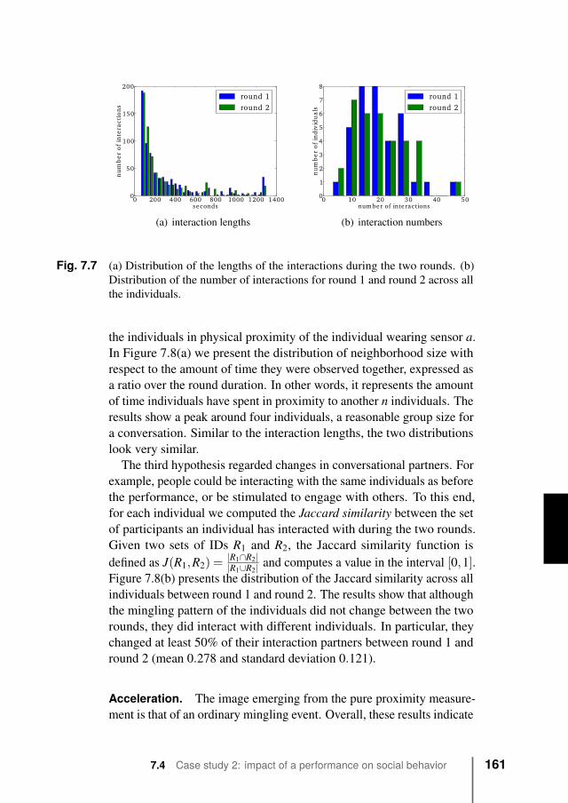
0 200 400 600 800 1000 1200 1400seconds

0

50

100

150

200

nu

mb

er

of

inte

ract

ion

s

round 1round 2

(a) interaction lengths

0 10 20 30 40 50number of inte ractions

0

1

2

3

4

5

6

7

8

nu

mb

er

of

ind

ivid

ua

ls

round 1round 2

(b) interaction numbers

Fig. 7.7 (a) Distribution of the lengths of the interactions during the two rounds. (b)Distribution of the number of interactions for round 1 and round 2 across allthe individuals.

the individuals in physical proximity of the individual wearing sensor a.In Figure 7.8(a) we present the distribution of neighborhood size withrespect to the amount of time they were observed together, expressed asa ratio over the round duration. In other words, it represents the amountof time individuals have spent in proximity to another n individuals. Theresults show a peak around four individuals, a reasonable group size fora conversation. Similar to the interaction lengths, the two distributionslook very similar.

The third hypothesis regarded changes in conversational partners. Forexample, people could be interacting with the same individuals as beforethe performance, or be stimulated to engage with others. To this end,for each individual we computed the Jaccard similarity between the setof participants an individual has interacted with during the two rounds.Given two sets of IDs R1 and R2, the Jaccard similarity function isdefined as J(R1,R2) =

|R1∩R2||R1∪R2| and computes a value in the interval [0,1].

Figure 7.8(b) presents the distribution of the Jaccard similarity across allindividuals between round 1 and round 2. The results show that althoughthe mingling pattern of the individuals did not change between the tworounds, they did interact with different individuals. In particular, theychanged at least 50% of their interaction partners between round 1 andround 2 (mean 0.278 and standard deviation 0.121).

Acceleration. The image emerging from the pure proximity measure-ment is that of an ordinary mingling event. Overall, these results indicate

7.4 Case study 2: impact of a performance on social behavior 161

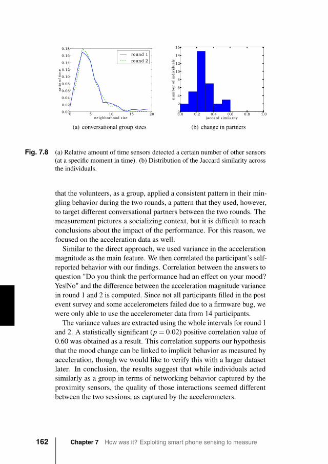
0 5 10 15 20ne ighborhood s ize

0.00

0.02

0.04

0.06

0.08

0.10

0.12

0.14

0.16

0.18

rati

o o

f ti

me

round 1round 2

(a) conversational group sizes

0.0 0.2 0.4 0.6 0.8 1.0jaccard s imilarity

0

2

4

6

8

10

12

14

16

nu

mb

er

of

ind

ivid

ua

ls

(b) change in partners

Fig. 7.8 (a) Relative amount of time sensors detected a certain number of other sensors(at a specific moment in time). (b) Distribution of the Jaccard similarity acrossthe individuals.

that the volunteers, as a group, applied a consistent pattern in their min-gling behavior during the two rounds, a pattern that they used, however,to target different conversational partners between the two rounds. Themeasurement pictures a socializing context, but it is difficult to reachconclusions about the impact of the performance. For this reason, wefocused on the acceleration data as well.

Similar to the direct approach, we used variance in the accelerationmagnitude as the main feature. We then correlated the participant’s self-reported behavior with our findings. Correlation between the answers toquestion "Do you think the performance had an effect on your mood?Yes|No" and the difference between the acceleration magnitude variancein round 1 and 2 is computed. Since not all participants filled in the postevent survey and some accelerometers failed due to a firmware bug, wewere only able to use the accelerometer data from 14 participants.

The variance values are extracted using the whole intervals for round 1and 2. A statistically significant (p = 0.02) positive correlation value of0.60 was obtained as a result. This correlation supports our hypothesisthat the mood change can be linked to implicit behavior as measured byacceleration, though we would like to verify this with a larger datasetlater. In conclusion, the results suggest that while individuals actedsimilarly as a group in terms of networking behavior captured by theproximity sensors, the quality of those interactions seemed differentbetween the two sessions, as captured by the accelerometers.



7.5 DiscussionWe have shown that by leveraging variance in the accelerometric signalit is possible to predict the response of the audience of a live danceperformance. One of the main contributions of such result is that itshows that information about the internal experience of the audience isembedded into something as simple as the small movements of seatedindividuals, if the whole involved crowd is taken into account. Whilevery promising, much more work needs to be done.

First, we have employed a blackbox supervised approach, where wepredicted the labels collected in the surveys. While labels could becollected for a subset of the audience and a semi-supervised approachcould be followed, it is not realistic to believe that one may require tocollect labels for each performance. Unsupervised approaches should beinvestigated further, and most importantly it is necessary to understandwhat fundamental and principal elements of the signal relate to whichmoods, emotions, and in general qualities of the response, and in whichway.

Second, we have focused on summarizing the whole experience witha label, whereas such method could, at least in principle, focus onspecific moments in time, hence applying different labels at differenttimes. Being able to characterize certain emotions and responses duringspecific moments of an event, and as early as possible, should enablemanagers to predict and act in a timely fashion, to avoid accidents andsteer a crowd towards safety and comfort.

Third, our volunteers were sitting during the performance, so moreresearch needs to be done to understand how to apply the methodol-ogy to different crowds and conditions where individuals are standing,moving or even dancing. The seated state has made things both simplerand harder at the same time. On the one hand, the range of ancillarybehaviors and actions have been minimized to the minimum, with theindividuals concentrating into following the dance performance at alltimes. On other hand, the range of movements have also been reduced tosmall and short movements, removing possibly more explicit reactionsthat are possible when an individual is free to move in space, and thatwould emerge, for example, in cases of emergency. Different events,conditions, and responses need to be investigated in the future.

Fourth, with the upcoming wave of wearables and sensors, accelerom-eters are just an example of sensors that can be used to collect data aboutcrowd response in a pervasive way. For example, new generations ofsmart watches already employ galvanic skin response sensors, which

7.5 Discussion 163

should yield information about arousal over time. We need to investigatewhich signal and sensor is more appropriate in which condition, andwhether fusing the sources of data can improve the picture we obtainout of the measurement.

Finally, regarding proximity, we have shown how spatio-temporalinformation can be used to understand who is seated close to whom andwho is talking to whom. However, we have only started to scratch thesurface of how spatio-temporal information, and in particular the tem-poral dimension, can be used to characterize the nature of the responseof the crowd, how it spreads, and how the different environmental andinternal factors influence the response.

7.6 ConclusionsWe have made a first investigation of how a seated audience’s percep-tion of a performance can be perceived and measured from their bodymovements using an accelerometer that exists typically in smart phones.We analyzed whether subtle and complex concepts such as “enjoyment”,“immersion”, an in improvement in mood as results of the performance,and whether participants would “recommend” dance in general, wouldbe reflected in body motion using a simple accelerometer hung aroundthe neck. Using the variance of the acceleration, we were already able topredict with 90% accuracy whether somebody enjoys the performance,which performed significantly above a random baseline.

Importantly, joint coordination in the variance in acceleration helpsto distinguish salient from non-salient moments, which lead to signif-icant improvements over using each person’s body movements fromthe entire performance period. As well as the obvious usefulness to theentertainment industry of such direct measurements of an audience’sreaction, we have also made a first attempt to measure the role that a liveperformance can have on the social behavior that precedes and follows it.Our experiments shows promise in enabling us to measure the implicitresponses of people while watching a live performance without the needfor more traditional sensing approaches using physiological or brainsignals.



8Conclusions

„Tell me and I forget, teach me and I mayremember, involve me and I learn.

— Benjamin Franklin

Spatio-temporal proximity data about individuals and objects can giveinsights about our social behavior and open a window in the digital worldover our life in the real world. Crowd managers report lack of situationawareness in their processes, and a desire for stronger ability to monitorand predict the behavior of a crowd, as well as to intervene to steerthe crowd to guarantee safety and comfort. Inexpensive miniaturizedproximity sensors, both mobile and fixed, can be used to collect suchspatio-temporal proximity information continuously, as the basis fortools to fulfill such needs.

Due to the unreliability of wireless communication, the data providedby the sensors needs to be filtered. Once the data is collected andfiltered, spatio-temporal proximity data can be modeled as a series ofso-called proximity graphs. By analyzing series of proximity graphs itis possible to identify and characterize different crowd behaviors, andbetter understand what is happening in a crowd. It is important forthese tools to operate in extreme cases, for example, of high densityand challenging environmental conditions, that is when such tools aremost needed. Moreover, spatio-temporal proximity information canbe used in cooperation with other sensor data to unveil higher-levelaspects of crowd behavior, including the more internal experience of theindividuals.

In this dissertation we have presented approaches to tackle all thesetasks, and that is how spatio-temporal proximity information can be col-lected, filtered, analyzed, and visualized to gain a better understandingof the behavior of a crowd.

165

8.1 Summary of contributionsIn particular, this dissertation makes the following contributions.

In Chapter 2, we studied current crowd management practices bymeans of ten interviews conducted with professionals managing someof the largest crowds in The Netherlands. Needs and requirements wereidentified, including the limitations of current approaches and technolo-gies. In particular, the interviewees reported a strong need for increasedsituation awareness, prediction, and intervention, positioning spatio-temporal aspects of crowd behavior, like density, flows, and congestions,at the top of their priorities. Recommendations were provided within theframework of a techno-social system for crowd management comprisingtwo feedback-control loops.

In Chapter 3, we dived into the definitions and properties of crowdtextures and proximity graphs. Examples of analyses to identify pedes-trian lanes, bottlenecks, and social groups were provided, along witha discussion about the importance of taking into account the contextaround a crowd, as well as advantages of instrumenting objects as wellas individuals with proximity sensors. A real-world use case was pre-sented, by identifying social groups within face-to-face proximity fromdata collected during an ICT conference.

In Chapter 4, we analyzed some of the sources of unreliability inmobile and fixed proximity sensing when applied to crowd monitoring.A filter with a few parameters, and a technique to choose good values forthem, was presented and evaluated both in simulation and in a numberof real-world experiments. The technique can double the sensitivity ofthe measurement, reconstructing nearly all missed proximity detectionsand ignoring spurious ones.

In Chapter 5, we focused on tracking an indoor crowd inside a mu-seum, studying in particular person-to-object face-to-face proximityrelationships. A pipeline of filters was presented, comprising a particlefilter adapted to directional sensing, together with a number of appli-cations to visualize, cluster, and predict the behavior of the museumvisitors, with data collected during a real-world 5-days experiment con-ducted at the CoBrA museum of Amsterdam. We also looked into theresults of a number of interviews and a focus group conducted withmuseum staff regarding the effectiveness of the visualizations.

In Chapter 6, we looked into an extension of the previous techniquethat takes into account also person-to-person proximity, to overcomelimitations caused by high densities. The technique was evaluated duringa large-scale experiment with nearly a thousand participants conducted at

166 Chapter 8 Conclusions

the NEMO museum, a particularly challenging setup due to the peculiarfeatures of the NEMO building. Together with the filtering pipeline, ananalysis to detect crowded events as well as flows between floors waspresented.

In Chapter 7, we studied how proximity sensors can be used togetherwith accelerometers to study the response of a crowd to a dance per-formance. An experiment was presented where audience behavior wastracked before, during, and after the performance, to try to identifythe response of the audience (e.g., enjoyment) by looking into the col-lective movements of the (seated) audience during the performance,and the differences in mingling behavior exhibited before and after theperformance.

8.2 Limitations and future researchTo conclude, we look at a number of possible directions for futureresearch, bootstrapped by some strengths and limitations of the workpresented in this dissertation.

Fine-grained crowddynamics. In Chapter 2 we have seen how crowdmanagers put increasing situation awareness about crowd dynamics andall behaviors with strong spatio-temporal nature at the top of their priori-ties. In Chapter 6 we have focused on detecting density spots and flows,but a more fine-grained approach, for example, like those described inChapter 3 to detect congestions and pedestrian lanes, should providemore detailed information about the properties of these crowd dynamics.While quantifying the number of people moving between floors at eachmoment helped unveiling the impact of the Chain Reaction event at theNEMO museum, understanding whether lanes form in these flows inan orderly fashion, as opposed to being perturbed and impeded by envi-ronmental factors, would enable crowd managers to react and influencethe design of the museum (e.g., the stairs, the positions of some exhibitsand divided walls, etc.). The information in the series of proximitygraphs should allow deeper analyses of the spatio-temporal relationshipsbetween the crowd members to identify and characterize even moreprecisely a wide range of existing crowd dynamics, and perhaps be thebasis for the discovery of new ones.

Integration into wearables and IoT. In this work, we have utilizeda number of custom-made devices that were either worn on the chest

8.2 Limitations and future research 167

hanging from the neck or as bracelet. For the former, we have exploitedthe shielding effect of the body for face-to-face proximity detection,while the latter provided a more uniform area of sensing around theindividual. We have also assumed that similar sensing capabilitiescould be obtained with smart phones via BLE, perhaps placed in ajacket pocket, or with a smart watch. These assumptions are not met,for example, when users put the phone in the trouser’s front or backpocket, or worse in a bag. It is important to find a consistent, reliable,and controllable way to shape the area of detection of the proximitysensor around the individual. A promising new area of research isthe integration of sensor and computing technology into clothing andtextiles, where “wires” are intermixed with standard clothing materialsin an imperceivable way, opening to a number of possible application forboth sensing, body-area networks, and interactive interfaces. Integratingproximity sensors, for example, inside of cloths like a jacket would allowto obtain a higher level of control about where the sensor is positionedwith respect to the body of the individual. A similar argument can bemade regarding the integration into objects and things. We interact ina different way with different objects like, for example, a fridge or abook, and different approaches need to be found to be able to capturethe nuances of each specific interaction type.

Sensing technology. BLE-like and in general radio-based proximitysensors are just examples of ways to detect proximity between two de-vices. Each specific technology comes with a different set of advantagesand disadvantages that can be exploited to obtain particular features forthe proximity sensor. For example, radio-based proximity sensing isknown to be influenced by the water and human bodies, but can passthrough certain types of materials that are used, for example, to buildwalls. This can make sensing co-location in dense environments par-ticularly challenging. On the other hand, light-based sensing tends tobe easier to confine within the boundaries of rooms and spaces. Fur-thermore, even remaining within radio-based proximity sensing, thechoice of frequency can have a large impact. For example, frequenciesaround the 2.4Ghz band such as those used by BLE and Zigbee tendto be particularly affected by water, whereas lower frequencies aroundthe 400Khz band, like those used by avalanche transceivers, are less af-fected by water but afford lower bandwidth. Further research is requiredinto mixing different proximity sensing technologies and signals at thesame time, to exploit the respective advantages and overcome the dis-


advantages (i.e., via multi-medium sensing). Finally, if the approachespresented in this dissertation were really to be deployed large-scale intoconsumer products like smart phones, more energy-efficient techniqueswould be necessary, as scanning BLE devices every second would drainthe battery of a smart phone within minutes.

Local and hybrid localization. Clearly, there are many points of over-lap between proximity-based positioning systems and indoor localiza-tions systems. One could consider in fact the system presented in Chap-ter 6 as a local localization system, where anchors act as landmarks forspecific local areas of interest (though we put less impact on computingcoordinates). The advantage is the ability to control accuracy in certainareas that are more challenging, for example, due to density or environ-mental conditions, by adding more anchors were needed. Upcomingextensions to BLE including angle-of-arrival information should allowbeacons to be utilized in the future as low-cost solutions for landmarkingas in traditional indoor localization systems where needed, or as posi-tioning anchors as proposed in this dissertation, hence forming hybridsolutions tailored to the specific needs of the user.

Feedback and steering of behavior. In this dissertation we have po-sitioned our work within a framework based on feedback-control loops.Large parts of our contributions focus on the sensing/input and process-ing/control steps of the loop, while we have implemented the feedbackstep through visualizations. At this time, there is little knowledge aboutthis latter step of the loop and research effort should be directed towardsresearch questions regarding, for example, (i) what information is re-quired by decisions makers at all levels (hence, including both managersand crowd members) and how it should be presented to them, (ii) whatintervention strategies are effective in which situations, (iii) how to pre-dict and avoid conditions instead of fixing them, as pro-active avoidanceis favorable to reaction, (iv) how technology can help to implementintervention strategies, for example, through actuators, interaction inter-faces, data sharing platforms etc. This work requires a multi-disciplinaryapproach involving the social and behavioral sciences, human-computerand user experience expertise, physics and mathematical modeling, andinformation-technology engineering. This is perhaps, at this point, themost challenging step in future work.

8.2 Limitations and future research 169

Applications beyond crowd behavior. In this work, we have fo-cused on crowd behavior as an instance of social behavior. However,with beacons deployed and detectable at large-scale in cities and build-ings, the smart devices we wear every day can act as HTTP/Web cookiesof the physical world. The number of applications that constant track-ing of our whereabouts enables are countless, with even more effectiveadvertising, to continue the analogy with HTTP/Web cookies, as themost clear example. Tracking proximity between individuals and ob-jects is at the basis of paradigms like the IoT and in general location-and context-aware computing, and one can easily imagine impact ontransport and logistics, product placement and recommendation in retail,support of social and entertainment events, payments. Clearly, a wideadoption of such monitoring and tracking applications requires devisingtechniques to maintain and respect the privacy of the users at all times,another important direction for future work.

Widermulti-sensor approach. As discussed in this dissertation, spatio-temporal proximity can only go so far to support the understanding of theinteractions between individuals (and objects). The realm of the studyof the quality of these interactions belongs to other type of sensors, op-erating as gateways to the internal experience of the individuals. Smartwatches, for example, are now provided with galvanic skin response sen-sors, heartbeat and blood pressure monitors, microphones and cameras,in addition to the sensors used to track activities, like accelerometersand gyroscopes. The value of the data provided by these sensors goesbeyond the monitoring of health levels. As shown in Chapter 7, thisdata contains information about the response of the individuals, andproximity information can act as the foundations to collect informationabout the context in which the individual is embedded during thoseresponses tracked by the other sensors. Future research is required toidentify which sensor is most effective in which context, perhaps alsoin conjunction with activity monitoring sensors that further enhance thecontext recognition capabilities of our devices. Finally, the informationthey provide can be fused together, including that of other individuals,to finally provide more complete and aware support.


Bibliography

[1] Nedal Ababneh. „Radio irregularity problem in wireless sensor networks:New experimental results“. In: Sarnoff Symposium, 2009. SARNOFF’09.IEEE. IEEE. 2009, pp. 1–5 (cit. on pp. 70, 92).

[2] JL Abbott and Morgan W Geddie. „Event and venue management:Minimizing liability through effective crowd management techniques“.In: Event Management 6.4 (2000), pp. 259–270 (cit. on p. 12).

[3] Norman Abramson. „The throughput of packet broadcasting channels“.In: IEEE Transactions on Communications 25.1 (1977), pp. 117–128(cit. on p. 69).

[4] S Adler, S Schmitt, Y Yang, Y Zhao, and M Kyas. Fubloc: Accuraterange-based indoor localization and tracking. Tech. rep. Technical re-port, Microsoft Indoor Localization Competition, 2014 (cit. on p. 90).

[5] Rakesh Agrawal and Ramakrishnan Srikant. „Privacy-preserving datamining“. In: ACM Sigmod Record. Vol. 29. 2. ACM. 2000, pp. 439–450(cit. on p. 37).

[6] Nadav Aharony, Wei Pan, Cory Ip, Inas Khayal, and Alex Pentland.„Social fMRI: Investigating and shaping social mechanisms in the realworld“. In: Pervasive and Mobile Computing 7.6 (2011), pp. 643–659(cit. on p. 59).

[7] S Al Bosta. „Crowd management based on scientific research to preventcrowd panic and disasters“. In: Pedestrian and Evacuation Dynamics.Springer, 2011, pp. 741–746 (cit. on p. 13).

[8] Nils Aschenbruck, Raphael Ernst, Elmar Gerhards-Padilla, and MatthiasSchwamborn. „BonnMotion: a mobility scenario generation and analysistool“. In: Proceedings of the 3rd International ICST Conference onSimulation Tools and Techniques. ICST (Institute for Computer Sciences,Social-Informatics and Telecommunications Engineering). 2010, p. 51(cit. on p. 68).

171

[9] Ashwin Ashok, Chenren Xu, Tam Vu, et al. „Bifocus: Using radio-optical beacons for an augmented reality search application“. In: Pro-ceeding of the 11th annual international conference on Mobile systems,applications, and services. ACM. 2013, pp. 507–508 (cit. on p. 90).

[10] Eleana Asimakopoulou and Nik Bessis. „Buildings and crowds: Formingsmart cities for more effective disaster management“. In: InnovativeMobile and Internet Services in Ubiquitous Computing (IMIS), 2011Fifth International Conference on. IEEE. 2011, pp. 229–234 (cit. onp. 14).

[11] Louis Atallah and Guang-Zhong Yang. „The use of pervasive sensingfor behaviour profiling - a survey“. In: Pervasive and Mobile Computing5.5 (2009), pp. 447–464 (cit. on p. 13).

[12] Ling Bao and Stephen S Intille. „Activity recognition from user-annotatedacceleration data“. In: International Conference on Pervasive Comput-ing. Springer. 2004, pp. 1–17 (cit. on p. 146).

[13] Xuan Bao, Songchun Fan, Alexander Varshavsky, Kevin Li, and RomitRoy Choudhury. „Your reactions suggest you liked the movie: Automaticcontent rating via reaction sensing“. In: Proceedings of the 2013 ACMinternational joint conference on Pervasive and ubiquitous computing.ACM. 2013, pp. 197–206 (cit. on p. 147).

[14] Christian Beder and Martin Klepal. „Fingerprinting based localisationrevisited: A rigorous approach for comparing RSSI measurements cop-ing with missed access points and differing antenna attenuations“. In:Indoor Positioning and Indoor Navigation (IPIN), 2012 InternationalConference on. IEEE. 2012, pp. 1–7 (cit. on pp. 90, 125).

[15] Nicola Bellomo and Christian Dogbe. „On the modeling of traffic andcrowds: A survey of models, speculations, and perspectives“. In: SIAMreview 53.3 (2011), pp. 409–463 (cit. on pp. 13, 34).

[16] Lucy Bennett. „Patterns of listening through social media: online fanengagement with the live music experience“. In: Social Semiotics 22.5(2012), pp. 545–557 (cit. on p. 145).

[17] Richard Bentley, John A Hughes, David Randall, et al. „Ethnographically-informed systems design for air traffic control“. In: Proceedings of the1992 ACM conference on Computer-supported cooperative work. ACM.1992, pp. 123–129 (cit. on p. 14).

[18] Alexander E Berlonghi. „Understanding and planning for different spec-tator crowds“. In: Safety Science 18.4 (1995), pp. 239–247 (cit. on pp. 19,38).

172 Bibliography

[19] Ulf Blanke, Gerhard Troster, Tobias Franke, and Paul Lukowicz. „Cap-turing crowd dynamics at large scale events using participatory gps-localization“. In: Intelligent Sensors, Sensor Networks and InformationProcessing (ISSNIP), 2014 IEEE Ninth International Conference on.IEEE. 2014, pp. 1–7 (cit. on p. 35).

[20] Bettina Bläsing, Beatriz Calvo-Merino, Emily S Cross, et al. „Neu-rocognitive control in dance perception and performance“. In: Actapsychologica 139.2 (2012), pp. 300–308 (cit. on p. 145).

[21] Alan S Brown and Jennifer L Novak. Assessing the intrinsic impacts of alive performance. WolfBrown San Francisco, CA, 2007 (cit. on p. 145).

[22] Erich Bruns, Benjamin Brombach, Thomas Zeidler, and Oliver Bimber.„Enabling mobile phones to support large-scale museum guidance“. In:IEEE multimedia 14.2 (2007), pp. 16–25 (cit. on pp. 91, 125).

[23] Tung X Bui and Siva R Sankaran. „Design considerations for a virtualinformation center for humanitarian assistance/disaster relief using work-flow modeling“. In: Decision support systems 31.2 (2001), pp. 165–179(cit. on p. 14).

[24] Beatriz Calvo-Merino, Corinne Jola, Daniel E Glaser, and Patrick Hag-gard. „Towards a sensorimotor aesthetics of performing art“. In: Con-sciousness and cognition 17.3 (2008), pp. 911–922 (cit. on p. 145).

[25] Marco Cattani, Marco Zuniga, Andreas Loukas, and Koen Langendoen.„Lightweight neighborhood cardinality estimation in dynamic wirelessnetworks“. In: Proceedings of the 13th international symposium onInformation processing in sensor networks. IEEE Press. 2014, pp. 179–189 (cit. on p. 33).

[26] Ciro Cattuto, Wouter Van den Broeck, Alain Barrat, et al. „Dynamics ofperson-to-person interactions from distributed RFID sensor networks“.In: PloS one 5.7 (2010), e11596 (cit. on p. 159).

[27] R Challenger, CW Clegg, and MA Robinson. „Understanding crowdbehaviours, Tech. rep“. In: Understanding Crowd Behaviours (Crown,2009) (2009), pp. 1–326 (cit. on p. 34).

[28] Rose Challenger and Chris W Clegg. „Crowd disasters: a socio-technicalsystems perspective“. In: Contemporary Social Science 6.3 (2011),pp. 343–360 (cit. on p. 12).

[29] W Challenger, WC Clegg, and AM Robinson. „Understanding crowdbehaviours: Guidance and lessons identified“. In: UK Cabinet Office(2009) (cit. on pp. 11, 13, 38).

[30] Albert Cherns. „Principles of sociotechnical design revisted“. In: Humanrelations 40.3 (1987), pp. 153–161 (cit. on p. 14).

Bibliography 173

[31] Albert Cherns. „The Principles of Sociotechnical Design1“. In: Humanrelations 29.8 (1976), pp. 783–792 (cit. on p. 14).

[32] Tanzeem Choudhury and Alex Pentland. „Sensing and modeling humannetworks using the sociometer“. In: interactions 5 (2003), p. 6 (cit. onpp. 42, 48, 80).

[33] Cinimodstudio. Peru national football stadium. http://cinimodstudio.com/project/peru-national-football-stadium/. 2011(cit. on p. 13).

[34] Chris Clegg and Craig Shepherd. „’The biggest computer programme inthe world ever!’: time for a change in mindset?“ In: Journal of Informa-tion Technology 22.3 (2007), pp. 212–221 (cit. on p. 14).

[35] Chris W Clegg. „Sociotechnical principles for system design“. In: Ap-plied ergonomics 31.5 (2000), pp. 463–477 (cit. on p. 14).

[36] Claudine Conrado and Patrick de Oude. „Scenario-based reasoningand probabilistic models for decision support“. In: Information Fusion(FUSION), 2014 17th International Conference on. IEEE. 2014, pp. 1–9(cit. on p. 34).

[37] Lynne Cooke. „Assessing concurrent think-aloud protocol as a usabilitytest method: A technical communication approach“. In: ProfessionalCommunication, IEEE Transactions on 53.3 (2010) (cit. on p. 108).

[38] Emily S Cross, Louise Kirsch, Luca F Ticini, and Simone Schütz-Bosbach. „The impact of aesthetic evaluation and physical ability ondance perception“. In: Frontiers in human neuroscience 5 (2011) (cit. onp. 145).

[39] Fred D Davis, Richard P Bagozzi, and Paul R Warshaw. „User accep-tance of computer technology: a comparison of two theoretical models“.In: Management science 35.8 (1989), pp. 982–1003 (cit. on p. 36).

[40] Matthew C Davis, Rose Challenger, Dharshana NW Jayewardene, andChris W Clegg. „Advancing socio-technical systems thinking: A callfor bravery“. In: Applied ergonomics 45.2 (2014), pp. 171–180 (cit. onp. 14).

[41] JF Dickie. „Major crowd catastrophes“. In: Safety science 18.4 (1995),pp. 309–320 (cit. on p. 12).

[42] Eyal Dim and Tsvi Kuflik. „Automatic detection of social behavior ofmuseum visitor pairs“. In: ACM Transactions on Interactive IntelligentSystems (TiiS) 4.4 (2015), p. 17 (cit. on pp. 91, 125).

[43] Trinh Minh Tri Do and Daniel Gatica-Perez. „Human interaction discov-ery in smartphone proximity networks“. In: Personal and UbiquitousComputing 17.3 (2013), pp. 413–431 (cit. on p. 59).

174 Bibliography

http://cinimodstudio.com/project/peru-national-football-stadium/

http://cinimodstudio.com/project/peru-national-football-stadium/

[44] Matthew Dobson, Spyros Voulgaris, and Maarten van Steen. „Mergingultra-low duty cycle networks“. In: 2011 IEEE/IFIP 41st InternationalConference on Dependable Systems & Networks (DSN). IEEE. 2011,pp. 538–549 (cit. on pp. 53, 60, 68).

[45] Matthew Dobson, Spyros Voulgaris, and Maarten Van Steen. „Network-level synchronization in decentralized social ad-hoc networks“. In: Per-vasive Computing and Applications (ICPCA), 2010 5th InternationalConference on. IEEE. 2010, pp. 206–212 (cit. on pp. 60, 68).

[46] Charalampos Doukas, Ilias Maglogiannis, Philippos Tragas, DimitrisLiapis, and Gregory Yovanof. „Patient fall detection using support vectormachines“. In: IFIP International Conference on Artificial IntelligenceApplications and Innovations. Springer. 2007, pp. 147–156 (cit. onp. 146).

[47] J Drechsel and A Kimms. „Task force deployment for big events“. In:Safety science 46.9 (2008), pp. 1289–1305 (cit. on p. 36).

[48] Dorine C Duives, Winnie Daamen, and Serge P Hoogendoorn. „State-of-the-art crowd motion simulation models“. In: Transportation researchpart C: emerging technologies 37 (2013), pp. 193–209 (cit. on p. 13).

[49] John RG Dyer, Anders Johansson, Dirk Helbing, Iain D Couzin, andJens Krause. „Leadership, consensus decision making and collectivebehaviour in humans“. In: Philosophical Transactions of the RoyalSociety of London B: Biological Sciences 364.1518 (2009), pp. 781–789(cit. on pp. 42, 45).

[50] Nathan Eagle and Alex Sandy Pentland. „Reality mining: sensing com-plex social systems“. In: Personal and ubiquitous computing 10.4 (2006),pp. 255–268 (cit. on p. 59).

[51] Cameron Earl, Elizabeth Parker, Andrew Tatrai, Mike Capra, et al. „Influ-ences on crowd behaviour at outdoor music festivals“. In: EnvironmentalHealth 4.2 (2004), p. 55 (cit. on p. 12).

[52] Mica R Endsley. „Toward a theory of situation awareness in dynamicsystems“. In: Human Factors: The Journal of the Human Factors andErgonomics Society 37.1 (1995), pp. 32–64 (cit. on p. 29).

[53] Gwenn Englebienne and Hayley Hung. „Mining for motivation: using asingle wearable accelerometer to detect people’s interests“. In: Proceed-ings of the 2nd ACM international workshop on Interactive multimediaon mobile and portable devices. ACM. 2012, pp. 23–26 (cit. on p. 146).

[54] Zeki Erkin, Jie Li, Arnold POS Vermeeren, and Huib de Ridder. „Privacy-Preserving Emotion Detection for Crowd Management“. In: Active Me-dia Technology. Springer, 2014, pp. 359–370 (cit. on p. 37).

Bibliography 175

[55] Martin Ester, Hans-Peter Kriegel, Jörg Sander, Xiaowei Xu, et al. „Adensity-based algorithm for discovering clusters in large spatial databaseswith noise.“ In: Kdd. Vol. 96. 34. 1996, pp. 226–231 (cit. on pp. 64, 95).

[56] Frédéric Evennou, François Marx, and Emil Novakov. „Map-aided in-door mobile positioning system using particle filter“. In: IEEE WirelessCommunications and Networking Conference, 2005. Vol. 4. IEEE. 2005,pp. 2490–2494 (cit. on pp. 93, 128).

[57] Z Fang, SM Lo, and JA Lu. „On the relationship between crowd densityand movement velocity“. In: Fire Safety Journal 38.3 (2003), pp. 271–283 (cit. on p. 29).

[58] Julien Fleureau, Philippe Guillotel, and Izabela Orlac. „Affective bench-marking of movies based on the physiological responses of a real audi-ence“. In: Affective Computing and Intelligent Interaction (ACII), 2013Humaine Association Conference on. IEEE. 2013, pp. 73–78 (cit. onp. 146).

[59] Behaviour in FTRE. „Human behaviour in fire: The development andmaturity of a scholarly study area“. In: Fire Mater 23 (1999), pp. 249–253 (cit. on p. 35).

[60] Raghu K Ganti, Fan Ye, and Hui Lei. „Mobile crowdsensing: currentstate and future challenges“. In: Communications Magazine, IEEE 49.11(2011), pp. 32–39 (cit. on p. 14).

[61] Raghu K Ganti, Nam Pham, Yu-En Tsai, and Tarek F Abdelzaher.„PoolView: stream privacy for grassroots participatory sensing“. In:Proceedings of the 6th ACM conference on Embedded network sensorsystems. ACM. 2008, pp. 281–294 (cit. on p. 37).

[62] Rafael C Gonzalez and Richard E Woods. „Digital image processing“.In: Nueva Jersey (2008) (cit. on p. 150).

[63] Fredrik Gustafsson, Fredrik Gunnarsson, Niclas Bergman, et al. „Particlefilters for positioning, navigation, and tracking“. In: IEEE Transactionson signal processing 50.2 (2002), pp. 425–437 (cit. on pp. 93, 128).

[64] S Gwynne, ER Galea, M Owen, Peter J Lawrence, L Filippidis, et al. „Areview of the methodologies used in evacuation modelling“. In: Fire andMaterials 23.6 (1999), pp. 383–388 (cit. on pp. 34, 35).

[65] Health and Safety Executive. „Managing Crowds Safely, A guide fororganisers at events and venues“. In: HSE books, 2014 (cit. on pp. 13,35, 38).

[66] Dirk Helbing and Anders Johansson. Pedestrian, crowd and evacuationdynamics. Springer, 2011 (cit. on p. 43).

176 Bibliography

[67] Dirk Helbing and Peter Molnar. „Social force model for pedestriandynamics“. In: Physical review E 51.5 (1995), p. 4282 (cit. on p. 13).

[68] Xiaoyan Hong, Mario Gerla, Guangyu Pei, and Ching-Chuan Chiang.„A group mobility model for ad hoc wireless networks“. In: Proceedingsof the 2nd ACM international workshop on Modeling, analysis andsimulation of wireless and mobile systems. ACM. 1999, pp. 53–60 (cit.on p. 68).

[69] Simon Hudson and Rupert Hudson. „Engaging with consumers usingsocial media: a case study of music festivals“. In: International Journalof Event and Festival Management 4.3 (2013), pp. 206–223 (cit. onp. 145).

[70] Pan Hui, Eiko Yoneki, Shu Yan Chan, and Jon Crowcroft. „Distributedcommunity detection in delay tolerant networks“. In: Proceedings of 2ndACM/IEEE international workshop on Mobility in the evolving internetarchitecture. ACM. 2007, p. 7 (cit. on p. 62).

[71] Hayley Hung, Gwenn Englebienne, and Jeroen Kools. „Classifying so-cial actions with a single accelerometer“. In: Proceedings of the 2013ACM international joint conference on Pervasive and ubiquitous com-puting. ACM. 2013, pp. 207–210 (cit. on p. 146).

[72] Hayley Hung, Gwenn Englebienne, and Laura Cabrera-Quiros. „Detect-ing conversing groups with a single worn accelerometer“. In: Proceed-ings of the 16th International Conference on Multimodal Interaction.ACM. 2014, pp. 84–91 (cit. on p. 146).

[73] Faisel T Illiyas, Shibu K Mani, AP Pradeepkumar, and Keshav Mohan.„Human stampedes during religious festivals: A comparative reviewof mass gathering emergencies in India“. In: International Journal ofDisaster Risk Reduction 5 (2013), pp. 10–18 (cit. on p. 14).

[74] Lorenzo Isella, Juliette Stehlé, Alain Barrat, et al. „What’s in a crowd?Analysis of face-to-face behavioral networks“. In: Journal of theoreticalbiology 271.1 (2011), pp. 166–180 (cit. on pp. 42, 48, 59, 80).

[75] Petra Isenberg, Niklas Elmqvist, Jean Scholtz, et al. „Collaborative visu-alization: definition, challenges, and research agenda“. In: InformationVisualization 10.4 (2011), pp. 310–326 (cit. on p. 35).

[76] Z Jiangy, W Xiy, Xiang-Yang Li, J Zhaoy, and J Hany. HiLoc: A TDoA-fingerprint hybrid indoor localization system. Tech. rep. Technical report,Microsoft Indoor Localization Competition, 2014 (cit. on p. 90).

[77] Naim Kapucu and Vener Garayev. „Collaborative decision-making inemergency and disaster management“. In: International Journal of Pub-lic Administration 34.6 (2011), pp. 366–375 (cit. on p. 36).

Bibliography 177

[78] Volker Kirchberg and Martin Tröndle. „The museum experience: Map-ping the experience of fine art“. In: Curator: The Museum Journal 58.2(2015), pp. 169–193 (cit. on pp. 91, 118, 125, 141).

[79] Mikkel Baun Kjærgaard, Martin Wirz, Daniel Roggen, and GerhardTröster. „Mobile sensing of pedestrian flocks in indoor environmentsusing wifi signals“. In: Pervasive Computing and Communications (Per-Com), 2012 IEEE International Conference on. IEEE. 2012, pp. 95–102(cit. on p. 59).

[80] Andreas Köpke, Michael Swigulski, Karl Wessel, et al. „Simulatingwireless and mobile networks in OMNeT++ the MiXiM vision“. In:Proceedings of the 1st international conference on Simulation tools andtechniques for communications, networks and systems & workshops.ICST (Institute for Computer Sciences, Social-Informatics and Telecom-munications Engineering). 2008, p. 71 (cit. on p. 70).

[81] Barbara Krausz and Christian Bauckhage. „Loveparade 2010: Automaticvideo analysis of a crowd disaster“. In: Computer Vision and ImageUnderstanding 116.3 (2012), pp. 307–319 (cit. on p. 125).

[82] Tsvi Kuflik, Zvi Boger, and Massimo Zancanaro. „Analysis and pre-diction of museum visitors’ behavioral pattern types“. In: UbiquitousDisplay Environments. Springer, 2012, pp. 161–176 (cit. on p. 84).

[83] Jennifer R Kwapisz, Gary M Weiss, and Samuel A Moore. „Activityrecognition using cell phone accelerometers“. In: ACM SigKDD Explo-rations Newsletter 12.2 (2011), pp. 74–82 (cit. on pp. 13, 146).

[84] Nicholas D Lane, Emiliano Miluzzo, Hong Lu, et al. „A survey of mo-bile phone sensing“. In: Communications Magazine, IEEE 48.9 (2010),pp. 140–150 (cit. on p. 14).

[85] Joel Lanir, Peter Bak, and Tsvi Kuflik. „Visualizing Proximity-BasedSpatiotemporal Behavior of Museum Visitors using Tangram Diagrams“.In: Computer Graphics Forum. Vol. 33. 3. Wiley Online Library. 2014,pp. 261–270 (cit. on pp. 102, 124).

[86] Celine Latulipe, Erin A Carroll, and Danielle Lottridge. „Love, hate,arousal and engagement: exploring audience responses to performingarts“. In: Proceedings of the SIGCHI Conference on Human Factors inComputing Systems. ACM. 2011, pp. 1845–1854 (cit. on p. 146).

[87] Patrick Lazik and Anthony Rowe. „Indoor pseudo-ranging of mobiledevices using ultrasonic chirps“. In: Proceedings of the 10th ACM Con-ference on Embedded Network Sensor Systems. ACM. 2012, pp. 99–112(cit. on p. 90).

178 Bibliography

[88] Anna Leask, Ahmed Hassanien, and Philip C Rothschild. „Social mediause in sports and entertainment venues“. In: International Journal ofEvent and Festival Management 2.2 (2011), pp. 139–150 (cit. on p. 145).

[89] Nancy G Leveson. „Applying systems thinking to analyze and learnfrom events“. In: Safety Science 49.1 (2011), pp. 55–64 (cit. on p. 35).

[90] Chin-Lung Li, Christos Laoudias, George Larkou, et al. „Indoor geolo-cation on multi-sensor smartphones“. In: Proceeding of the 11th annualinternational conference on Mobile systems, applications, and services.ACM. 2013, pp. 503–504 (cit. on pp. 90, 125).

[91] Jie Li, Huib de Ridder, APOS Vermeeren, Claudine Conrado, and Clau-dio Martella. „Designing for crowd well-being: Current designs, strate-gies and future design suggestions“. In: IASDR 2013: Proceedings of the5th International Congress of International Association of Societies ofDesign Research" Consilience and Innovation in Design", Tokyo, Japan,26-30 August 2013. 2013 (cit. on p. 36).

[92] Konrad Lorincz, David J Malan, Thaddeus RF Fulford-Jones, et al.„Sensor networks for emergency response: challenges and opportunities“.In: Pervasive Computing, IEEE 3.4 (2004), pp. 16–23 (cit. on p. 14).

[93] Paul Luff and Christian Heath. „The collaborative production of com-puter commands in command and control“. In: International Journal ofHuman-Computer Studies 52.4 (2000), pp. 669–699 (cit. on p. 14).

[94] Dimitrios Lymberopoulos, Jie Liu, Xue Yang, et al. „A realistic evalua-tion and comparison of indoor location technologies: Experiences andlessons learned“. In: Proceedings of the 14th international conferenceon information processing in sensor networks. ACM. 2015, pp. 178–189(cit. on pp. 89, 125, 126).

[95] Wendy E Mackay, Anne-Laure Fayard, Laurent Frobert, and Lionel Mé-dini. „Reinventing the familiar: exploring an augmented reality designspace for air traffic control“. In: Proceedings of the SIGCHI conferenceon Human factors in computing systems. ACM Press/Addison-WesleyPublishing Co. 1998, pp. 558–565 (cit. on p. 14).

[96] Oded Maimon and Lior Rokach. Data mining and knowledge discoveryhandbook. Vol. 2. Springer, 2005 (cit. on p. 110).

[97] Claudio Martella, Maarten Van Steen, A Halteren, Claudine Conrado,and Jie Li. „Crowd textures as proximity graphs“. In: CommunicationsMagazine, IEEE 52.1 (2014), pp. 114–121 (cit. on pp. 13, 61, 91, 141,159).

Bibliography 179

[98] Claudio Martella, Matthew Dobson, Aart Van Halteren, and MaartenVan Steen. „From proximity sensing to spatio-temporal social graphs“.In: Pervasive Computing and Communications (PerCom), 2014 IEEEInternational Conference on. IEEE. 2014, pp. 78–87 (cit. on pp. 54, 95,97, 131, 160).

[99] Claudio Martella, Ekin Gedik, Laura Cabrera-Quiros, Gwenn Englebi-enne, and Hayley Hung. „How Was It?: Exploiting Smartphone Sensingto Measure Implicit Audience Responses to Live Performances“. In:Proceedings of the 23rd ACM international conference on Multimedia.ACM. 2015, pp. 201–210 (cit. on pp. 118, 141).

[100] Claudio Martella, Armando Miraglia, Marco Cattani, and Maarten vanSteen. „Leveraging proximity sensing to mine the behavior of museumvisitors“. In: 2016 IEEE International Conference on Pervasive Com-puting and Communications (PerCom). IEEE. 2016, pp. 1–9 (cit. onp. 130).

[101] Mauro Martino, Francesco Calabrese, Giusy Di Lorenzo, et al. „Oceanof information: fusing aggregate & individual dynamics for metropoli-tan analysis“. In: Proceedings of the 15th international conference onIntelligent user interfaces. ACM. 2010, pp. 357–360 (cit. on p. 35).

[102] Aleksandar Matic, Venet Osmani, Alban Maxhuni, and Oscar Mayora.„Multi-modal mobile sensing of social interactions“. In: 2012 6th Interna-tional Conference on Pervasive Computing Technologies for Healthcare(PervasiveHealth) and Workshops. IEEE. 2012, pp. 105–114 (cit. onp. 146).

[103] Ramin Mehran, Akira Oyama, and Mubarak Shah. „Abnormal crowdbehavior detection using social force model“. In: IEEE Conf. on Com-puter Vision and Pattern Recognition (CVPR). IEEE. 2009, pp. 935–942(cit. on p. 125).

[104] Eve Mitleton-Kelly, Ivan Deschenaux, Christian Maag, Matthew Fuller-ton, and Nihan Celikkaya. Enhancing Crowd Evacuation and TrafficManagement Through AmI Technologies: A Review of the Literature.Springer, 2013 (cit. on p. 14).

[105] M Nakatsuka, H Iwatani, and J Katto. „A study on passive crowd densityestimation using wireless sensors“. In: The 4th Intl. Conf. on MobileComputing and Ubiquitous Networking (ICMU 2008). Citeseer. 2008(cit. on p. 126).

[106] Heather L O’Brien and Elaine G Toms. „The development and evaluationof a survey to measure user engagement“. In: Journal of the AmericanSociety for Information Science and Technology 61.1 (2010), pp. 501–769 (cit. on p. 148).

180 Bibliography

[107] Sung Park, Ivo Locher, Andreas Savvides, et al. „Design of a wear-able sensor badge for smart kindergarten“. In: Wearable Computers,2002.(ISWC 2002). Proceedings. Sixth International Symposium on.IEEE. 2002, pp. 231–238 (cit. on p. 81).

[108] Neal Patwari, Joshua N Ash, Spyros Kyperountas, et al. „Locating thenodes: cooperative localization in wireless sensor networks“. In: SignalProcessing Magazine, IEEE 22.4 (2005), pp. 54–69 (cit. on p. 126).

[109] Guangyu Pei and Thomas R Henderson. „Validation of OFDM errorrate model in ns-3“. In: Boeing Research Technology (2010), pp. 1–15(cit. on p. 72).

[110] Alex Pentland, Tanzeem Choudhury, Nathan Eagle, and Push Singh.„Human dynamics: computation for organizations“. In: Pattern Recogni-tion Letters 26.4 (2005), pp. 503–511 (cit. on pp. 59, 159).

[111] Ronald W Perry. „Incident management systems in disaster manage-ment“. In: Disaster Prevention and Management: An International Jour-nal 12.5 (2003), pp. 405–412 (cit. on p. 14).

[112] John W Ratcliff and David E Metzener. „Pattern-matching-the gestaltapproach“. In: Dr Dobbs Journal 13.7 (1988), p. 46 (cit. on p. 98).

[113] Matthew Reason and Dee Reynolds. „Kinesthesia, empathy, and relatedpleasures: An inquiry into audience experiences of watching dance“. In:Dance Research Journal 42.02 (2010), pp. 491–775 (cit. on p. 145).

[114] Madhu C Reddy, Sharoda A Paul, Joanna Abraham, et al. „Challengesto effective crisis management: using information and communicationtechnologies to coordinate emergency medical services and emergencydepartment teams“. In: International journal of medical informatics 78.4(2009), pp. 259–269 (cit. on p. 14).

[115] Sasank Reddy, Min Mun, Jeff Burke, et al. „Using mobile phones todetermine transportation modes“. In: ACM Transactions on Sensor Net-works (TOSN) 6.2 (2010), p. 13 (cit. on p. 146).

[116] Jörg Reichardt and Stefan Bornholdt. „Statistical mechanics of commu-nity detection“. In: Physical Review E 74.1 (2006), p. 016110 (cit. onp. 53).

[117] Stephen Reicher. „The psychology of crowd dynamics“. In: Blackwellhandbook of social psychology: Group processes (2001), pp. 182–208(cit. on p. 13).

[118] Rönne Reimann, Arne Bestmann, and Mirjam Ernst. „Locating technol-ogy for AAL applications with direction finding and distance measure-ment by narrow bandwidth phase analysis“. In: International Compe-tition on Evaluating AAL Systems through Competitive Benchmarking.Springer. 2012, pp. 52–62 (cit. on pp. 90, 125).

Bibliography 181

[119] Craig W Reynolds. „Flocks, herds and schools: A distributed behavioralmodel“. In: ACM SIGGRAPH computer graphics 21.4 (1987), pp. 25–34(cit. on p. 45).

[120] Daniel Roggen, Martin Wirz, Gerhard Tröster, and Dirk Helbing. „Recog-nition of crowd behavior from mobile sensors with pattern analysis andgraph clustering methods“. In: Networks and Heterogeneous Media,(2011) (cit. on pp. 13, 41, 42, 54).

[121] Elizabeth B-N Sanders and Pieter Jan Stappers. Convivial toolbox: Gen-erative research for the front end of design. BIS, 2012 (cit. on p. 17).

[122] Johan Schubert and Robert Suzic. „Decision support for crowd control:Using genetic algorithms with simulation to learn control strategies“.In: Military Communications Conference, 2007. MILCOM 2007. IEEE.IEEE. 2007, pp. 1–7 (cit. on p. 36).

[123] Thomas Schubert, Frank Friedmann, and Holger Regenbrecht. „Theexperience of presence: Factor analytic insights“. In: Presence 10.3(2001), pp. 266–281 (cit. on p. 148).

[124] Eric WK See-To, Savvas Papagiannidis, and Vincent Cho. „User ex-perience on mobile video appreciation: How to engross users and toenhance their enjoyment in watching mobile video clips“. In: Technolog-ical Forecasting and Social Change 79.8 (2012), pp. 1484–1494 (cit. onp. 148).

[125] AA Siddiqui and SMV Gwynne. „Employing pedestrian observationsin engineering analysis“. In: Safety science 50.3 (2012), pp. 478–493(cit. on p. 13).

[126] Jonathan D Sime. „Crowd psychology and engineering“. In: Safetyscience 21.1 (1995), pp. 1–14 (cit. on p. 13).

[127] RA Smith. „Density, velocity and flow relationships for closely packedcrowds“. In: Safety science 18.4 (1995), pp. 321–327 (cit. on p. 25).

[128] Bi Song, Ricky J Sethi, and Amit K Roy-Chowdhury. „Wide areatracking in single and multiple views“. In: Visual Analysis of Humans.Springer, 2011, pp. 91–107 (cit. on p. 125).

[129] RJC Stanton and GK Wanless. „Pedestrian movement“. In: Safety sci-ence 18.4 (1995), pp. 291–300 (cit. on p. 25).

[130] Bernhard Steffen and Armin Seyfried. „Methods for measuring pedes-trian density, flow, speed and direction with minimal scatter“. In: PhysicaA: Statistical mechanics and its applications 389.9 (2010), pp. 1902–1910 (cit. on p. 125).

182 Bibliography

[131] Catherine Stevens, Heather Winskel, Clare Howell, et al. „Direct andindirect methods for measuring audience reactions to contemporarydance“. In: (2009) (cit. on p. 146).

[132] G Keith Still. „Crowd dynamics“. PhD thesis. University of Warwick,2000 (cit. on p. 13).

[133] Robert Strohmaier, Gerhard Sprung, Alexander Nischelwitzer, and San-dra Schadenbauer. „Using Visitor Flow Visualization to Improve VisitorExperience in Museums and Exhibitions“. In: (2015) (cit. on p. 124).

[134] Lucy Suchman. „Centers of coordination: A case and some themes“.In: Discourse, Tools and Reasoning. Springer, 1997, pp. 41–62 (cit. onp. 14).

[135] Latanya Sweeney. „k-anonymity: A model for protecting privacy“. In:International Journal of Uncertainty, Fuzziness and Knowledge-BasedSystems 10.05 (2002), pp. 557–570 (cit. on p. 37).

[136] Martin Tröndle, Steven Greenwood, Konrad Bitterli, and Karen van denBerg. „The effects of curatorial arrangements“. In: Museum Managementand Curatorship 29.2 (2014), pp. 140–173 (cit. on p. 105).

[137] USA Today. Providence theater experiments with ’tweet seats’. http://www.usatoday.com/story/tech/2013/01/27/theater-tweet-seats/1868693/. 2013 (cit. on p. 145).

[138] Laurens Van der Maaten and Geoffrey Hinton. „Visualizing Data usingt-SNE.“ In: Journal of Machine Learning Research 9.11 (2008) (cit. onp. 155).

[139] Fiammetta Venuti, Luca Bruno, and Nicola Bellomo. „Crowd dynamicson a moving platform: Mathematical modelling and application to livelyfootbridges“. In: Mathematical and Computer Modelling 45.3 (2007),pp. 252–269 (cit. on p. 13).

[140] Eliséo Véron and Martine Levasseur. Ethnographie de l’exposition:l’espace, le corps et le sens. Centre Georges Pompidou, Bibliothèquepublique d’information, 1989 (cit. on p. 84).

[141] Alessandro Vinciarelli, Maja Pantic, and Hervé Bourlard. „Social sig-nal processing: Survey of an emerging domain“. In: Image and VisionComputing 27.12 (2009), pp. 1743–1759 (cit. on p. 13).

[142] Spyros Voulgaris, Matthew Dobson, and Maarten Van Steen. „Decentral-ized Network-level Synchronization in Mobile Ad Hoc Networks“. In:ACM Transactions on Sensor Networks (TOSN) 12.1 (2016), p. 5 (cit. onpp. 87, 148).

Bibliography 183

http://www.usatoday.com/story/tech/2013/01/27/theater-tweet-seats/1868693/



[143] Chen Wang and Pablo Cesar. „Do we react in the same manner?: com-paring GSR patterns across scenarios“. In: Proceedings of the 8th NordicConference on Human-Computer Interaction: Fun, Fast, Foundational.ACM. 2014, pp. 501–510 (cit. on p. 156).

[144] Chen Wang, Erik N Geelhoed, Phil P Stenton, and Pablo Cesar. „Sensinga live audience“. In: Proceedings of the 32nd annual ACM conferenceon Human factors in computing systems. ACM. 2014, pp. 1909–1912(cit. on p. 146).

[145] Joe H Ward Jr. „Hierarchical grouping to optimize an objective function“.In: Journal of the American statistical association 58.301 (1963) (cit. onp. 110).

[146] Elias Weingartner, Hendrik Vom Lehn, and Klaus Wehrle. „A perfor-mance comparison of recent network simulators“. In: 2009 IEEE Inter-national Conference on Communications. IEEE. 2009, pp. 1–5 (cit. onp. 68).

[147] Ferdinanda Elfrida Hubertina Wijermans. Understanding crowd be-haviour: Simulating situated individuals. University of Groningen Gronin-gen, 2011 (cit. on pp. 13, 16).

[148] Nanda Wijermans, Claudine Conrado, Maarten van Steen, ClaudioMartella, and Jie Li. „A landscape of crowd-management support: Anintegrative approach“. In: Safety science 86 (2016), pp. 142–164 (cit. onpp. 11, 125, 141).

[149] Gillian Wilson. „Multimedia tour programme at tate modern“. In: Muse-ums and the Web. Vol. 3. 2004 (cit. on pp. 91, 125).

[150] Moe Z Win, Andrea Conti, Santiago Mazuelas, et al. „Network local-ization and navigation via cooperation“. In: Communications Magazine,IEEE 49.5 (2011), pp. 56–62 (cit. on p. 126).

[151] William E Winkler. „String Comparator Metrics and Enhanced DecisionRules in the Fellegi-Sunter Model of Record Linkage.“ In: (1990) (cit.on pp. 98, 110).

[152] Martin Wirz, Tobias Franke, Eve Mitleton-Kelly, et al. „Coenosense:A framework for real-time detection and visualization of collectivebehaviors in human crowds by tracking mobile devices“. In: Proceedingsof the European Conference on Complex Systems 2012. Springer. 2013,pp. 353–361 (cit. on p. 35).

[153] Martin Wirz, Daniel Roggen, and Gerhard Troster. „Decentralized de-tection of group formations from wearable acceleration sensors“. In:Computational Science and Engineering, 2009. CSE’09. InternationalConference on. Vol. 4. IEEE. 2009, pp. 952–959 (cit. on p. 13).

184 Bibliography

[154] Martin Wirz, Tobias Franke, Daniel Roggen, et al. „Inferring crowdconditions from pedestrians’ location traces for real-time crowd mon-itoring during city-scale mass gatherings“. In: Enabling Technologies:Infrastructure for Collaborative Enterprises (WETICE), 2012 IEEE 21stInternational Workshop on. IEEE. 2012, pp. 367–372 (cit. on p. 13).

[155] Martin Wirz, Daniel Roggen, and G Troster. „User acceptance studyof a mobile system for assistance during emergency situations at large-scale events“. In: Human-Centric Computing (HumanCom), 2010 3rdInternational Conference on. IEEE. 2010, pp. 1–6 (cit. on p. 35).

[156] Martin Wirz, Eve Mitleton-Kelly, Tobias Franke, et al. Using mobiletechnology and a participatory sensing approach for crowd monitoringand management during large-scale mass gatherings. Springer, 2013(cit. on p. 13).

[157] Henk Wymeersch, Jaime Lien, and Moe Z Win. „Cooperative localiza-tion in wireless networks“. In: Proceedings of the IEEE 97.2 (2009),pp. 427–450 (cit. on p. 126).

[158] Zhongyang Xiong, Ruotian Chen, Yufang Zhang, and Xuan Zhang.„Multi-density dbscan algorithm based on density levels partitioning“.In: Journal of Information and Computational Science 9.10 (2012),pp. 2739–2749 (cit. on p. 66).

[159] Kazuo Yano, Koji Ara, Norihiko Moriwaki, and Hiroyuki Kuriyama.„Measurement of human behavior: creating a society for discoveringopportunities“. In: Hitachi Review 58.4 (2009), p. 139 (cit. on pp. 59,80).

[160] Andrew C Yao. „Protocols for secure computations“. In: 2013 IEEE54th Annual Symposium on Foundations of Computer Science. IEEE.1982, pp. 160–164 (cit. on p. 37).

[161] S Yaseen, A Al-Habaibeh, D Su, and F Otham. „Real-time crowd densitymapping using a novel sensory fusion model of infrared and visualsystems“. In: Safety science 57 (2013), pp. 313–325 (cit. on pp. 13, 125).

[162] Yuji Yoshimura, Fabien Girardin, Juan Pablo Carrascal, Carlo Ratti, andJosep Blat. New tools for studying visitor behaviours in museums: a casestudy at the Louvre. Springer-Verlag, 2012 (cit. on pp. 91, 125).

[163] Yaoxuan Yuan, Jizhong Zhao, Chen Qiu, and Wei Xi. „Estimating crowddensity in an RF-based dynamic environment“. In: IEEE Sensors Journal13.10 (2013), pp. 3837–3845 (cit. on p. 126).

[164] Marco Zúñiga Zamalloa and Bhaskar Krishnamachari. „An analysisof unreliability and asymmetry in low-power wireless links“. In: ACMTransactions on Sensor Networks (TOSN) 3.2 (2007), p. 7 (cit. on p. 72).

Bibliography 185

[165] Nikos Zarboutis and Nicolas Marmaras. „Design of formative evacuationplans using agent-based simulation“. In: Safety Science 45.9 (2007),pp. 920–940 (cit. on p. 13).

[166] Beibei Zhan, Dorothy N Monekosso, Paolo Remagnino, Sergio A Ve-lastin, and Li-Qun Xu. „Crowd analysis: a survey“. In: Machine Visionand Applications 19.5-6 (2008), pp. 345–357 (cit. on pp. 13, 125).

[167] Sheng Zhang, Weihong Wang, James Ford, and Fillia Makedon. „Learn-ing from Incomplete Ratings Using Non-negative Matrix Factorization.“In: SDM. Vol. 6. SIAM. 2006, pp. 548–552 (cit. on p. 115).

[168] Tong Zhang, Jue Wang, Ping Liu, and Jing Hou. „Fall detection byembedding an accelerometer in cellphone and using KFD algorithm“.In: International Journal of Computer Science and Network Security6.10 (2006), pp. 277–284 (cit. on p. 146).

[169] Gang Zhou, Tian He, Sudha Krishnamurthy, and John A Stankovic. „Im-pact of radio irregularity on wireless sensor networks“. In: Proceedingsof the 2nd international conference on Mobile systems, applications,and services. ACM. 2004, pp. 125–138 (cit. on pp. 70, 92).

[170] Han Zou, Lihua Xie, Qing-Shan Jia, and Hengtao Wang. „Platform andalgorithm development for a rfid-based indoor positioning system“. In:Unmanned Systems 2.03 (2014), pp. 279–291 (cit. on p. 90).

186 Bibliography

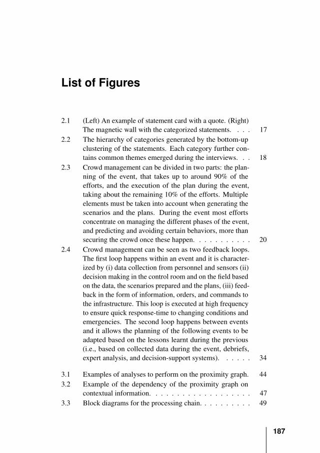
List of Figures

2.1 (Left) An example of statement card with a quote. (Right)The magnetic wall with the categorized statements. . . . 17

2.2 The hierarchy of categories generated by the bottom-upclustering of the statements. Each category further con-tains common themes emerged during the interviews. . . 18

2.3 Crowd management can be divided in two parts: the plan-ning of the event, that takes up to around 90% of theefforts, and the execution of the plan during the event,taking about the remaining 10% of the efforts. Multipleelements must be taken into account when generating thescenarios and the plans. During the event most effortsconcentrate on managing the different phases of the event,and predicting and avoiding certain behaviors, more thansecuring the crowd once these happen. . . . . . . . . . . 20

2.4 Crowd management can be seen as two feedback loops.The first loop happens within an event and it is character-ized by (i) data collection from personnel and sensors (ii)decision making in the control room and on the field basedon the data, the scenarios prepared and the plans, (iii) feed-back in the form of information, orders, and commands tothe infrastructure. This loop is executed at high frequencyto ensure quick response-time to changing conditions andemergencies. The second loop happens between eventsand it allows the planning of the following events to beadapted based on the lessons learnt during the previous(i.e., based on collected data during the event, debriefs,expert analysis, and decision-support systems). . . . . . 34

3.1 Examples of analyses to perform on the proximity graph. 443.2 Example of the dependency of the proximity graph on

contextual information. . . . . . . . . . . . . . . . . . . 473.3 Block diagrams for the processing chain. . . . . . . . . . 49

187

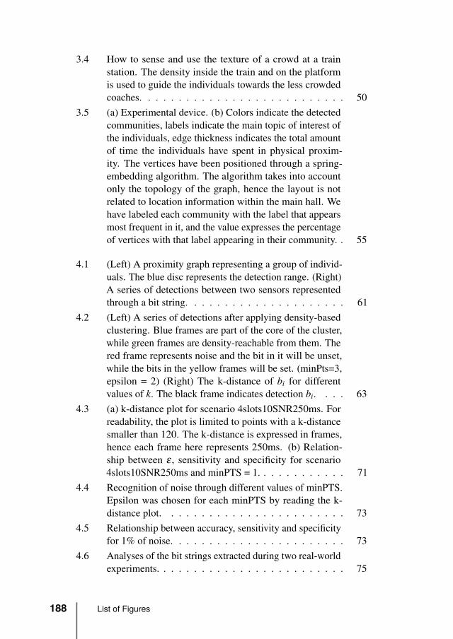
3.4 How to sense and use the texture of a crowd at a trainstation. The density inside the train and on the platformis used to guide the individuals towards the less crowdedcoaches. . . . . . . . . . . . . . . . . . . . . . . . . . . 50

3.5 (a) Experimental device. (b) Colors indicate the detectedcommunities, labels indicate the main topic of interest ofthe individuals, edge thickness indicates the total amountof time the individuals have spent in physical proxim-ity. The vertices have been positioned through a spring-embedding algorithm. The algorithm takes into accountonly the topology of the graph, hence the layout is notrelated to location information within the main hall. Wehave labeled each community with the label that appearsmost frequent in it, and the value expresses the percentageof vertices with that label appearing in their community. . 55

4.1 (Left) A proximity graph representing a group of individ-uals. The blue disc represents the detection range. (Right)A series of detections between two sensors representedthrough a bit string. . . . . . . . . . . . . . . . . . . . . 61

4.2 (Left) A series of detections after applying density-basedclustering. Blue frames are part of the core of the cluster,while green frames are density-reachable from them. Thered frame represents noise and the bit in it will be unset,while the bits in the yellow frames will be set. (minPts=3,epsilon = 2) (Right) The k-distance of bi for differentvalues of k. The black frame indicates detection bi. . . . 63

4.3 (a) k-distance plot for scenario 4slots10SNR250ms. Forreadability, the plot is limited to points with a k-distancesmaller than 120. The k-distance is expressed in frames,hence each frame here represents 250ms. (b) Relation-ship between ε , sensitivity and specificity for scenario4slots10SNR250ms and minPTS = 1. . . . . . . . . . . . 71

4.4 Recognition of noise through different values of minPTS.Epsilon was chosen for each minPTS by reading the k-distance plot. . . . . . . . . . . . . . . . . . . . . . . . 73

4.5 Relationship between accuracy, sensitivity and specificityfor 1% of noise. . . . . . . . . . . . . . . . . . . . . . . 73

4.6 Analyses of the bit strings extracted during two real-worldexperiments. . . . . . . . . . . . . . . . . . . . . . . . . 75

188 List of Figures

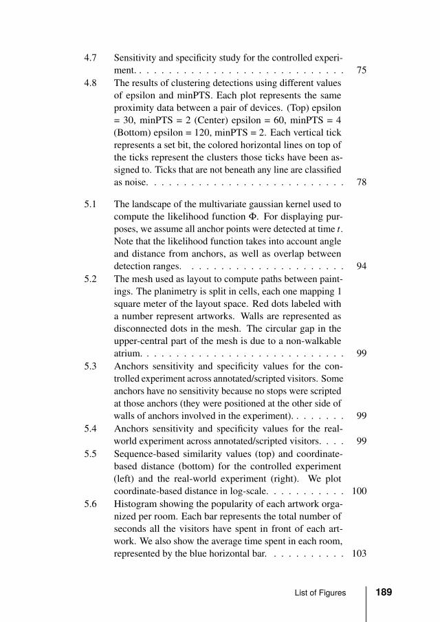
4.7 Sensitivity and specificity study for the controlled experi-ment. . . . . . . . . . . . . . . . . . . . . . . . . . . . . 75

4.8 The results of clustering detections using different valuesof epsilon and minPTS. Each plot represents the sameproximity data between a pair of devices. (Top) epsilon= 30, minPTS = 2 (Center) epsilon = 60, minPTS = 4(Bottom) epsilon = 120, minPTS = 2. Each vertical tickrepresents a set bit, the colored horizontal lines on top ofthe ticks represent the clusters those ticks have been as-signed to. Ticks that are not beneath any line are classifiedas noise. . . . . . . . . . . . . . . . . . . . . . . . . . . 78

5.1 The landscape of the multivariate gaussian kernel used tocompute the likelihood function Φ. For displaying pur-poses, we assume all anchor points were detected at time t.Note that the likelihood function takes into account angleand distance from anchors, as well as overlap betweendetection ranges. . . . . . . . . . . . . . . . . . . . . . 94

5.2 The mesh used as layout to compute paths between paint-ings. The planimetry is split in cells, each one mapping 1square meter of the layout space. Red dots labeled witha number represent artworks. Walls are represented asdisconnected dots in the mesh. The circular gap in theupper-central part of the mesh is due to a non-walkableatrium. . . . . . . . . . . . . . . . . . . . . . . . . . . . 99

5.3 Anchors sensitivity and specificity values for the con-trolled experiment across annotated/scripted visitors. Someanchors have no sensitivity because no stops were scriptedat those anchors (they were positioned at the other side ofwalls of anchors involved in the experiment). . . . . . . . 99

5.4 Anchors sensitivity and specificity values for the real-world experiment across annotated/scripted visitors. . . . 99

5.5 Sequence-based similarity values (top) and coordinate-based distance (bottom) for the controlled experiment(left) and the real-world experiment (right). We plotcoordinate-based distance in log-scale. . . . . . . . . . . 100

5.6 Histogram showing the popularity of each artwork orga-nized per room. Each bar represents the total number ofseconds all the visitors have spent in front of each art-work. We also show the average time spent in each room,represented by the blue horizontal bar. . . . . . . . . . . 103

List of Figures 189

5.7 Most frequent paths followed by the participants. Thethickness of each line is proportional to the frequency ofthe represented subpaths. . . . . . . . . . . . . . . . . . 104

5.8 Heatmap showing the amount of time spent in areas closeto artworks. Warmer colors are associated with areaswhere the participants have cumulatively spent most time. 107

5.9 The relationship between the most (red arrows, IDs 42,1, 15, 4, and 16) and the least (blue arrows, IDs 13, 8,27, 28, and 29) viewed artworks respectively and theirneighboring pieces. The pictures show the neighboringsources covering 50% of the total paths. . . . . . . . . . 107

5.10 Hierarchical agglomerative clustering of the visitor timedistribution vectors. At the center the distance matrixshows the distance between the vectors of all the visitors,while the dendograms show how the visitors have beengrouped together. . . . . . . . . . . . . . . . . . . . . . 111

5.11 The clustering algorithm identifies one small group (1-38,bottom) that spent time mostly in room 6, and anothermajor group (top) that is further clustered. Horizontalwhite lines show cluster divisions and black vertical linesroom divisions. . . . . . . . . . . . . . . . . . . . . . . 111

5.12 Visualization of the common paths chosen among thelargest group of visitors. . . . . . . . . . . . . . . . . . . 113

5.13 Visualization of the common paths chosen by the 10% ofvisitors that visited the exhibition starting from the end. . 113

5.14 (a) The original rating matrix generated from the rv vectorsand (b) the reconstruction of such matrix from lower-rankmatrices through Non-negative Matrix Factorization. . . 114

5.15 Distribution of prediction error across depending on theratio of reconstruction. . . . . . . . . . . . . . . . . . . 116

5.16 RMSE when choosing the test set with different criteriaand against a random predictor baseline. . . . . . . . . . 116

6.1 The map of the museum. The layout of the museumpresents challenging aspects, such as multiple stairs andelevators connecting the floors, an open-space nature aswell as the presence of closed rooms (e.g., auditoriums,labs, and theaters) and a series of balconies projecting overthe underlying floors. . . . . . . . . . . . . . . . . . . . 121

190 List of Figures

6.2 An example of the Chain Reaction event that periodicallyattracts dense crowds, sometimes from different floors.One can notice individuals around the event location, aswell as on the upper floors. . . . . . . . . . . . . . . . . 122

6.3 The problem can be thought as unfolding a lattice of nodeswith unknown location, leveraging the known locations ofthe anchors and the signal strength of mobile-to-mobileand mobile-to-anchor detections. . . . . . . . . . . . . . 127

6.4 Positioning accuracy during the controlled experiment atthe PoIs on the first floor and three additional “virtual”PoIs not instrumented with an anchor. We compare ourtechnique (not using here mobile-to-mobile proximity) toa technique that positions the visitor at the anchor withstrongest signal with and without a rolling window. Thecombined balanced accuracy, defined as the arithmeticmean between average sensitivity and specificity, for thetwo competing techniques and MONA (anchors only) were0.62, 0.69, and 0.81 respectively. . . . . . . . . . . . . . 133

6.5 Impact of neighbor bracelets around a visitor on the firstfloor. We added 5 more bracelets in the surrounding of thevisitor every 2 minutes of each stop. . . . . . . . . . . . 135

6.6 Positionings accuracy of our system with MONA and with-out it during the real-world experiment. Only PoIs 7, 9, 13,14, 16, 19 were instrumented with an anchor. The averagesensitivity was 0.68 and 0.77 respectively. . . . . . . . . 135

6.7 Number of individuals positioned at different PoIs overtime. (a) The number of visitors wearing a bracelet dur-ing the day (experiment participation was around 25%).(b) The Chain Reaction PoI. Events started at 11:15AM,12:15PM, 2:45PM, 3:15PM and 4:45PM for the durationof about 15 minutes. (c) The restaurant at the top floor.(d) An Auditorium open to the public only in 5 occasionsduring the day. . . . . . . . . . . . . . . . . . . . . . . . 137

6.8 Distribution of visitors across floors over time. As timepasses, the relative “popularity” of upper floors increases,with visitors moving up the building during their visit.Also, the Chain Reaction event plays a big role in the waypeople move across floors, attracting visitors from otherfloors. . . . . . . . . . . . . . . . . . . . . . . . . . . . 139

List of Figures 191

6.9 Flow of visitors from and to the first floor. One can noticethe influence of the Chain Reaction, as visitors tend toleave the floor by the stairs close-by the attraction afterthe event, and approach the floor from the other floorsbefore the event. . . . . . . . . . . . . . . . . . . . . . . 140

7.1 Mean co-occurrence measurement distance over time forall participants using Mutual Information (MI). Salientmoments are highlighted in red with number of appearance 150

7.2 Sound intensity of the performance (green) comparedagainst the normalized co-occurrence measurement calcu-lated by MI (blue). . . . . . . . . . . . . . . . . . . . . 151

7.3 Non-linear embedding of feature vectors for the enjoy-ment class for (a) the whole event and (b) using intervalselection with a 40 sample window. . . . . . . . . . . . . 155

7.4 Salient moments from mean MI discriminating people inclass ’Enjoy’ and ’Not Enjoy’ . . . . . . . . . . . . . . . 156

7.5 Similarity measurement using DTW for each class in theenjoyment task. . . . . . . . . . . . . . . . . . . . . . . 156

7.6 Snapshots of the instrumented mingling room. . . . . . . 1597.7 (a) Distribution of the lengths of the interactions during the

two rounds. (b) Distribution of the number of interactionsfor round 1 and round 2 across all the individuals. . . . . 161

7.8 (a) Relative amount of time sensors detected a certainnumber of other sensors (at a specific moment in time). (b)Distribution of the Jaccard similarity across the individuals.162

192 List of Figures

List of Tables

2.1 Description of the experts interviewed. . . . . . . . . . . 152.2 Current practices’ limitations and requirements for the

future. . . . . . . . . . . . . . . . . . . . . . . . . . . . 292.3 Overview of the impact of the envisioned techno-social

system on the crowd management operations emphasizedby the crowd managers as requiring aid from technology. 33

3.1 Sample statistics and results of the analysis. Additional17 participants were part of the organization and were notlabeled with one of the main tracks. . . . . . . . . . . . 53

4.1 Comparison of the results of the reconstruction of theproximity graph from raw data and with the two tech-niques. The results present the average outcome over the10 mobility patterns for each combination. For the density-based clustering technique, the chosen parameters wereminPT S = 1, and ε = 5,8,8,14 for each group of scenariorespectively. The values for ε were chosen by studyingthe k-distance plot for each group. For the window-basedsmoothing technique, the chosen parameters were ρ = 1,and n = 3,5,7,9 for each group of scenario respectively.The values for n were chosen experimentally to obtaincomparable results with respect to both sensitivity andspecificity. . . . . . . . . . . . . . . . . . . . . . . . . . 67

7.1 Performance scores obtained with different methods . . . 153

193

Summary

We are witnessing massive volumes of data about our behavior beingproduced and collected on a daily basis. This data comprises informationabout our multitude of activities online, including the World Wide Weband social networking and social media sites, as well a offline, recordedthrough the myriad of sensors installed in our smart phones and smartwatches. Effective modeling and analysis of such data opens the doorsto a number of applications and services that are more adaptive andpersonalized to the user, and to new paradigms like the Internet ofThings.

Spatio-temporal proximity is one of the signals that can be capturedwith existing technology like, for example, radio-based proximity sen-sors (e.g., Bluetooth Low Energy transceivers in modern smart phones).Spatio-temporal proximity data can be the foundation of a number ofanalyses of social behavior and in particular, the focus of this disserta-tion, of crowd behavior. Crowd behavior has a strong spatio-temporalnature, and it lends itself to be studied from this perspective. Further-more, a crowd is collective in nature, and the behavior of the membersof the crowd cannot be understood when looking at the individuals inisolation, but only when the behavior of all the members, together withthe relationships, is analyzed. We coined the term “crowd texture” to re-fer to the interleaved spatio-temporal relationships between the memberof a crowd that characterize specific crowd behaviors.

We started our work by interviewing ten crowd managers to under-stand the current crowd management practices and use of technology.We have found that crowd managers are interested in particular in meansof increasing situation awareness, prediction, and intervention, in par-ticular regarding movements and density variations in the crowd (e.g.,flows and congestions), but also higher level aspects such as mood, inparticular when conditions are critical. We have also found that crowdmanagers rely on technology only to a limited extent, as the current

195

existing solutions are found unreliable in most cases. Based on theseresults, we set as the main research question whether we can lever-age spatio-temporal proximity information collected through proximitysensors to gain a better understanding of the behavior of a crowd, tosupport the work of researchers and practitioners towards safer and morecomfortable crowds.

In this dissertation, we model spatio-temporal proximity as a seriesof proximity graphs, where each graph represents which entities werewithin a certain range of distance at a specific moment in time. In aproximity graph a vertex represents an entity while an edge representsa positive proximity relationship between two entities. By mining aseries of proximity graphs it is possible to identify and quantify differentcrowd behavior and dynamics, like pedestrian lanes, clogging, socialgroups, as well as group behavior. Together with the model, we proposea general approach to sense and collect the texture of a crowd thoughradio-based proximity sensors.

Due to the inherent limitations of wireless sensors networks andradio-based communication, proximity graphs collected with proximitysensors are often noisy and incomplete, meaning that proximity rela-tionships can be wrongly added or missing. Proximity graphs can befiltered to infer the missing relationships and remove the noisy ones. Inparticular, we present a novel filter based on a density-based clusteringalgorithm that identifies automatically intervals of proximity betweenentities in the data, and nearly doubles the accuracy of the measure-ment. We also present a solution to compute optimal parameters for thetechnique and we validate it both in simulation and through real-worldexperiments.

Once proximity data is collected and filtered, it can be analyzed toidentify group behavior and gain insight about the behavior of a crowd.We have deployed our infrastructure inside of the CoBrA museum ofAmsterdam to track the behavior of some of its visitors (who volunteeredto wear one of our sensors), by installing some proximity sensors atexhibits. Working together with the museum staff, we have produceda number of visualizations that helped the museum staff to better un-derstand the amount of time spent by the visitors at each exhibit andthe paths within the exhibition rooms followed by them, to name a fewexamples.

Crowd density is one of the characteristics crowd managers are mostinterested in, as it can be the cause (or fingerprint) of extreme anddangerous situations. Crowd density is also a major obstacle to radio-

196

based communication, hindering in particular proximity sensing systemsthat rely on long-range transmissions between wearable sensors andfixed infrastructure. This means that these solutions often fail in thevery conditions where they are most needed. We present a solution thatleverages mobile-to-mobile proximity sensing to overcome limitationsof mobile-to-fixed solutions when crowd density is high. We deployedour solution at the NEMO museum in Amsterdam, a museum locatedin a complex building characterized by a multi story open space thatis particularly challenging for radio-based communication. During ourexperiment, crowd density at peak was high, with more than 600 visitorswearing our sensor (and overall around 2400 visitors in the museum atthat moment). We show that crowd density can be leveraged to increasemeasurement accuracy as well as to gain insights about the behavior ofthe visitors.

Spatio-temporal proximity is an effective proxy for measuring crowdbehavior, yet it cannot be used to understand higher-level aspects ofcrowd behavior, which are important to study, for example, mood. Infact, other signals like galvanic skin response, audio and accelerationare more suitable to study the response and the inner experience ofthe members of the crowd. Still, spatio-temporal proximity can playan important role in these studies, as it can help the understandingof how the response of the crowd (e.g., mood and emotions) spreadspatio-temporally across the crowd. We have deployed our proximitysensing infrastructure together with accelerometers that we have used topredict the response of the audience of a dance performance. We showthat by measuring proximity and movement of the audience during theperformance as well as during mingling sessions before and after theperformance, we can predict the enjoyment of the audience.

The work presented in this dissertation shows promising results of theapplication of pervasive and ubiquitous proximity sensing to the studyof social behavior that open a number of new research directions forfuture work.

197

Samenvatting

We zien dat er tegenwoordig op dagelijkse basis enorm veel gegevensover ons gedrag verzameld wordt. Dit zijn gegevens over onze on-line activiteiten, zoals surfgedrag, sociale netwerken en sociale mediasites, maar ook offline activiteiten, die door allerlei sensoren wordtopgenomen in onze telefoons en horloges. We kunnen applicaties endiensten beter op de gebruiker afgestemd maken als we deze gegevensgoed kunnen modelleren en analyseren. Dan kan ook het meeste uitnieuwe werkwijzen zoals het Internet of Things gehaald worden.

Nabijheid in tijd en ruimte is een van de signalen die met huidigetechnologie al opgenomen kunnen worden, zoals radio-gebaseerde nabi-jheidssensoren (bijv. Bluetooth Low Energy radio chips in modernetelefoons). Analyse van deze nabijheids informatie kan de hoeksteenvormen van een aantal analyses van sociaal gedrag, en met name hetgedrag van een menigte. Dit is het aandachtsgebied van dit proefschrift.Het gedrag van mensenmassa’s kenmerkt zich door eigenschappen diezich in tijd en ruimte uitdrukken. Deze eigenschappen lenen zich goedvoor studie vanuit dit perspectief. Verder is een menigte van nature eengezamenlijk fenomeen. Gedrag van individuen in de menigte kan nietbegrepen worden door naar de geïsoleerde individuen te kijken, maaralleen door naar het gedrag van alle individuen en de relaties met elkaarte kijken en te analyseren. We stellen de term “menigte structuur” voorvoor het beschrijven van de relaties in tijd en ruimte tussen individuenin een menigte die specifiek gedrag in menigtes voortbrengt.

We zijn begonnen met tien menigte beheerders te ondervragen naarhuidige beheerstechnieken en technologie gebruik. We zijn erachtergekomen dat menigte beheerders met name geïnteresseerd zijn in hetverhogen van de situatie bewustheid, voorspelling, en interventie, metname wat betreft bewegingen en dichtheid variaties in de menigte (bijv.stromen en opstoppingen), maar ook hoger-niveau aspecten zoals stem-ming, voornamelijk wanneer omstandigheden kritiek zijn. We zijn er ook

199

achter gekomen dat menigte beheerders slechts in beperkte mate zich vantechnologie afhankelijk maken, omdat huidige oplossingen in de meestegevallen te onbetrouwbaar zijn gebleken. Hierop bouwend hebben weons de onderzoeksvraag gesteld: kunnen we door nabijheidssensorenopgevangen informatie, oftewel nabijheidsinformatie in ruimtelijke- entijds-zin, om beter begrip te krijgen van het gedrag van een menigte, omhet werk van onderzoekers en beoefenaars te ondersteunen om veiligereen prettigere menigtes te bewerkstelligen.

In dit proefschrift modelleren we nabijheid met een serie van nabi-jheidsgrafen, waarbij elke graaf weergeeft welke entiteiten zich op eenbepaald moment binnen een zekere afstand van elkaar bevonden. Ineen nabijheidsgraaf is een punt (of knoop) een entiteit, en een lijn (ofkant) een nabijheidsrelatie tussen twee entiteiten. We kunnen een aan-tal nabijheidsgrafen analyseren, en daarmee een verschillende gevallenvan menigte gedrag en dynamiek identificeren en kwantificeren. Voor-beelden zijn voetgangerspaden, opstoppingen, sociale groepen, en groeps-gedrag. Samen met dit model stellen we een algemene aanpak van hetmeten en verzamelen van de structuur van een menigte door middel vanradiosensoren voor.

Vanwege inherente beperkingen aan draadloze sensornetwerken en ra-diocommunicatie zijn nabijheidsgrafen die verzameld zijn met nabijhei-dssensoren niet compleet. Dit houdt in dat nabijheidsrelaties onterechtaanwezig zijn of onterecht afwezig zijn. Nabijheidsrelaties kunnen gefil-terd worden om de missende relaties aan te vullen en de onterechteweg te halen. We presenteren een automatisch filter dat gebaseerd isop een clustering algoritme dat automatisch intervallen van nabijheidtussen entiteiten identificeert in de metingen. Deze techniek maakt denauwkeurigheid van de meting bijna twee keer zo groot. We presenterenook een techniek om de optimale parameters voor de techniek te bereke-nen. Deze worden zowel door simulatie als door echte experimentensolide getoond.

Zodra nabijheidsdata gefilterd en verzameld is kan het geanalyseerdworden om groepsgedrag te vinden en inzicht te krijgen in het gedragvan een menigte. We hebben onze infrastructuur in het CoBrA museumvan Amsterdam uitgerold om het gedrag van een aantal van de bezoekerste volgen (die vrijwillig een van onze sensoren gedragen hebben), doorwat nabijheidssensoren bij tentoonstellingen te installeren. We hebbensamen met het personeel van het museum wat visualisaties gemaaktwaardoor het gedrag van de bezoekers beter begrepen kon worden - bij

200

voorbeeld hoe lang bezoekers bij elk onderdeel van de tentoonstellingstil hebben gestaan, en de paden die binnen de ruimtes gevolgd zijn.

Menigte dichtheid is een van de eigenschappen waar menigte be-heerders het meeste in geinteresseerd zijn, omdat het de aanleiding(of kenmerk) van extreme of gevaarlijke situaties kan zijn. Menigtedichtheid is ook een groot obstakel in radio-gebaseerde communicatie,met name omdat nabijheids detectie systemen gehinderd worden dieafhankelijk zijn van lange-afstandscommunicatie met vaste infrastruc-tuur. Dit betekent dat deze oplossingen vaak falen in precies die om-standigheden waarin ze het meest nodig zijn. We presenteren een oploss-ing die mobiel-naar-mobiel nabijheidsdetectie inzet om de beperkingenvan mobiel-naar-vaste oplossingen te overwinnen. We hebben onzeoplossing bij het NEMO museum in Amsterdam uitgerold, een museumdat in een complex gebouw gehuisvest is dat gekarakteriseerd wordtdoor een open ruimte van meerdere verdiepingen dat bij uitstek prob-lematisch is voor radiocommunicatie. Tijdens ons experiment was demenigte dichtheid op piekmomenten hoog, met meer dan 600 bezoekersdie onze sensor droegen (van een totaal van 2400 bezoekers in het mu-seum op dat moment). We laten zien dat menigte dichtheid juist ingezetkan worden om zowel meting nauwkeurigheid te verhogen als inzicht tekrijgen in het gedrag van de bezoekers.

Ruimte-tijds nabijheid is een effectief surrogaat voor het meten vanmenigte gedrag, maar het kan niet gebruikt worden om hoger-niveauaspecten van menigte gedrag te begrijpen, die ook belangrijk zijn om tebestuderen, zoals stemming. Andere metingen zoals elektrische weer-stand van de huid, audio, en acceleratie zijn bruikbaarder om de responsen innerlijke ervaring van de leden van de massa te bestuderen. Ruimte-tijds nabijheid kan echter toch een belangrijke rol spelen in deze studies,omdat het de reactie van de menigte (bijv. Stemming en emoties) en deruimte-tijds verspreiding door de massa heen kan helpen begrijpen. Wehebben onze nabijheids detectie infrastructuur samen met acceleratieme-ters uitgerold om de reactie van het publiek van een dansuitvoeringte voorspellen. We laten zien dat door nabijheid en beweging van hetpubliek zowel tijdens de uitvoering als tijdens de sociale interactie vooren na de uitvoering te meten, we de plezierbeleving van het publiekkunnen voorspellen.

Het werk dat in dit proefschrift wordt gepresenteerd laat veelbelovenderesultaten zien van de toepassing van alom aanwezige nabijheidsdetectieop de studie van sociaal gedrag dat een aantal nieuwe onderzoeksrichtin-gen voor verder onderzoekswerk opent.

201

Documents

Crowd Textures5ptFrom Sensing Proximity to Understanding ... dissertation.pdf · conduct research and write papers, and most importantly making it a lot of fun. The support I received