Embed Size (px)
Citation preview

Ann. Henri Poincare 13 (2012), 813–826c© 2011 Springer Basel AG
1424-0637/12/040813-14
published online November 3, 2011DOI 10.1007/s00023-011-0147-7 Annales Henri Poincare
Crossover to the KPZ Equation
Patrıcia Goncalves and Milton Jara
Abstract. We characterize the crossover regime to the KPZ equation fora class of one-dimensional weakly asymmetric exclusion processes. Thecrossover depends on the strength asymmetry an2−γ (a, γ > 0) and itoccurs at γ = 1/2. We show that the density field is a solution of anOrnstein-Uhlenbeck equation if γ ∈ (1/2, 1], while for γ = 1/2 it is anenergy solution of the KPZ equation. The corresponding crossover for thecurrent of particles is readily obtained.
1. Introduction
One-dimensional weakly asymmetric exclusion processes arise as simple mod-els for the growing of random interfaces. For those processes, the microscopicdynamics is given by stochastic lattice gases with hard core exclusion witha weak asymmetry to the right. The presence of a weak asymmetry breaksdown the detailed balance condition, which forces the system to exhibit a nontrivial behavior even in the stationary situation. Using renormalization grouptechniques, the dynamical scaling exponent has been established as z = 3/2and one of the challenging problems is to derive the limit distribution of thedensity and the current of particles [22].
For asymmetric exclusion processes, partial answers have been given inparticular settings as starting the system from the stationary state and fromspecific initial conditions. For these model, under a certain spatial shiftingand time speeding, the current of particles has Tracy–Widom distribution,see [11,15,23,24]. The Tracy–Widom distribution was initially obtained in thecontext of large N statistics of the largest eigenvalue of random matrices, buthas been recently obtained as the scaling limit of stochastic fields of randommodels, see [1,6,15,20,21] and references therein.
Here, we are interested in establishing the equilibrium density fluctu-ations for weakly asymmetric exclusion processes with strength asymmetryan2−γ , that we fully describe below. We consider the system under the invari-ant state: a Bernoulli product measure of parameter ρ ∈ [0, 1] that we denote

814 P. Goncalves and M. Jara Ann. Henri Poincare
by νρ. By relating the current with the density of particles, as a consequenceof last result we derive the equilibrium fluctuations of the current of particles.
The weakly asymmetric simple exclusion process was studied in [7,9], forstrength asymmetry n (that corresponds to γ = 1 in our case), and in [5] for thestrength asymmetry n3/2 (that corresponds to γ = 1/2 in our case). For γ = 1,the equilibrium density fluctuations are given by an Ornstein–Uhlenbeck pro-cess which implies the current to have Gaussian distributions, see [7,9]. Forγ = 1/2, [5] used the Cole–Hopf transformation to derive the non-equilibriumfluctuations of the current. By using the Cole–Hopf transformation initiallyintroduced in [8], one obtains an exponential process. For this exponentialprocess, the limiting fluctuations are given by the stochastic heat equation,which is a linear equation, making the asymptotic analysis much easier. As aconsequence, the fluctuations of the original process are easily recovered. Inour approach, we study the weakly asymmetric exclusion directly, but in orderto identify the limiting density field as a weak solution of a stochastic partialdifferential equation, we have to overcome the difficulty of closing the equationby means of the Boltzmann–Gibbs principle. For this reason our results arerestricted to the equilibrium setting.
It is known from [7,9] that for γ = 1, the limit density field is a solution ofan Ornstein–Uhlenbeck equation which has a drift term. This drift term comesfrom the asymmetric part of the dynamics and can be removed by taking theprocess moving in a reference frame with constant velocity. By removing thedrift of the system, there is no effect of the strength of the asymmetry on thedistribution of the limit density field. In order to see how far this picture cango, we strengthen the asymmetry by decreasing the value of γ. We can showthat, for γ ∈ (1/2, 1] there is still no effect of the strength of the asymmetry onthe limiting density field. In this case, the limiting density field is still solutionof the Ornstein–Uhlenbeck equation as for γ = 1 and for this reason the pro-cess belongs to the Edwards–Wilkinson [10] universality class. Nevertheless,for γ = 1/2 the limiting distribution “feels” the effect of the strengthening ofthe asymmetry, by developing a non linear term in the equation that charac-terizes the limiting density field. In this case, the limiting density field is asolution of the Kardar–Parisi–Zhang (KPZ) equation, so that for γ = 1/2 theprocess belongs to the KPZ [16] universality class.
The KPZ equation was proposed in [16] to model the growth of randominterfaces. Denoting by ht the height of the interface, this equation reads as
∂th = DΔh+ a(∇h)2 + σWt,
where D, a, σ are related to the thermodynamical properties of the interfaceand Wt is a Gaussian space-time white noise with covariance given by
E[Wt(u)Ws(v)] = δ(t− s)δ(u− v).
According to the dynamical scaling exponent z = 3/2, a non-trivialbehavior occurs under the scaling hn(t, x) = n−1/2h(tn3/2, x/n). This means,roughly speaking, that in our case, for γ = 1/2 a non trivial behavior is
Vol. 13 (2012) Crossover to the KPZ Equation 815
expected even in the stationary situation and in that case the model belongsto the universality class of the KPZ equation.
To our knowledge, a rigorous mathematical proof of the characteriza-tion of the intermediate state between the Ornstein–Uhlenbeck process andthe crossover to the KPZ equation, was lacking so far, see [17] and referencestherein. Nevertheless we refer the reader to the paper [1] in which the authorscharacterize the crossover regime for a special case of weakly asymmetric exclu-sion process, but going through the Cole–Hopf transformation.
As a consequence of obtaining the fluctuations of the density of particles,we obtain the equilibrium fluctuations for the current of particles for differentstrength regimes depending on the strength asymmetry. More precisely, weshow that for γ > 1/2 the current properly centered and re-scaled convergesto a fractional Brownian motion with Hurst parameter 1/4 and for γ = 1/2the limit process is given in terms of the solution of the KPZ equation.
The existence of a non-trivial crossover regime for weakly asymmetricsystems was found in [2]. There, the authors use the theory developed in [3]and [4], and found that for a phase of weak asymmetry the fluctuations ofthe current are Gaussian, while in the presence of stronger asymmetry theybecome non-Gaussian. Here, we provide the characterization of the transi-tion from the Edwards–Wilkinson class to the KPZ class, for general weaklyasymmetric exclusion processes. We prove that the transition depends on thestrength of the asymmetry without having any other intermediate state and byestablishing precisely the strength in order to have the crossover. We point outhere, that our results are also valid for weakly asymmetric exclusion processeswith finite-range interactions. All the proofs follow in this case with minornotational modifications.
Here follows an outline of this paper. In the second section, we introducethe model and we describe the equilibrium density and current fluctuations forthe process under different strength asymmetry regimes. In the third section,we sketch the proof of the results for the intermediate state regime and inthe fourth section we recall briefly the results about the crossover to the KPZequation established in [13].
2. Equilibrium Fluctuations
Let ηt be the weakly asymmetric exclusion process evolving on Z. The statespace of this Markov process is Ω := {0, 1}Z and its dynamics can be describedas follows. On a configuration η ∈ Ω and after a mean one exponential time,a particle jumps to an empty neighboring site according to a transition ratethat has a weak asymmetry to the right and depends on a function c(η). Weassume c : Ω → R to be a local function, bounded from above and below, andthat turns the system gradient and reversible with respect to the stationarystate νρ. The gradient condition is the most restrictive one and requires theexistence of a local function h : Ω → R such that for any η ∈ Ω
c(η)(η(1) − η(0)) = τ1h(η) − h(η).

816 P. Goncalves and M. Jara Ann. Henri Poincare
The process is speeded up on the diffusive time scale n2 so that ηnt = ηtn2 .Here and in the sequel, for η ∈ Ω and x ∈ Z we denote by τxη the space trans-lation by x, namely for y ∈ Z, τxη(y) = η(y+ x) and for a function f : Ω → R
we denote by τxf(η) the induced translation in f , namely τxf(η) = f(τxη).Let cx(η) = τxc(η). For the configuration η, the transition rate from x tox + 1 is given by cx(η)pn and from x + 1 to x is given by cx(η)qn, wherepn := (1 + a/nγ)/2, qn := 1 − pn and a > 0. We refer the reader to [13] for acomplete discussion about the assumptions on c(·).
The generator of this process acts over local functions f : Ω → R as
Lnf(η) = n2∑
x∈Z
cx(η){pnη(x)(1 − η(x+ 1))
+ qnη(x+ 1)(1 − η(x))}∇x,x+1f(η),
where n ∈ N, ∇x,x+1f(η) = f(ηx,x+1) − f(η) and
ηx,x+1(z) =
⎧⎪⎨
⎪⎩
η(x+ 1), z = x
η(x), z = x+ 1η(z), z �= x, x+ 1.
If a = 0 the process ηnt is said to be symmetric and if c(·) ≡ 1 the processis the symmetric simple exclusion process. On the other hand if c(·) ≡ 1, a = 1and γ = 1, the process is the weakly asymmetric simple exclusion process,studied in [7,9], and that can be interpreted as having the symmetric andasymmetric dynamics speeded up by n2 and n, respectively.
We notice that decreasing the value of γ in pn above, corresponds tospeeding up the asymmetric part of the dynamics on longer time scales asn2−γ , while the scaling of the symmetric dynamics is not affected.
A stationary state for this process is the Bernoulli product measure onΩ of parameter ρ ∈ [0, 1] that we denote by νρ and whose marginal at η(x) isgiven by νρ(η : η(x) = 1) = ρ.
2.1. Hydrodynamic Limit
Here we recall briefly the hydrodynamic limit for ηnt . The hydrodynamicalscaling corresponds to the strength asymmetry n.
For that purpose we introduce the empirical measure as the positive mea-sure in R defined by
πnt (dx) =1n
∑
x∈Z
ηnt (x)δx/n(dx),
where for u ∈ R, δu is the Dirac measure at u.Take ρ0 : R → [0, 1] a strictly positive and piecewise continuous function
such that there exists ρ ∈ (0, 1) satisfying∫ |ρ0(x) − ρ|dx < +∞. Start the
process ηnt from {μn;n ∈ N} - a product measure on Ω, whose marginal atη(x) is Bernoulli of parameter ρ0(x/n), namely:
μn(η : η(x) = 1) = ρ0(x/n).
Vol. 13 (2012) Crossover to the KPZ Equation 817
Then, πnt (dx) converges in probability to the deterministic measureρ(t, x)dx, where {ρ(t, x); t ≥ 0, x ∈ R} is the unique weak solution of theviscous Burgers equation
{∂tρ(t, x) = 1
2Δϕh(ρ(t, x)) − a∇β(ρ(t, x))
ρ(0, u) = ρ0(u), u ∈ R.
where ϕh(ρ) =∫hdνρ, β(ρ) = χ(ρ)
∫cdνρ and χ(ρ) = ρ(1 − ρ). We notice
that, thanks to the gradient (reversible) condition of c(·), ϕh(ρ) (respectivelyaβ(ρ)) corresponds to the expectation with respect to νρ of the instantaneouscurrent of the symmetric (respectively asymmetric) part of the dynamics. Ourpurpose here is to analyze the fluctuations of the empirical measure from thestationary state νρ and from there, to derive the fluctuations of the current ofparticles.
2.2. Equilibrium Fluctuations
From now on we fix a density ρ ∈ (0, 1). Denote by S(R) the Schwartz space,i.e. the space of rapidly decreasing functions and denote by S ′(R) its dualwith respect to the inner product of L2(R). Let D([0,∞),S ′(R)) be the spaceof cadlag trajectories from [0,∞) to S ′(R). Define {Yn
t ; t ≥ 0} as the densityfluctuation field, a linear functional acting on H ∈ S(R) as
Ynt (H) =
1√n
∑
x∈Z
H(xn
)(ηnt (x) − ρ). (2.1)
We start by considering γ = 1, which as mentioned above corresponds to thehydrodynamic strength asymmetry. By computing the characteristic functionof Yn
0 (H) it follows that Yn0 converges in distribution to a spatial white noise
of variance χ(ρ)—the static compressibility of the system. Moreover, {Ynt ;n ∈
N} converges in distribution with respect to the Skorohod topology of thespace of cadlag trajectories D([0,∞),S ′(R)) to the process Yt, solution of theOrnstein–Uhlenbeck equation
dYt =ϕ′h(ρ)2
ΔYtdt− aβ′(ρ)∇Ytdt+√β(ρ)∇dWt, (2.2)
where Wt is a space-time white noise of unit variance. To prove this result,since the behavior at t = 0 is characterized it remains to analyze the timeevolution of the limit density field. For this purpose we introduce the martin-gale associated to (2.1) and we analyze its asymptotic behavior. The martin-gale decomposition presents two integral terms which cannot be written as afunction of the density fluctuation field given in (2.1). As a consequence wecannot identify straightforwardly the limit density field as a weak solution tosome stochastic partial differential equation. In order to perform this identi-fication, a replacement argument is required. This replacement is known asthe Boltzmann–Gibbs principle and was introduced in [18]. With this result inhand and since the system is gradient, the equilibrium fluctuations are easilyderived, see for example [7] for a detailed proof.
818 P. Goncalves and M. Jara Ann. Henri Poincare
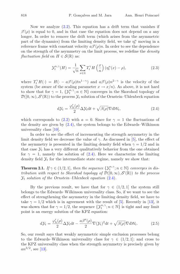
Now we analyze (2.2). This equation has a drift term that vanishes ifβ′(ρ) is equal to 0, and in that case the equation does not depend on a anylonger. In order to remove the drift term (which arises from the asymmetricpart of the dynamics) from the limiting density field, we take ηnt moving in areference frame with constant velocity aβ′(ρ)n. In order to see the dependenceon the strength of the asymmetry on the limit process, we redefine the densityfluctuation field on H ∈ S(R) as:
Yn,γt (H) =
1√n
∑
x∈Z
T γt H(xn
)(ηnt (x) − ρ), (2.3)
where T γt H(·) = H(· − aβ′(ρ)tn1−γ) and aβ′(ρ)n2−γ is the velocity of thesystem (be aware of the scaling parameter x → x/n). As above, it is not hardto show that for γ = 1, {Yn,γ
t ;n ∈ N} converges in the Skorohod topology ofD([0,∞),S ′(R)) to the process Yt solution of the Ornstein–Uhlenbeck equation
dYt =ϕ′h(ρ)2
ΔYtdt+√β(ρ)∇dWt, (2.4)
which corresponds to (2.2) with a = 0. Since for γ = 1 the fluctuations ofthe density are given by (2.4), the system belongs to the Edwards–Wilkinsonuniversality class [10].
In order to see the effect of incrementing the strength asymmetry in thelimit density field we decrease the value of γ. As discussed in [5], the effect ofthe asymmetry is presented in the limiting density field when γ = 1/2 and inthat case Yt has a very different qualitatively behavior from the one obtainedfor γ = 1, namely the solution of (2.4). Here we characterize the limitingdensity field Yt for the intermediate state regime, namely we show that:
Theorem 2.1. If γ ∈ (1/2, 1], then the sequence {Yn,γt ;n ∈ N} converges in dis-
tribution with respect to Skorohod topology of D([0,∞),S ′(R)) to the processYt solution of the Ornstein–Uhlenbeck equation (2.4).
By the previous result, we have that for γ ∈ (1/2, 1] the system stillbelongs to the Edwards–Wilkinson universality class. So, if we want to see theeffect of strengthening the asymmetry in the limiting density field, we have totake γ = 1/2 which is in agreement with the result of [5]. Recently in [13], itwas shown that for γ = 1/2, the sequence {Yn,γ
t ;n ∈ N} is tight and any limitpoint is an energy solution of the KPZ equation:
dYt =ϕ′h(ρ)2
ΔYtdt− aβ′′(ρ)2
∇(Yt)2dt+√β(ρ)∇dWt. (2.5)
So, our result says that weakly asymmetric simple exclusion processes belongto the Edwards–Wilkinson universality class for γ ∈ (1/2, 1]; and cross tothe KPZ universality class when the strength asymmetry is precisely given byan3/2, see [13].

Vol. 13 (2012) Crossover to the KPZ Equation 819
3. Beyond the Hydrodynamic Time Scale
In this section we give an outline of the proof of the equilibrium density andcurrent fluctuations in the intermediate state regime (with γ ∈ (1/2, 1]), i.e.between the Ornstein–Uhlenbeck process (2.4) and the KPZ equation (2.5).
3.1. Density Fluctuations
Here we prove Theorem 2.1. Recall the definition of the density fluctuationfield given in (2.3). In this setting, we remove the drift of the process, so thatwe suppose To have ηnt moving in a reference frame with constant velocitygiven by aβ′(ρ)n2−γ with γ ∈ (1/2, 1].
At t = 0, by computing the characteristic function of Yn,γ0 , this field con-
verges to a spatial white noise of variance χ(ρ). Now, we analyze the asymptoticbehavior of some martingales associated to Yn,γ
t , in order to identify the limitdensity field Yt as a weak solution of the stochastic partial differential equation(2.4). For that purpose, fix H ∈ S(R) and notice that by Dynkin’s formula,
Mn,γt (H) = Yn,γ
t (H) − Yn,γ0 (H) − In,γt (H) − An,γ
t (H)
is a martingale with respect to the natural filtration Ft = σ(ηs, s ≤ t), where
In,γt (H) =
t∫
0
12√n
∑
x∈Z
ΔnT γs H(xn
)(τxh(ηns ) − ϕh(ρ)) ds,
An,γt (H) =
t∫
0
n1−γ√n
∑
x∈Z
∇nT γs H(xn
)τxVf (ηns ) ds,
f(η) = ac(η)(η(1) − η(0))2/2,τxVf (η) = τxf(η) − aβ(ρ) − aβ′(ρ)(η(x) − ρ),
ΔnH(x/n) := n2(H((x+ 1)/n) +H((x− 1)/n) − 2H(x/n)) and∇nH(x) := n(H((x+ 1)/n) −H(x/n)).
Notice that Δn and ∇n are the discrete Laplacian and the discrete derivative,respectively. We point out that the mean of f with respect to νρ is given byaβ(ρ).
The quadratic variation of Mn,γt (H) equals to
〈Mn,γ(H)〉t =
t∫
0
12n
∑
x∈Z
(∇nT γs H
(xn
))2
τxf(ηns )(1 +
a
nγ
)ds.
We notice that if γ > 0, the term corresponding to a/nγ inside lastintegral, vanishes in L2(Pνρ
) as n → +∞. From now on, Pνρdenotes the dis-
tribution of the Markov process ηnt starting from the stationary state νρ andEνρ
denotes the expectation with respect to Pνρ. Last term arises from the
asymmetric part of the dynamics and for this reason, only for a big strengthof the asymmetry (namely for γ = 0; which corresponds to speeding up theasymmetric part of the dynamics by n2) it will give rise to additional stochasticfluctuations of the system. From simple computations, it follows that the limit

820 P. Goncalves and M. Jara Ann. Henri Poincare
as n → +∞ of the martingale Mn,γt (H) is given by ||√β(ρ)∇H||2Wt(H),
where Wt(H) is a Brownian motion and || · ||2 denotes the L2(R)-norm.Now, we need to analyze the limit of the integral terms. We start by
the less demanding, namely In,γt (H). Invoking the Boltzmann–Gibbs princi-ple introduced in [18], In,γt (H) can be written as
t∫
0
Yn,γs
(ϕ′h(ρ)2
ΔnH
)ds
plus an L2(Pνρ) negligible term.
Now we analyze An,γt (H). We notice that if we were considering the
case γ = 1 the Boltzmann-Gibbs principle as stated in [18], would be sayingthat An,γ
t (H) vanishes in L2(Pνρ) as n → +∞. Since γ < 1, the result in
[18] does not give us the information we need about the limit of this integralterm. Nevertheless, according to Corollary 7.4 of [12], it follows that in factfor γ ∈ (1/2, 1] the same result is true. Indeed the integral term An,γ
t (H) stillvanishes in L2(Pνρ
) as n → +∞ for γ ∈ (1/2, 1]. We remark that the men-tioned result in [12] was proved for the symmetric simple exclusion process butit is also true for our model. More explicitly, for our case that result says thefollowing:
Proposition 3.1 (Stronger Boltzmann–Gibbs Principle) [12]. Let ψ : Ω → R bea local function and let ϕψ(ρ) := Eνρ
[ψ(η)]. For γ ∈ (1/2, 1] and H ∈ S(R), itholds that
limn→∞ Eνρ
⎡
⎢⎣
⎛
⎜⎝t∫
0
n1−γ√n
∑
x∈Z
H(xn
)
×(τxψ(ηns ) − ϕψ(ρ) − ϕ′ψ(ρ)(ηns (x) − ρ))ds
)2
⎤
⎥⎦ = 0.
In [12], this result was proved for ψ(η) = (η(0)−ρ)(η(1)−ρ), but the proofholds for any local function, since the fundamental ingredients invoked alongthe proof, namely the spectral gap bound and the equivalence of ensembles,hold in general for local functions. As a consequence of last result, An,γ
t (H)still vanishes in L2(Pνρ
) as n → +∞ for γ ∈ (1/2, 1].Putting together the previous observations, for γ ∈ (1/2, 1], the limit
density field Yt(H) satisfies:
Yt(H) = Y0(H) +
t∫
0
Ys(ϕ′h(ρ)2
ΔH)
ds+ ||√β(ρ)∇H||2Wt(H),
Vol. 13 (2012) Crossover to the KPZ Equation 821
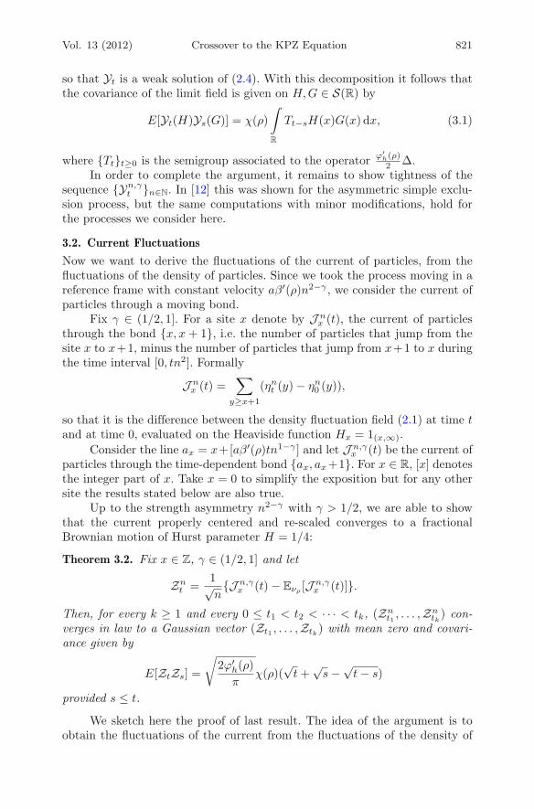
so that Yt is a weak solution of (2.4). With this decomposition it follows thatthe covariance of the limit field is given on H,G ∈ S(R) by
E[Yt(H)Ys(G)] = χ(ρ)∫
R
Tt−sH(x)G(x) dx, (3.1)
where {Tt}t≥0 is the semigroup associated to the operator ϕ′h(ρ)2 Δ.
In order to complete the argument, it remains to show tightness of thesequence {Yn,γ
t }n∈N. In [12] this was shown for the asymmetric simple exclu-sion process, but the same computations with minor modifications, hold forthe processes we consider here.
3.2. Current Fluctuations
Now we want to derive the fluctuations of the current of particles, from thefluctuations of the density of particles. Since we took the process moving in areference frame with constant velocity aβ′(ρ)n2−γ , we consider the current ofparticles through a moving bond.
Fix γ ∈ (1/2, 1]. For a site x denote by J nx (t), the current of particles
through the bond {x, x + 1}, i.e. the number of particles that jump from thesite x to x+1, minus the number of particles that jump from x+1 to x duringthe time interval [0, tn2]. Formally
J nx (t) =
∑
y≥x+1
(ηnt (y) − ηn0 (y)),
so that it is the difference between the density fluctuation field (2.1) at time tand at time 0, evaluated on the Heaviside function Hx = 1(x,∞).
Consider the line ax = x+[aβ′(ρ)tn1−γ ] and let J n,γx (t) be the current of
particles through the time-dependent bond {ax, ax+1}. For x ∈ R, [x] denotesthe integer part of x. Take x = 0 to simplify the exposition but for any othersite the results stated below are also true.
Up to the strength asymmetry n2−γ with γ > 1/2, we are able to showthat the current properly centered and re-scaled converges to a fractionalBrownian motion of Hurst parameter H = 1/4:
Theorem 3.2. Fix x ∈ Z, γ ∈ (1/2, 1] and let
Znt =
1√n
{J n,γx (t) − Eνρ
[J n,γx (t)]}.
Then, for every k ≥ 1 and every 0 ≤ t1 < t2 < · · · < tk, (Znt1 , . . . ,Zn
tk) con-
verges in law to a Gaussian vector (Zt1 , . . . ,Ztk) with mean zero and covari-ance given by
E[ZtZs] =
√2ϕ′
h(ρ)π
χ(ρ)(√t+
√s− √
t− s)
provided s ≤ t.
We sketch here the proof of last result. The idea of the argument is toobtain the fluctuations of the current from the fluctuations of the density of
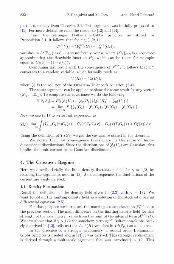
822 P. Goncalves and M. Jara Ann. Henri Poincare
particles, namely from Theorem 2.1. This argument was initially proposed in[19]. For more details we refer the reader to [12] and [14].
From the stronger Boltzmann–Gibbs principle as stated inProposition 3.1, it follows that for γ ∈ (1/2, 1]
J n,γ0 (t) − (Yn,γ
t (G�) − Yn,γ0 (G�)),
vanishes in L2(Pνρ) as � → +∞ uniformly over n, where {G�}�∈N is a sequence
approximating the Heaviside function H0, which can be taken for exampleequal to G�(x) = (1 − x/�)+.
Combining last result with the convergence of Yn,γt , it follows that Zn
t
converges to a random variable, which formally reads as
Yt(H0) − Y0(H0),
where Yt is the solution of the Ornstein-Uhlenbeck equation (2.4).The same argument can be applied to show the same result for any vector
(Zt1 , ..,Ztk). To compute the covariance we do the following:
E[ZtZs] = E[{Yt(H0) − Y0(H0)}{Ys(H0) − Y0(H0)}]= lim
�→+∞E[{Yt(G�) − Y0(G�)}{Ys(G�) − Y0(G�)}].
Now we use (3.1) to write last expression as
χ(ρ) liml→+∞
∫
R
(Tt−sG�(x)G�(x) −G�(x)TtG�(x) −G�(x)TsG�(x) +G2�(x)) dx.
Using the definition of Tt(G�) we get the covariance stated in the theorem.We notice that last convergence takes place in the sense of finite-
dimensional distributions. Since the distributions of Yt(H0) are Gaussian, thisimplies the limit current to be Gaussian distributed.
4. The Crossover Regime
Here we describe briefly the limit density fluctuation field for γ = 1/2, byrecalling the arguments used in [13]. As a consequence, the fluctuations of thecurrent are easily derived.
4.1. Density Fluctuations
Recall the definition of the density field given in (2.3) with γ = 1/2. Wewant to obtain the limiting density field as a solution of the stochastic partialdifferential equation (2.5).
For that purpose we introduce the martingales associated to Yn,γt as in
the previous section. The main difference on the limiting density field for thisstrength of the asymmetry, comes from the limit of the integral term An,γ
t (H).We saw above that if γ > 1/2 the somehow “stronger” Boltzmann-Gibbs prin-ciple derived in [12], tells us that An,γ
t (H) vanishes in L2(Pνρ) as n → +∞.
In the presence of a stronger asymmetry, a second order Boltzmann-Gibbs principle is needed and in [13] it was derived. This stronger replacementis derived through a multi-scale argument that was introduced in [12]. This

Vol. 13 (2012) Crossover to the KPZ Equation 823
multi-scale approach, allows to obtain the desired replacement as a sequenceof minor replacements in microscopic boxes that duplicate size at each step,until a point in which the sum of the errors committed at each step is neg-ligible and the last replacement holds at a box of small macroscopic size. Inthis macroscopic box, the non-trivial term can be identified as the square ofYn,γt . For details on this argument we refer the reader to [13]. The fundamen-
tal features of the model that are used in order to derive this second orderBoltzmann-Gibbs principle, are the sharp spectral gap bound for the dynam-ics restricted to finite boxes, plus a second order expansion on the equivalenceof ensembles. These results are quite general and this argument can be appliedfor more general models than of exclusion type.
With this procedure, in [13] was shown that for any H ∈ S(R), An,γt (H)
converges in L2(Pνρ) to
At(H) = limε→0
−β′′(ρ)2
t∫
0
∫
R
Ys(iε(x))2H ′(x) dxds. (4.1)
Here iε(x)(y) = ε−11(x<y≤x+ε).Applying the same arguments as above, in [13] it was shown that any
limit point of Yn,γt satisfies:
Yt(H) − Yγ0 (H) =
t∫
0
Ys(ϕ′h(ρ)2
ΔH)
ds+ At(H) + ||√β(ρ)∇H||2Wt(H)
with At(H) given as in (4.1). According to [13], the limit density field Yt is aweak solution of the KPZ equation (2.5).
4.2. Current Fluctuations
As mentioned above, having established the fluctuations of the density of par-ticles one can obtain the fluctuations of the current of particles J n,γ
0 (t). Fol-lowing the route described above, it follows that
1√n′ {J n′,γ
0 (t) − Eνρ[J n′,γ
0 (t)]}converges to
Yt(H0) − Y0(H0)
where Yt is the limit of the subsequence Yn′,γt and it is a weak solution of the
KPZ equation (2.5).So, the crossover regime for the current of particles occurs from Gaussian
to a distribution which is given in terms of the solution of the KPZ equation(2.5). As for the density of particles, the crossover of the current also occursat strength asymmetry an3/2.
In [1,21] the authors studied the weakly asymmetric simple exclusion pro-cess (which corresponds to taking c(·) ≡ 1 here) starting from different initialconditions. There, the crossover regime for the current of particles is studiedand the transition goes from Gaussian to Tracy–Widom distribution. For the

824 P. Goncalves and M. Jara Ann. Henri Poincare
strength asymmetry n3/2, [21] identify the limit distribution of the current asthe difference of two Fredholm determinants which, from the random matrixtheory, is known to converge to the Tracy–Widom distribution.
In [13], the stationary situation is studied and the limit of the currentis written in terms of the energy solution of the KPZ equation. The resultis true for a general class of weakly asymmetric exclusion processes. Here weshow that the transition from the Edwards–Wilkinson class to the KPZ classis universal within this class of processes and the strength asymmetry in orderto have the crossover is precisely an3/2. This is a step towards characterizingthe universality of the KPZ class.
Acknowledgements
P.G. would like to thank the warm hospitality of Universite Paris-Dauphine(France), where this work was initiated and to IMPA (Brazil) and CourantInstitute of Mathematical Sciences (USA), where this work was finished. P.G.thanks to “Fundacao para a Ciencia e Tecnologia” for the research projectPTDC/MAT/109844/2009: “Non-Equilibrium Statistical Physics” and for thefinancial support provided by the Research Center of Mathematics of the Uni-versity of Minho through the FCT Pluriannual Funding Program.
References
[1] Amir, G., Corwin, I., Quastel, J.: Probability distribution of the free energy ofthe continuum directed random polymer in 1 + 1 dimensions. Commun. PureAppl. Math. 64(4), 466–537 (2011)
[2] Bodineau, T., Derrida, B.: Distribution of current in non-equilibrium diffusivesystems and phase transitions. Phys. Rev. E. 72(6), 066110 (2005)
[3] Bertini L., De Sole A., Gabrielli D., Jona-Lasinio G. and Landim C.: Fluctu-ations in stationary nonequilibrium states of irreversible processes. Phys. Rev.Lett. 87(4), 040601 (2001)
[4] Bertini, L., De Sole, A., Gabrielli, D., Jona-Lasinio, G., Landim, C.: Macroscopicfluctuation theory for stationary non-equilibrium states. J. Stat. Phys. 107(3–4),635–675 (2002)
[5] Bertini, L., Giacomin, G.: Stochastic Burgers and KPZ equations from particlesystems. Commun. Math. Phys. 183(3), 571–607 (1997)
[6] Balazs, M., Quastel, J., Sepplinen, T.: Fluctuation exponent of the KPZ/sto-chastic Burgers equation. J. Am. Math. Soc. 24(3), 683–708 (2011)
[7] De Masi, A., Presutti, E., Scacciatelli, E.: The weakly asymmetric simple exclu-sion process. Ann. Inst. H. Poincare Probab. Stat. 25(1), 1–38 (1989)
[8] Gartner, J.: Convergence towards Burgers’ equation and propagation of chaosfor weakly asymmetric exclusion processes. Stoch. Process. Appl. 27(2), 233–260(1988)
[9] Dittrich, P., Gartner, J.: A central limit theorem for the weakly asymmetricsimple exclusion process. Math. Nachr. 151, 75–93 (1991)

Vol. 13 (2012) Crossover to the KPZ Equation 825
[10] Edwards, S., Wilkinson, D.: The surface statistics of a granular aggregate.Proceedings of The Royal Society of London, Series A. Math. Phys. Sci. 381(1780), 17–31 (1982)
[11] Ferrari, P., Spohn, H.: Scaling limit for the space-time covariance of the station-ary totally asymmetric simple exclusion process. Commun. Math. Phys. 265(1),1–44 (2006)
[12] Goncalves, P.: Central limit theorem for a tagged particle in asymmetric simpleexclusion. Stoch. Process. Appl. 118(3), 474–502 (2008)
[13] Goncalves, P., Jara, M.: Universality of KPZ equation. arXiv:1003.4478 (2010)
[14] Jara, M.D., Landim, C.: Nonequilibrium central limit theorem for a taggedparticle in symmetric simple exclusion. Ann. Inst. H. Poincare Probab.Stat. 42(5), 567–577 (2006)
[15] Johansson, K.: Shape fluctuations and random matrices. Commun. Math.Phys. 209(2), 437–476 (2000)
[16] Kardar, M., Parisi, G., Zhang, Y.C.: Dynamic scaling of growing interfaces. Phys.Rev. Lett. 56(9), 889–892 (1986)
[17] Prolhac S. and Mallick K.: Cumulants of the current in a weakly asymmetricexclusion process. J. Phys. A 42(17), 175001 (2009)
[18] Rost, H.: Hydrodynamik gekoppelter Diffusionen: Fluktuationen im Gleichge-witch Lecture notes in Mathematics, vol. 1031. pp. 97–107. Springer, Ber-lin (1983)
[19] Rost H. and Vares M. E.: Hydrodynamics of a one-dimensional nearest neigh-bor model. In: Particle systems, random media and large deviations (Brunswick,Maine). Contemp. Math., vol. 41, pp. 329–342. American Mathematical Society,Providence (1985)
[20] Sasamoto, T., Spohn, H.: One-dimensional Kardar–Parisi–Zhang equation: anexact solution and its universality. Phys. Rev. Lett. 104(23), (2010)
[21] Sasamoto, T., Spohn, H.: The crossover regime for the weakly asymmetric simpleexclusion process. J. Stat. Phys. 140(2), 209–231 (2010)
[22] Spohn, H.: Large Scale Dynamics of Interacting Particles. Springer, Berlin(1991)
[23] Tracy, C., Widom, H.: Asymptotics in ASEP with step initial condition. Com-mun. Math. Phys. 290(1), 129–154 (2009)
[24] Tracy, C., Widom, H.: Total current fluctuations in the asymmetric exclusionmodel. J. Math. Phys. 50(9), 095204 (2009)
Patrıcia GoncalvesCMATCentro de Matematica da Universidade do MinhoCampus de Gualtar4710-057 Braga, Portugale-mail: [email protected];

826 P. Goncalves and M. Jara Ann. Henri Poincare
Milton JaraIMPA, Instituto Nacional de Matematica Pura e AplicadaEstrada Dona Castorina 110Jardim Botanico22460-320 Rio de Janeiro, Brazile-mail: [email protected]
and
Ceremade, UMR CNRS 7534Universite Paris, DauphinePlace du Marechal De Lattre De Tassigny75775 Paris Cedex 16, France
Communicated by Bernard Nienhuis.
Received: June 20, 2011.
Accepted: August 29, 2011.
![Space-time paraproducts for paracontrolled calculus, 3d ... · on the 3-dimensional torus [11, 37] and the stochastic Navier-Stokes equation with additive noise [35, 36]. The KPZ](https://img.pdfslide.us/doc/110x75/5f9168339ea2be06a97fae75/space-time-paraproducts-for-paracontrolled-calculus-3d-on-the-3-dimensional.jpg)


![1+1 dimensional Kardar-Parisi-Zhang equation: more ... · short KPZ, is entitled “Dynamic scaling of growing interfaces” [1], see also the early re-views [2,3,4]. They study the](https://img.pdfslide.us/doc/110x75/5f421b80e3512c64065870e9/11-dimensional-kardar-parisi-zhang-equation-more-short-kpz-is-entitled-aoedynamic.jpg)


![KPZ LINE ENSEMBLE - math.berkeley.edualanmh/papers/KPZLineEnsemble.pdf · KPZ LINE ENSEMBLE 4 It has been understood since the work of [9, 10, 4, 31] that the following definition](https://img.pdfslide.us/doc/110x75/5fbe5bfb3c273e5ced393683/kpz-line-ensemble-math-alanmhpaperskpzlineensemblepdf-kpz-line-ensemble.jpg)


![Energy solutions of KPZ are uniqueperkowsk/... · tel [FQ15]. A remarkable consequence is that the energy solution to the KPZ equation is not equal to the Cole-Hopf solution, but](https://img.pdfslide.us/doc/110x75/5fb1f790b7cf0a2a2b044395/energy-solutions-of-kpz-are-unique-perkowsk-tel-fq15-a-remarkable-consequence.jpg)