CROSS-VALIDATED LOCAL LINEAR NONPARAMETRIC

Statistica Sinica 14(2004), 485-512

CROSS-VALIDATED LOCAL LINEAR

NONPARAMETRIC REGRESSION

Qi Li and Jeff Racine

Texas A&M University and Syracuse University

Abstract: Local linear kernel methods have been shown to dominate local constant

methods for the nonparametric estimation of regression functions. In this paper

we study the theoretical properties of cross-validated smoothing parameter selec-

tion for the local linear kernel estimator. We derive the rate of convergence of

the cross-validated smoothing parameters to their optimal benchmark values, and

we establish the asymptotic normality of the resulting nonparametric estimator.

We then generalize our result to the mixed categorical and continuous regressor

case which is frequently encountered in applied settings. Monte Carlo simulation

results are reported to examine the finite sample performance of the local-linear

based cross-validation smoothing parameter selector. We relate the theoretical and

simulation results to a corrected AIC method (termed AICc) proposed by Hur-

vich, Simonoff and Tsai (1998) and find that AICc has impressive finite-sample

properties.

Key words and phrases: Asymptotic normality, data-driven bandwidth selection,

discrete and continuous data, local polynomial regression.

1. Introduction

There exists a rich body of literature on the estimation of unknown regres-sion functions using kernel weighted local linear methods; see Fan (1992, 1993),Ruppert and Wand (1994), Fan and Gijbels (1995), among others. The locallinear estimator has many attractive properties including the fact that it is min-imax efficient and is one of the best known approaches for boundary correction.While practitioners often encounter a mix of discrete and continuous data typesin applied settings, existing local linear methods do not handle the presence ofdiscrete data in a satisfactory manner. In this paper we propose a new local lin-ear estimator which smooths both the discrete and continuous regressors usingthe method of kernels. Since it is widely appreciated that data-driven smoothingparameter selection is a necessity in applied nonparametric settings, we proposeusing least squares cross-validation (CV) for selecting smoothing parameters forboth types of regressors. In particular, we derive the rate of convergence of thecross-validated smoothing parameters to their optimal benchmark values, andwe establish the asymptotic normality of the resulting nonparametric estimator.

486 QI LI AND JEFF RACINE

The results contained herein are new even when considering the case for whichthere exist only continuous regressors.

The CV method is one of the most widely used bandwidth selectors forkernel smoothing, despite the fact that the relative error of the cross-validatedbandwidths may be higher than that for some alternative selection methods, forexample, the plug-in method. In the presence of discrete regressors, however, theCV method is particularly attractive because it has the ability to automaticallyremove irrelevant discrete regressors by smoothing them out; see Hall, Racine andLi (2004) for a more detailed discussion on this and related issues. In this paperwe explicitly address the case for which each regressor has a unique bandwidth(i.e., the vector-valued smoothing parameter case). This leads to a set of con-ditions that ensure that cross-validation will lead to optimal smoothing for thelocal linear kernel estimator, and illustrates how plug-in methods may face somepractical problems because it can be difficult to select good initial smoothingparameter values that are required by the plug-in method. We show via simula-tions that the cross-validated local linear estimator is capable of out-performingthe local constant estimator in the presence of mixed data types. We also findthat the corrected AIC method proposed by Hurvich, Simonoff and Tsai (1998)has impressive finite-sample properties. After the submission of this paper, awork by Xia and Li (2002) was brought to our attention in which they study theasymptotic behavior of cross-validated bandwidth selection for local polynomialfitting in a time series regression model with a univariate continuous regressor;our paper differs from Xia and Li’s in that (i) we consider multivariate regres-sion models and (ii) we allow for the presence of mixed discrete and continuousregressors.

2. Cross-Validation and the Local Linear Estimator: The ContinuousRegressor Case

Consider a nonparametric regression model

yj = g(xj) + uj , j = 1, . . . , n, (2.1)

where xj is a continuous random vector of dimension q. Define the derivative of

g(x): β(x)def= ∇g(x) ≡ ∂g(x)/∂x (∇g(·) is a q × 1 vector).

Define δ(x) = (g(x), β(x)′)′, so δ(x) is a (q + 1) × 1 vector-valued functionwhose first component is g(x) and whose remaining q components are the firstderivatives of g(x). Taking a Taylor series expansion of g(xj) at xi, we getg(xj) = g(xi)+ (xj −xi)′β(xi)+Rij , where Rij = g(xj)− g(xi)− (xj −xi)′β(xi).We write (2.1) as

yj = g(xi) + (xj − xi)′∇g(xi) + Rij + uj

= (1, (xj − xi)′)δ(xi) + Rij + uj . (2.2)

CROSS-VALIDATED LOCAL LINEAR NONPARAMETRIC REGRESSION 487

A leave-one-out local linear kernel estimator of δ(xi) is obtained by a kernelweighted regression of yj on (1, (xj − xi)′) given by

δ−i(xi) =

(g−i(xi)β−i(xi)

)

=

∑

j =i

Wh,ij

(1, (xj−xi)′

xj−xi, (xj−xi)(xj−xi)′

)−1∑

j =i

Wh,ij

(1

xj−xi

)yj, (2.3)

where Wh,ij =∏q

s=1 h−1s w((xjs − xis)/hs) is the product kernel function and

hs = hs(n) is the smoothing parameter associated with the sth component of x.Define a (q + 1) × 1 vector e1 whose first element is one with all remaining

elements being zero. The leave-one-out kernel estimator of g(xi) is given byg−i(xi) = e′1δ−i(xi), and we choose h1, . . . , hq to minimize the least-squares cross-validation function given by

CV (h1, . . . , hq) =n∑

i=1

[yi − g−i(xi)]2. (2.4)

We use h = (h1, . . . , hq) to denote the cross-validation choices of h1, . . . , hq

that minimize (2.4). Having computed h we then estimate δ(x) by

δ(x) =

(g(x)β(x)

)

=

[n∑

i=1

Wh,ix

(1, (xi − x)′

xi − x, (xi − x)(xi − x)′

)]−1 n∑i=1

Wh,ix

(1

xi − x

)yi,

where Wh,ix =∏q

s=1 h−1s w((xis−xs)/hs), and we estimate g(x) by g(x) = e′1δ(x).

The following assumptions are used to establish the convergence of h1, . . . , hq

to their optimal benchmark values and to establish the asymptotic normality ofg(x).

(A1) (i) (xi, yi) are i.i.d. as (X,Y ); S, the support of X, is a compactset; E(yi|xi) = g(xi) almost surely; ui = yi − g(xi) has finite 4th moments.(ii) infx∈S f(x) ≥ ε > 0 for some (small) ε > 0. (iii) g(x), f(x) and σ2(x) =E(u2

i |xi = x) are all fourth order differentiable in S. (iv) Letting gss(x) denotethe second order derivative of g with respect to xs, then

∫gss(x)2f(x)dx > 0 for

all s = 1, . . . , q.(A2) w(·) : R→R is a bounded symmetric density function with

∫w(v)v4dv

< ∞, and is m times differentiable. Letting w(s)(·) denote the sth order derivativeof w(·), ∫ |w(s)(v)vs|dv < ∞ for all s = 1, . . . ,m, where m > max2+4/q, 1+q/2is a positive integer.


(A3) (h1, . . . , hq) ∈ Hn = (h1, . . . , hq)|(h1, . . . , hq) ∈ [0, η]q , and nh1 · · · hq

≥ tn, where η = η(n) is a positive sequence that goes to zero slower than theinverse of any polynomial in n, and tn is a sequence that diverges to +∞.

(A1) (iv) requires that g is not linear in any of its components. The assump-tion that h1, . . . , hq lie in a shrinking set given in (A3) is not as restrictive as itappears, since otherwise the kernel estimator will have a non-vanishing bias termresulting in an inconsistent estimator when the model is nonlinear. We rule outthe case for which g(x) is linear in any of its components xs. The two conditionson Hn in (A3) are similar to those used in Hardle and Marron (1985), and theybasically require that hs → 0 for all s, and nh1 · · ·hq → ∞ as n → ∞.

In Appendix A we show that the leading term of the cross-validation functionis given by

CVL(h1, . . . , hq) =∫ [

κ2

2

q∑s=1

gss(x)h2s

]2

f(x)dx +B0

nh1 · · · hq, (2.5)

where gss(x) is the second order derivative of g with respect to xs, B0 = κq∫

σ2(x)dx, κ =

∫w(v)2dv and κ2 =

∫w(v)v2dv.

Define as via hs = asn−1/(q+4) for s = 1, . . . , q. Then we have CVL(h1, . . . , hq)

= n−4/(q+4)χ(a1, . . . , aq), where

χ(a1, . . . , aq) =∫ [

κ2

2

q∑s=1

gss(x)a2s

]2

f(x)dx +B0

a1 · · · aq. (2.6)

Let a01, . . . , a

0q denote values of a1, . . . , aq that minimize χ subject to being

non-negative. Note that if a0s = 0 for some s, then we must have a0

t = ∞ forsome t = s. Since we have assumed that g is not linear in any of its components,we rule out the case for which a0

t = ∞ and assume that, for s = 1, . . . , q,

each a0s is uniquely defined and is finite. (2.7)

It is easy to see that (2.7) requires that, for all s = 1, . . . , q, gss(x) does notvanish almost everywhere (our assumption (A3)), for otherwise a0

s = ∞.Below we provide a necessary and sufficient condition for (2.7). Let zs = a2

s

(s = 1, . . . , q), and let A denote a q × q positive semidefinite matrix having its(t, s)th element given by At,s = (κ2/2)

∫gtt(x)gss(x)f(x)dx. Then (2.6) can be

re-written asχz(z1, . . . , zq) = z′Az +

B0√z1 · · · zq

, (2.8)

where z = (z1, . . . , zq)′ is a q × 1 vector. Let z01 , . . . , z0

q denote the values ofz1, . . . , zq that minimize χz(z1, . . . , zq) subject to the requirement that each of


them be non-negative. Then it is easy to see that each z0s is uniquely defined and

is finite if and only if A is a positive definite matrix. A being positive definiteensures that each z0

s is finite, for otherwise z′Az = ∞ (hence χz = ∞). Giventhat each zs

0 is finite, we must have z0s > 0 because otherwise B0/(z0

1 · · · z0q )

1/2 =∞. Thus, each z0

s must be positive and finite, which in turn implies that eacha0

s = (z0s )1/2 is positive and finite. Thus, (2.7) holds true if and only if A is

positive definite.This condition imposes some restrictions on the second order derivative func-

tions gss (s = 1, . . . , q), and is more intuitive than (2.7). For example, if q = 1, itrequires that g11(x1) is not a ‘zero function’ (i.e., cannot be equal to zero a.e.).When q = 2, it assumes that gss(x) is not identically zero for s = 1, 2, andthat [

∫g11(x)2dF (x)][

∫g22(x)2dF (x)] > [

∫g11(x)g22(x)dF (x)]2 (F is the distri-

bution function of X). This last condition is equivalent to the requirement thatg11(x) − c g22(x) is not identically zero for any constant c.

While it is easy to obtain a closed form solution for as0 from (2.6) for q = 1, 2,

in the general multivariate q case there do not exist closed form solutions forthe a0

s’s (s = 1, . . . , q), even though they are well defined for any values of q.Therefore, a plug-in method based on (2.6) does not possess closed form solutions,and it seems difficult to obtain good initial values for the hs’s (s = 1, . . . , q) thatare required by the plug-in method.

We note here that it is important to explicitly allow for different values ofhs for the different components of xs (s = 1, . . . , q). If one were to use a scalarh1 = · · · = hq = h, as is often done to simplify the theoretical derivations (e.g.,Racine and Li (2003)), then one would not get the positive definiteness of A. Tosee this, note that if one were to use h1 = · · · = hq = h, and a1 = · · · = aq = a,then (2.6) becomes

χ(a) = a4∫ [

κ2

2

q∑s=1

gss(x)

]2

f(x)dx +B0

aq. (2.9)

Therefore, there exists a unique positive and finite a0 that minimizes χ(a) if∑qs=1 gss(x) is not a zero function. But this condition clearly does not give

applied researchers correct guidance as it would assert that hs converges to zeroeven if g(x) is linear in xs as long as g(x) is non-linear in some other componentsuch that

∑qs=1 gss(x) is not a zero function. Since in practice one never forces

all hs’s to be the same, (2.9) fails to reveal the correct conditions that ensure(2.7).

Let h01, . . . , h

0q denote the values of h1, . . . , hq that minimize (2.5). We have

h0s = a0

sn−1/(q+4). Also, given the fact that CVL is the leading term of CV , one

can show that hs = h0s + op(h0

s).


Theorem 2.1. Under (A1) through (A3) and (2.7), we have, for all s = 1, . . . , q,

(hs − h0s)/h

0s = Op(n−ε/(4+q)) with ε = minq/2, 2, where h0

s = a0sn

−1/(q+4).

For results on cross-validated local constant kernel regression, see Hardle,Hall and Marron (1988, 1992), and see Chen (1996) on using extra informationfor nonparametric smoothing in order to improve efficiency. With our result onecan establish the asymptotic normality of g(x).

Theorem 2.2. Under assumptions (A1) through (A3), and assuming that f(x) >

0, then√

nh1 · · · hq

[g(x) − g(x) − κ2

2

q∑s=1

gss(x)h2s

]→ N(0,Ωx) in distribution,

where Ωx = κqσ2(x)/f(x).

Under the assumption that g(·) is a smooth function with non-vanishingsecond-order derivatives, Theorems 2.1 and 2.2 show that hs converges to zero atthe rate Op(n−1/(4+q)) and that g(x) converges to g(x) at the rate Op(n−2/(4+q)).In practice, some regression functions g(·) may have a linear regression functionalform or be linear in some of their components (a partially linear specification).Our Theorem 2.1 does not cover such cases. However, it can be shown thatin the case for which g is linear in some of its components, say xs, then thecross-validation smoothing parameter hs will tend to take large numerical values,indicating that the model is partially linear. Note that our Theorem 2.1 doesnot cover a partially linear model since for a partially linear model, gss(x) = 0for some s ∈ 1, . . . , q, and Assumption (A1) (iv) is violated. In Section 3, weuse simulations to investigate the distribution of hs in this case. Our resultsexplain how the use of cross-validated local linear kernel methods in empiricalsettings may result in large smoothing parameters for some regressors and smallsmoothing parameters for others, a feature often exhibited in applied settings.

Up to now, we have restricted attention to the use of least squares cross-validation (CV) when selecting smoothing parameters. Hardle, Hall and Marron(1988) have shown that, for the local-constant estimator, the CV smoothing pa-rameter selectors are asymptotically equivalent to generalized CV (GCV) selec-tors, which include Akaike’s (1974) information criterion, Shibata’s (1981) modelselector, and Rice’s (1984) T selector, among others. It can easily be shown thatthe same conclusions hold true for the local linear method, that is, that thelocal-linear based CV smoothing parameter selector is asymptotically equivalentto the local-linear based GCV selector. This follows the exact same proof as inHardle, Hall and Marron (1988, p.95) as local-constant and local-linear estima-tors have the same rate of convergence (when both use a second order kernel).


Recently, Hurvich, Simonoff and Tsai (1998) suggested a corrected (improved)AIC criterion (termed AICc) as a smoothing parameter selector, and their simula-tions show that the AICc selector performs quite well compared with the plug-inmethod (when it is available) and with a number of generalized CV methods.While there is no theoretical result available for the AICc selector, we conjec-ture that the AICc selector is asymptotically equivalent to the (generalized) CVmethod, and simulation results are consistent with this conjecture. We find that,for small samples, AICc tends to perform better than the CV method, while forlarge samples there is no appreciable difference between the two methods.

Hardle, Hall and Marron (1988) also consider the intermediate benchmarkcase of selecting hs’s by minimizing the average square error given by ASE =n−1∑

i[g(xi)−g(xi)]2 for the univariate x case. They use h0 to denote the valuesof h that minimize ASE, and they further show that h − h0 = Op(n−1/10h0) =Op(n−3/10). This is the same rate as for h−h0 stated in our Theorem 2.1 for q = 1.We conjecture that Theorem 2.1 holds true when one replaces h0

s by h0s. This

is because one can show that CV = ASE + Op(η32 + η1(h1 · · ·hq)1/2) = ASE +

Op(ASE)Op(η2 + (h1 · · ·hq)1/2), where η2 =∑q

s=1 h2s and η1 = (nh1 · · ·hq)−1.

From this we expect that hs = h0s + Op(h0

s)Op((h0s)

min2,q/2), or equivalentlythat hs − h0

s = Op(n−1/(q+4)n−min[2,q/2]/(q+4)). However, a rigorous proof of thisresult lies beyond the scope of this paper.

3. Local Linear Cross Validation with Mixed Continuous and DiscreteRegressors

In this section we consider the case where a subset of regressors are categor-ical and the remaining are continuous. Although it is well known that one canuse a nonparametric frequency method to handle the discrete regressors (theo-retically), such an approach cannot be used in practice if the number of discretecells is large relative to the sample size, as is often the case with economic datasets containing mixed data types. Borrowing from Aitchison and Aitken’s (1976)approach, we elect to smooth the discrete regressors to circumvent this problem;see Hall (1981), Grund and Hall (1993), and the monographs by Scott (1992)and Simonoff (1996) for further discussion on the kernel smoothing of discretevariables.

Let xdi denote a r × 1 vector of regressors that assume discrete values and

let xci ∈ Rq denote the remaining continuous regressors. It should be mentioned

that Ahmad and Cerrito (1994) and Bierens (1983, 1987) also consider the caseof estimating a regression function with mixed categorical and continuous re-gressors, but they did not study the theoretical properties associated with us-ing data-driven methods (cross-validation) when selecting smoothing parameters.Furthermore, both works only consider the local constant kernel estimator.


For a discrete regressor, we use a variation on Aitchison and Aitken’s (1976)kernel function defined by

(xdis, x

djs) =

1, if xd

is = xdjs,

λs, otherwise.

The range of λs is [0,1]. Note that when λs = 0 the above kernel function becomesan indicator function, and when λs = 1, it is a constant function. That is, thexd

s regressor is removed (smoothed out) if λs = 1. Let 1(A) denote an indicatorfunction which assumes the value 1 if A holds true and 0 otherwise. Then theproduct kernel function for a vector of discrete regressors is given by

L(xdi , x

dj , λ) =

[r∏

s=1

λ1−1(xd

is=xdjs)

s

].

Now define the partial derivative of g(x) = g(xc, xd) with respect to xc:

β(x)def= ∇g(x) ≡ ∂g(xc, xd)/∂xc, and define δ(x) = (g(x), β(x)′)′. Also, we

use the short-hand notation Kh,ij = Wh,ijLλ,ij, where Wh,ij =∏q

s=1 h−1s w((xc

is −xc

js)/hs) and Lλ,ij =∏r

s=1 l(xdis, x

djs, λs). Then the leave-one-out kernel estimator

of δ(xi) ≡ δ(xci , x

di ) is given by

δ−i(xi) =

(g−i(xi)β−i(xi)

)

=

∑

j =i

Kh,ij

(1, (xc

j−xci )

′

xcj−xc

i , (xcj−xc

i)(xcj−xc

i)′

)−1∑

j =i

Kh,ij

(1

xcj−xc

i

)yj. (3.1)

Note that (3.1) treats the continuous regressor xc in a local linear fashion andthe discrete regressor xd in a local constant one. Again, g−i(xi) = e′1δ−i(xi)(e1 = (1, 0, . . . , 0)′), and we choose (h, λ) to minimize

CV (h1, . . . , hq, λ1, . . . , λr) =1n

n∑i=1

[yi − g−i(xi)]2 . (3.2)

We use (h1, . . . , hq, λ1, . . . , λr) to denote values of (h1, . . . , hq, λ1, . . . , λr) thatminimize (3.2). We then estimate g(x) by g(x) = e′1δ(x), where

δ(x) =

(g(x)β(x)

)

=

[∑i

Kh,ix

(1, (xc

i−xc)′

xci−xc, (xc

i−xc)(xci −xc)′

)]−1∑i

Kh,ix

(1

xci−xc

)yi,


with Kh,ix =∏q

s=1 h−1s w

((xc

is − xcs)/hs

)∏rs=1 l(xd

is, xds , λs).

In Appendix B we show that the leading term of the cross-validation functionis given by

CVL(h, λ) =∑xd

∫ κ2

2

q∑s=1

gss(x)h2s +

r∑s=1

Ds(x)λs

2

f(x)dxc +B0

nh1 · · ·hq,

(3.3)where gss(x) is the second order derivative of g(x) with respect to xc

s, B0 =κq ∑

xd

∫σ2(x) dxc, Ds(x) =

∑vd [1s(vd, xd) g(xc, vd) − g(x)] f(xc, vd) with

1s(xd, vd) = 1(xds = vd

s )∏

t=s 1(xdt = vd

t ), and 1s(xd, vd) = 1 if xd and vd dif-fers only in the sth component, and is 0 otherwise.

Define a1, . . . , aq, b1, . . . , br via hs = asn−1/(q+4) (s = 1, . . . , q) and λs =

bsn−2/(q+4) (s = 1, . . . , r). Then we have CVL(h, λ) = χ(a, b), where

χ(a, b) =∑xd

∫ κ2

2

q∑s=1

gss(x)a2s +

r∑s=1

Ds(x)bs

2

f(x)dxc +B0

h1 · · · hq.

Letting (a01, . . . , aq, b

01, . . . , b

0r) denote the values of (a1, . . . , aq, b1, . . . , br) that

minimize χ(a, b) subject to the restriction that they are non-negative, we fur-ther assume that

each of the a0s’s and b0

s’s is uniquely defined and is finite. (3.4)

Let h01, . . . , λ

0r denote the values of h1, . . . , λr that minimize (3.3). Then

obviously we have n1/(q+4)h0s ∼ a0

s for s = 1, . . . , q, and n2/(q+4)λ0s ∼ b0

s for s =1, . . . , r. In Appendix B we show that hs = h0

s + op(h0s) for s = 1, . . . , q, and that

λs = λ0s + op(λ0

s) for s = 1, . . . , r.

Theorem 3.1. Under (B1) and (B2) given in Appendix B, and (3.4), we have(hs − h0

s)/h0s = Op(n−ε1/(4+q)) for s = 1, . . . , q, and λs − λ0

s = Op(n−ε2) fors = 1, . . . , r, where ε1 = minq/2, 2, ε2 = min1/2, 4/(4 + q).

Combining Theorem 3.1’s rate of convergence result with a Taylor expansionargument, it is easy to establish the asymptotic normal distribution of g(x) asthe next theorem shows. The argument is sketched in Appendix B.

Theorem 3.2. Under the conditions of Theorem 3.1, we have

√nh1 · · · hq

(g(x) − g(x) −

2∑s=1

(κ2/2)gss(x)h2s −

r∑s=1

λsDs(x)

)→ N(0,Ωx)

in distribution,


where Ds(x) =∑

vd [1s(vd, xd)g(xc, vd) − g(x)]f(xc, vd), Ωx = κqσ2(x)/f(x).

From the discussion found in Section 2 we know that when g(x) is linearin xc

s, hs will not converge to zero, rather, hs will tend to take large values.Similarly, if g(x) turns out to be unrelated to xd

s (xds is an irrelevant regressor), it

can be shown that λs will not converge to zero, rather, it will tend to the upperbound value of 1. The theoretical results presented in this section do not coverthese cases. We rely on some simulation exercises to examine the finite samplebehavior of hs and λs when g(x) is linear in xc

s and/or is unrelated to xds .

The Ordered Categorical Regressor Case

Up to now we have only considered the case for which xd is unordered. If xds

is an ordered regressor, we use the following kernel function:

l(xdis, x

djs, λs) =

1, if xdis = xd

js,

λ|xd

is−xdjs|

s , if xdis = xd

js.

The range of λs is [0, 1]. Again when λs = 0, (lxdis, x

djs, λs = 0) becomes an

indicator function, and when λs = 1, l(xdis, x

djs, λs = 1) = 1 is a uniform weight

function.It is easy to show that the results of Theorems 3.1 and 3.2 remain valid

provided we redefine 1s(vd, xd) by 1s(vd, xd) = 1(|xds − vd

s | = 1)∏

t=s 1(xdt = vd

t )when xd

s is an ordered regressor.

4. Monte Carlo Results

In this section we examine the finite-sample behavior of cross-validated locallinear regression in the presence of mixed data types. In particular, we considerthree data generating processes (DGPs), one that is nonlinear in the continuousregressors, one that is linear, and one that lies in-between (i.e., is partially linear).These are given by

DGP1: yi = 1 + zi1 + zi2 + xi1xi2 + sin(2πxi1) + sin(2πxi2) + ui,

DGP2: yi = 1 + zi1 + zi2 + xi1 + xi2 + xi1xi2 + 2 sin(2xi2) + ui,

DGP3: yi = 1 + zi1 + zi2 + xi1 + xi2 + ui,

where X1 ∼ N(0, 1), X2 ∼ N(0, 1), Z1 ∈ 0, 1 with Pr[Z1 = 1] = 0.4,Z2 ∈ 0, 1 with Pr[Z2 = 1] = 0.6, and U ∼ N(0, σ2) with σ = 1.0. Wecompare the performance of six estimators: LIN: OLS assuming linearity and nointeraction; DGP: OLS based upon the correct DGP; LL(CV): Cross-validated


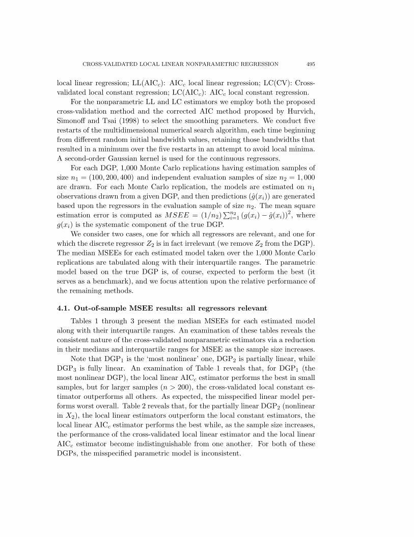
local linear regression; LL(AICc): AICc local linear regression; LC(CV): Cross-validated local constant regression; LC(AICc): AICc local constant regression.

For the nonparametric LL and LC estimators we employ both the proposedcross-validation method and the corrected AIC method proposed by Hurvich,Simonoff and Tsai (1998) to select the smoothing parameters. We conduct fiverestarts of the multidimensional numerical search algorithm, each time beginningfrom different random initial bandwidth values, retaining those bandwidths thatresulted in a minimum over the five restarts in an attempt to avoid local minima.A second-order Gaussian kernel is used for the continuous regressors.

For each DGP, 1,000 Monte Carlo replications having estimation samples ofsize n1 = (100, 200, 400) and independent evaluation samples of size n2 = 1, 000are drawn. For each Monte Carlo replication, the models are estimated on n1

observations drawn from a given DGP, and then predictions (g(xi)) are generatedbased upon the regressors in the evaluation sample of size n2. The mean squareestimation error is computed as MSEE = (1/n2)

∑n2i=1 (g(xi) − g(xi))

2, whereg(xi) is the systematic component of the true DGP.

We consider two cases, one for which all regressors are relevant, and one forwhich the discrete regressor Z2 is in fact irrelevant (we remove Z2 from the DGP).The median MSEEs for each estimated model taken over the 1,000 Monte Carloreplications are tabulated along with their interquartile ranges. The parametricmodel based on the true DGP is, of course, expected to perform the best (itserves as a benchmark), and we focus attention upon the relative performance ofthe remaining methods.

4.1. Out-of-sample MSEE results: all regressors relevant

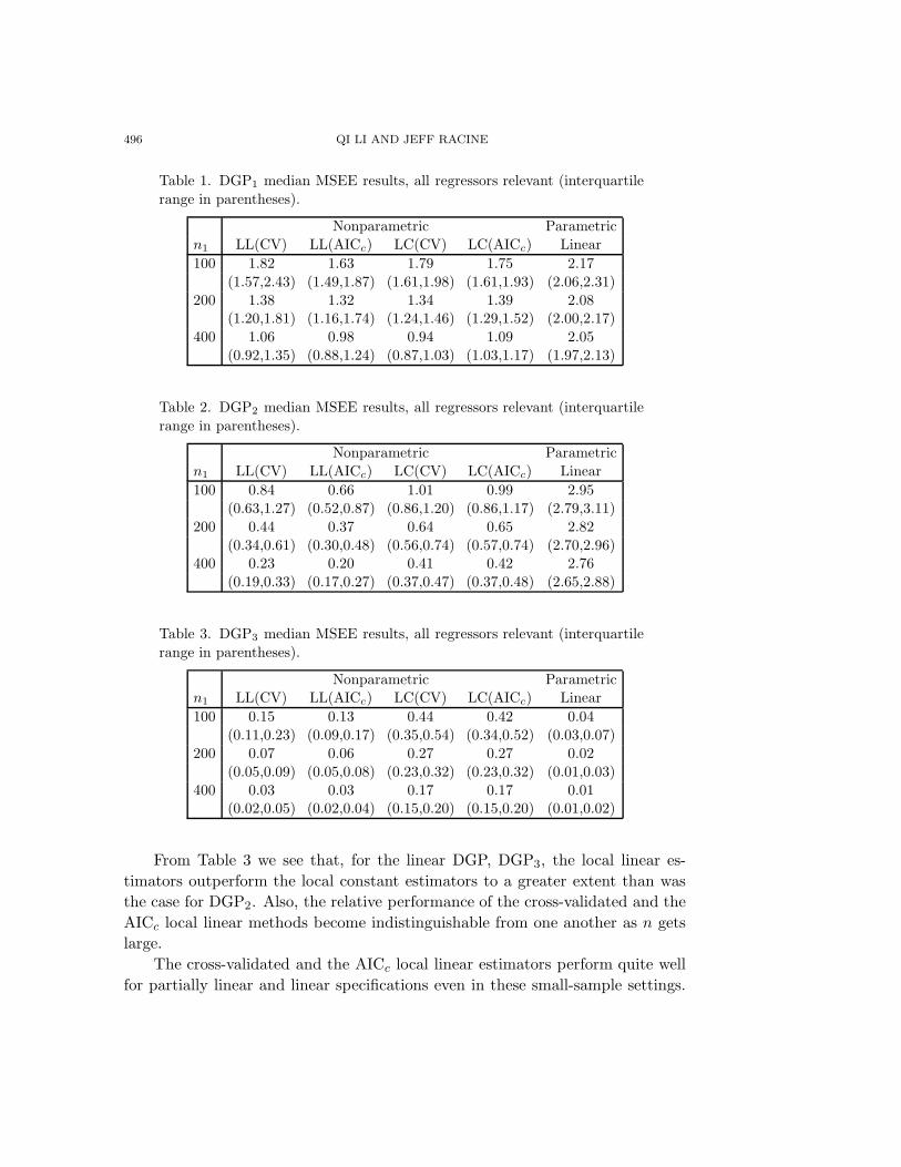
Tables 1 through 3 present the median MSEEs for each estimated modelalong with their interquartile ranges. An examination of these tables reveals theconsistent nature of the cross-validated nonparametric estimators via a reductionin their medians and interquartile ranges for MSEE as the sample size increases.

Note that DGP1 is the ‘most nonlinear’ one, DGP2 is partially linear, whileDGP3 is fully linear. An examination of Table 1 reveals that, for DGP1 (themost nonlinear DGP), the local linear AICc estimator performs the best in smallsamples, but for larger samples (n > 200), the cross-validated local constant es-timator outperforms all others. As expected, the misspecified linear model per-forms worst overall. Table 2 reveals that, for the partially linear DGP2 (nonlinearin X2), the local linear estimators outperform the local constant estimators, thelocal linear AICc estimator performs the best while, as the sample size increases,the performance of the cross-validated local linear estimator and the local linearAICc estimator become indistinguishable from one another. For both of theseDGPs, the misspecified parametric model is inconsistent.


Table 1. DGP1 median MSEE results, all regressors relevant (interquartilerange in parentheses).

Nonparametric Parametricn1 LL(CV) LL(AICc) LC(CV) LC(AICc) Linear100 1.82 1.63 1.79 1.75 2.17

(1.57,2.43) (1.49,1.87) (1.61,1.98) (1.61,1.93) (2.06,2.31)200 1.38 1.32 1.34 1.39 2.08

(1.20,1.81) (1.16,1.74) (1.24,1.46) (1.29,1.52) (2.00,2.17)400 1.06 0.98 0.94 1.09 2.05

(0.92,1.35) (0.88,1.24) (0.87,1.03) (1.03,1.17) (1.97,2.13)



(0.63,1.27) (0.52,0.87) (0.86,1.20) (0.86,1.17) (2.79,3.11)200 0.44 0.37 0.64 0.65 2.82

(0.34,0.61) (0.30,0.48) (0.56,0.74) (0.57,0.74) (2.70,2.96)400 0.23 0.20 0.41 0.42 2.76

(0.19,0.33) (0.17,0.27) (0.37,0.47) (0.37,0.48) (2.65,2.88)



(0.11,0.23) (0.09,0.17) (0.35,0.54) (0.34,0.52) (0.03,0.07)200 0.07 0.06 0.27 0.27 0.02

(0.05,0.09) (0.05,0.08) (0.23,0.32) (0.23,0.32) (0.01,0.03)400 0.03 0.03 0.17 0.17 0.01

(0.02,0.05) (0.02,0.04) (0.15,0.20) (0.15,0.20) (0.01,0.02)

From Table 3 we see that, for the linear DGP, DGP3, the local linear es-timators outperform the local constant estimators to a greater extent than wasthe case for DGP2. Also, the relative performance of the cross-validated and theAICc local linear methods become indistinguishable from one another as n getslarge.

The cross-validated and the AICc local linear estimators perform quite wellfor partially linear and linear specifications even in these small-sample settings.


Next we turn to the case when there exist irrelevant regressors.

4.2. Out-of-sample MSEE results: Z2 irrelevant

We now consider the case where one of the discrete regressors, Z2, is infact irrelevant. In this case, both the cross-validation and the AICc methodscan automatically remove such regressors by assigning them a large value of λ2,the associated bandwidth. We base this simulation upon the same DGPs givenabove. However, now Z2 is, in fact, irrelevant and is removed from the DGPwhen we generate Y . Furthermore, we do not assume that this information isknown a priori. Therefore, Z2 is still used for estimating the conditional meanof Y . MSEE results are presented in Tables 4 through 6.

Tables 4 through 6 illustrate that, in the presence of an irrelevant discreteregressor, the cross-validated local linear (constant) estimator and the AICc locallinear (constant) estimator display behavior similar to the case for which allregressors are relevant. The cross-validated local constant estimator outperformsthe cross-validated and AICc local linear estimators for the nonlinear DGP1 forn > 200, while Tables 5 and 6 reveal that, for the partially linear DGP2 (nonlinearin X2) and the linear DGP3, the local linear estimators outperform the localconstant estimators.

Table 4. DGP1 median MSEE results, Z2 irrelevant (interquartile range inparentheses).


(1.40,2.27) (1.33,1.84) (1.43,1.78) (1.42,1.73) (2.06,2.29)200 1.24 1.16 1.17 1.21 2.09

(1.06,1.71) (0.99,1.60) (1.07,1.28) (1.12,1.33) (2.00,2.19)400 0.96 0.88 0.77 0.90 2.04

(0.81,1.31) (0.78,1.14) (0.70,0.84) (0.80,1.00) (1.96,2.13)



(0.47,1.03) (0.37,0.72) (0.69,1.00) (0.67,0.95) (2.77,3.10)200 0.34 0.26 0.51 0.49 2.81

(0.24,0.51) (0.20,0.39) (0.44,0.61) (0.42,0.58) (2.68,2.95)400 0.17 0.14 0.32 0.32 2.77

(0.13,0.26) (0.11,0.20) (0.28,0.38) (0.27,0.37) (2.64,2.88)




(0.06,0.17) (0.05,0.11) (0.26,0.42) (0.24,0.37) (0.03,0.07)200 0.04 0.04 0.20 0.19 0.02

(0.03,0.07) (0.02,0.05) (0.17,0.25) (0.16,0.23) (0.01,0.03)400 0.02 0.02 0.13 0.12 0.01

(0.01,0.03) (0.01,0.03) (0.11,0.15) (0.10,0.14) (0.01,0.02)

Next we consider the behavior of the cross-validated bandwidths. We expectthat the local linear cross-validation method will tend to select a large band-width when the underlying DGP is in fact linear in a given continuous regressor,while the local constant estimator will display no such tendencies. For the cross-validated bandwidths for the irrelevant regressor Z2, we have postulated thatboth the local linear and local constant cross-validation methods will tend toselect a large bandwidth for an irrelevant discrete regressor, i.e., choose λ2 thattends toward its upper bound value of 1.

In an attempt to verify the above conjectures, we plot histograms of the cross-validated bandwidths for X1 (h1), X2 (h2), Z1 (λ1) and Z2 (λ2) for n1 = 200for DGP2. The results are presented in Figures 1 and 2, while Figures 3 and 4present comparable numbers for the AICc approach.

The histogram on the upper left of each figure summarizes the bandwidths forX1, the one on the upper right summarizes those for X2, the one on the lower leftsummarizes those for Z1, while that on the lower right summarizes those for Z2.The uppermost histograms in Figure 1 (the partially linear DGP2) reveal how thelocal linear cross-validation method chooses much larger smoothing parametersfor a continuous regressor that enters linearly (X1) than for one that entersnonlinearly (X2). In contrast, Figure 2 shows that the local constant cross-validation choices of h1 and h2 both assume (relatively) small values. Similarresults hold when bandwidth choice is conducted via the AICc approach.

While both the local linear and local constant cross-validation methods selectsmall values of λ1, Figures 1 and 2 show that their choices of λ2 tend to assumelarge values close to their upper bound value of 1, thereby effectively removingthe irrelevant regressor Z2 from the nonparametric estimate. This ‘automaticremoval of irrelevant discrete variables’ property is an appealing feature of thecross-validation method in applied settings. Similar results hold when bandwidthchoice is conducted via the AICc approach.


h1

0e+

00

3e-

07

6e-

07

Den

sity

0.0e+00 4.0e+06 8.0e+06 1.2e+07

h

01

2

2

34

56

0.1 0.2 0.3 0.4

Den

sity

λ1

0.0

0.0 0.2 0.4 0.6 0.8

1.0

1.0

2.0

3.0

Den

sity

λ

01

2

2

34

56

0.0 0.2 0.4 0.6 0.8 1.0

Den

sity

Figure 1. Histograms of LL(CV) smoothing parameters for DGP2, n = 200,Z2 irrelevant.

h

01

1

23

45

0.1 0.2 0.3 0.4 0.5

Den

sity

h

02

2

46

810

0.05 0.10 0.15 0.20 0.25 0.30

Den

sity

λ1

0.0

0.0 0.2 0.4 0.6 0.8

1.0

1.0

2.0

3.0

Den

sity

λ

01

2

2

34

56

0.0 0.2 0.4 0.6 0.8 1.0

Den

sity

Figure 2. Histograms of LC(CV) smoothing parameters for DGP2, n = 200,Z2 irrelevant.


h1

0e+

00

0e+00 1e+07 2e+07 3e+07 4e+07

4e-

08

8e-

08

Den

sity

h

0

2

510

15

0.20 0.25 0.30

Den

sity

λ

01

1

23

45

6

0.0 0.2 0.4 0.6 0.8 1.0

Den

sity

λ

0

2

510

15

0.0 0.2 0.4 0.6 0.8 1.0

Den

sity

Figure 3. Histograms of LL(AICc) smoothing parameters for DGP2, n =200, Z2 irrelevant.

h

0

1

24

68

0.35 0.40 0.45 0.50 0.55 0.60

Den

sity

h

0

2

510

15

0.18 0.20 0.22 0.24 0.26 0.28 0.30

Den

sity

λ1

0.0

0.0 0.2 0.4 0.6 0.8

1.0

1.0

2.0

3.0

Den

sity

λ

0

2

510

15

0.0 0.2 0.4 0.6 0.8 1.0

Den

sity

Figure 4. Histograms of LC(AICc) smoothing parameters for DGP2, n =200, Z2 irrelevant.


Here we only report simulation results for the two-continuous regressor case.Simulations not repeated here also show that, for a model with more than oneregressor entering the model linearly or being close to linear, the local linearcross-validation method provides even larger relative efficiency gains over thelocal constant method.

As noted in Section 2, Hardle, Hall and Marron (1988) demonstrated that,for the local constant estimator, CV smoothing parameter selectors are asymp-totically equivalent to GCV selectors. We have included results based on theHurvich, Simonoff and Tsai’s (1998) AICc bandwidth selection criterion in Tables1 through 6 which reveal that this approach indeed appears to be asymptoticallyequivalent to the CV method, and has excellent finite sample performance. Weleave theoretical investigations of the AICc method (such as verifying our con-jecture that AICc is asymptotically equivalent to the CV method) as a topic forfuture research.

5. Concluding Remarks

In this paper we present theoretical and simulation-based evidence in supportof using data-driven methods such as cross-validation and AICc when choosingsmoothing parameters for the local linear kernel estimator in the presence ofmixed discrete and continuous data types. We find that the AICc approachhas impressive finite-sample properties. We demonstrate that efficiency gainsrelative to the local constant estimator are not only theoretically possible butcan be readily attained in finite-sample settings. The results presented in thispaper also explain the observations of Li and Racine (2001) who found thatnonparametric estimators with smoothing parameters chosen via cross-validationcan yield superior predictions relative to commonly used parametric methods forU.S. patent application data, Spanish consumption data and U.S. and Swedishlabor force participation data.

Acknowledgement

We would like to thank an anonymous referee, an associate editor, and aco-editor for their insightful comments which led to a substantially revised andimproved version of the paper. An earlier version of this paper addressed onlyscalar smoothing parameter settings, while the current version deals with thepractically important vector-valued smoothing parameter case which arose outof a suggestion from the associate editor. The nice small sample performanceof the AICc method was suggested to us by a referee. Li’s Research is partiallysupported by the Private Enterprise Research Center, Texas A&M University.Racine would like to thank the Center for Policy Research at Syracuse Universityfor their ongoing support.


A. Proofs of Theorem 2.1 and 2.2

We will use the notation An ∼ Bn to denote that An has the same probabilityorder as Bn. To simplify the proof, we first re-write (2.3) in an equivalent form.Define D−2

h , a q × q diagonal matrix with its sth diagonal element given by h−2s ,

i.e., D−2h = diag(h−2

s ). Inserting the identity matrix Iq+1 = G−1n Gn into the

middle of (2.3), where Gn =(1, 00, D−2

h

), we get

δ−i(xi) =[∑

j =i

Wh,ijGn

(1

xj − xi

)(1, (xj − xi)′)

]−1∑j =i

Wh,ijGn

(1

xj − xi

)yj

=[∑

j =i

Wh,ij

(1

D−2h (xj − xi)

)(1, (xj − xi)′)

]−1

×∑j =i

Wh,ij

(1

D−2h (xj − xi)

)yj. (A.1)

The advantage of using (A.1) in the proof is that (1/n)∑

j =i Wh,ij( 1D−2

h (xj−xi)

)(1, (xj − xi)′) converges in probability to a non-singular matrix.

Hence, we can analyze the denominator and numerator of (A.1) separately andthus simplify the derivations.

Substituting the Taylor expansion (2.2) into (A.1), we have

δ−i(xi) = δ(xi) +

1

n

∑j =i

Wh,ij

(1, (xj − xi)′

D−2h (xj − xi), D−2

h (xj − xi)(xj − xi)′

)−1

×1

n

∑i

Wh,ij

(1

D−2h (xj − xi)

)[Rij + uj]

≡ δ(xi) + A−12i A1i,

A1i =1n

∑j =i

Wh,ij

(1

D−2h (xj − xi)

)[Rij + uj],

A2i =

(fi, B′

1i

D−2h B1i, D−2

h B2i

),

where fi = n−1 ∑j =i Wh,ij, B1i = n−1 ∑

j =i Wh,ij(xj − xi), and B2i =n−1∑

j =i Wh,ij(xj − xi)(xj − xi)′. It is easy to show B1i = Op(η2) and B2i =Op(η2) (η2 =

∑qs=1 h2

s). Thus D−2h B1i and D−2

h B2i are both Op(1) random vari-ables.


Recall that e1 is a (q + 1) column vector whose first element is one with allother elements being zero. Using the partitioned inverse, we have e′1A2i−1 =( f−1

i + C1i, −C2i ), where C1i = f−2i B′

1i[D−2h (B2i − B1iB

′1if

−1i )]−1B1i, and C2i

= f−1i B′

1i[D−2h (B2i − B1iB

′1if

−1i )]−1. Note that both C1i and C2i are Op(η2)

random variables. Then

g−i(xi) = e′1δ−i(xi) = g(xi) + e′1[A2i ]−1A1i = g(xi) + (f−1i + C1i,−C2i)A1i

= g(xi) +1n

∑j =i

Wh,ij[Rij + uj]/fi

+1n

∑j =i

Wh,ij[Rij + uj][C1i − C2iD−2h (xj − xi)]

≡ g(xi) +1n

∑j =i

Wh,ij[Rij + uj]/fi + Mn,

where Mn = n−1∑j =i Wh,ij[Rij +uj][C1i −C2iD

−2h (xj −xi)], which has an order

smaller than n−1∑j =i Wh,ij[Rij + uj]/fi (smaller by a factor of η2 =

∑qs=1 h2

s

since both C1i and C2i are Op(η2)).Define Di = n−1∑

j =i Wh,ij[Rij +uj ]/fi. Then we have g(xi) = g(xi)+Di +Mn ≡ g(xi) + Mn, where g(xi) = g(xi) + Di.

We use the short-hand notation gi = g(xi), gi = g(xi), gi = g(xi). DefineCV0(h) in the same manner as CV (h) but with gi being replaced by gi. Then

CV0(h)def=∑

i

(yi − gi)2 =∑

i

(gi + ui − gi)2 =∑

i

[ui −Di]2

=∑

i

D2i − 2

∑i

uiDi +∑

i

u2i ≡ CV1(h) + n−1

∑i

u2i , (A.2)

CV1(h) =∑

i

D2i − 2

∑i

uiDi

= n−3∑

i

∑j =i

∑l =i

[RijRil + ujul + 2ujRil]Wh,ijWh,il/f2i

−2n−2∑

i

∑j =i

ui[Rij + uj]Wh,ij/fi. (A.3)

Note that minimizing CV0(h) over h1, . . . , hq is equivalent to minimizing CV1(h)because n−1∑

i u2i is not related to h1, . . . , hq.

A technical difficulty in handling (A.3) arises from the presence of the randomdenominator fi, but

1fi

=1fi

+(fi − fi)

f2i

+(fi − fi)2

f2i fi

. (A.4)


Define CV2(h) by replacing the random denominator fi in CV1(h) by fi.

CV2(h) def=n−3

∑i

∑j =i

∑l =i

RijRilWh,ijWh,il/f2i

+n−3

∑i

∑j =i

∑l =i

ujulWh,ijWh,il/f2i − 2n−2

∑i

∑j =i

uiujWh,ij/fi

+2n−3

∑i

∑j =i

∑l =i

ujRilWh,ijWh,il/f2i − n−2

∑i

∑j =i

uiRijWh,ij/fi

≡ S1 + S2 + 2S3,where the definition of Sj (j = 1, 2, 3) should be apparent.

Define η1 = (nh1 · · ·hq)−1 and η2 =∑q

s=1 h2s. Lemmas A.1 to A.3 below show

that S1 =∫[(κ2/2)

∑qs=1 gss(x)h2

s ]2f(x)dx + O(η32 + η1(h1 · · ·hq)1/2 + n−1/2η2

2),S2 = B0(nh1 · · ·hq)−1 + O(η1(η2 + (h1 · · ·hq)1/2 + n−1/2) and S3 = O(n−1/2η2

2),where B0 = κq

∫σ2(x)dx. Therefore,

CV2(h) = S1 + S2 + 2S3 =∫ [κ2

2

q∑s=1

gss(x)h2s

]2f(x)dx +

B0

nh1 · · ·hq

+O(η32 + η1(η2 + (h1 · · ·hq)−1 + n−1/2)

).

Let CVL(h) =∫[(κ2/2)

∑qs=1 gss(x)h2

s ]2f(x)dx+B0(nh1 · · · hq)−1 denote theleading term of CV2(h).

Letting h01, . . . , h

0q denote the values of h1, . . . , hq that minimize CVL(h),

then obviously we have h0s = n−1/(q+4)a0

s = O(n−1/(q+4)) for s = 1, . . . , q,where a′0s are defined below (2.6). Recall that h1, . . . , hq are the values ofh1, . . . , hq that minimize CV (h). Based on the fact that CV (h) = CVL(h) +O(η3

2 + η1η2 + η1(h1 · · ·hq)1/2)+ terms not related to h1, . . . , hq, we know thaths = h0

s + op(h0s) = Op(n−1/(q+4)) for s = 1, . . . , q.

From CV1(h) = CVL(h) + O(η32 + η1η2 + η1(h1 · · · hq)1/2 + n−1/2η2

2) andhs ∼ n−1/(q+4), we obtain CV1(h) = CVL(h) + O(η1(h1 · · ·hq)1/2) if q ≤ 3, andCV1(h) = CVL(h) + O(η3

2) if q ≥ 4. Using these results one can show thaths = h0

s + Op(h0sn

−q/[2(q+4)]) if q ≤ 3, and hs = h0s + Op(h0

sn−2/(q+4)) if q ≥ 4.

This completes the proof of Theorem 2.1.

Proof of Theorem 2.2. Define g(x) in the same manner as g(x), but with thehs’s in g(x) being replaced by h0

s’s. Then it is well established that (nh01 · · · h0

q)1/2

(g(x)−∑qs=1(h

0s)2µs(x)) → N(0,Ωx) in distribution. Using the result of Theorem

2.1 and a standard Taylor expansion argument (e.g., Racine and Li (2004)), it iseasy to check that g(x) − g(x) = op(

∑qs=1(h

0s)2 + (nh0

1 · · ·h0q)−1/2). Then using

hs = h0s + Op(h0

sn−ε/(4+q)), one has Theorem 2.2.


Below we present some lemmas that are used in the proof of Theorem 2.1.We write An = Bn + (s.o.) to denote the fact that Bn is the leading order termof An, while (s.o.) denotes terms of smaller order than Bn.

Lemma A.1. S1 =∫[(κ2/2)

∑qs=1 gss(x)h2

s ]2f(x)dx + O(η3

2 + η1(h1 · · · hq)1/2 +n−1/2η2

2).

Proof. S1 = n−3∑∑∑i=j =l RijRilWh,ijWh,il/f

2i + n−3∑∑

j =i R2ijW

2h,ij/f

2i ≡

S1a + S1b. Here S1a = [n−3∑∑∑i=j =l H1a(xi, xj , xl)], where H1a(xi, xj , xl) is

a symmetrized version of RijRilWh,ijWh,il/f2i given by H1a(xi, xj , xl) = (1/3)

RijRilWh,ijWh,il/f2i + RjiRjlWh,ijWh,jl/f

2j + RljRliWh,ljWh,il/f

2l .

We first compute E[RijWh,ijf−1i |xi]. By the assumption that g(.) is a four-

time continuously differentiable function we have, uniformly in i,

E[RijWh,ijf−1i |xi] = E [ gj − gi − (xj − xi)′∇gi ]Wh,ijf

−1i |xi

= (κ2/2)q∑

s=1

gss(xi)h2s + O(η3

2), (A.5)

where κ2 =∫

w(v)v2dv, gss(xi) = [∂2g(x)/∂x2s ]|x=Xi . Using (A.5) we have

E[H1a(xi, xj , xl)] = EE[RijWh,ijf−1i |xi]2

= E[κ2

2

q∑s=1

gss(xi)h2s

]2+ O

(η32

)

=∫ [κ2

2

2∑s=1

q∑s=1

gss(x)h2s

]2f(x)dx + O

(η32

), (A.6)

E[H1a(xi, xj, xl)|xi] ∼ E[RijRilWh,ijWh,il/f2i |xi]

= E[RijWh,ij|xi]E[RilWh,il|xi]/f2i = E[RijWh,ij|xi]/fi2

=[κ2

2

q∑s=1

gss(xi)h2s

]2+ O

(η32

). (A.7)

By (A.5), (A.6), (A.7), and the U-statistic H-decomposition, we have

S1a = E[H1a(xi, xj , xl)] +3n

∑i

E[H1a(xi, xj , xl)|Xi]−E[H1a(xi, xj , xl)]+(s.o.)

= E[H1a(xi, xj , xl)] + n−1/2O(η22

)+ O

(η1(h1 · · ·hq)1/2

)

=[κ2

2

q∑s=1

gss(x)h2s

]2f(x)dx + O

(η32 + η1(h1 · · ·hq)1/2 + n−1/2η2

2

). (A.8)

Note that in applying the U-statistic H-decomposition, we write the last termas (s.o.) because the last term in the decomposition is a degenerate U-statistic,


(the U-statistic (2/n(n − 1))∑

i

∑j>i Hn(zi, zj) is said to be a degenerate U-

statistic if E[Hn(zi, zj)|zi] = 0), and it can be easily shown that it has an orderof O(η1/2

2 η1(h1 · · ·hq)1/2) = o(η1(h1 · · · hq)1/2), so we write it as (s.o.). Theη

1/22 factor comes from Rij, and O(η1(h1 · · ·hq)1/2) comes from the standard

degenerate U-statistic result.

Next, we consider S1b. Defining H1b(xi, xj) = R2ijW

2h,ij(1/f

2i +1/f2

j )/2, thenS1b = n−1[n−2∑

i

∑j =i H1b(xi, xj)], and it is easy to see that E[H1b(xi, xj)] =

E[R2ijW

2h,ij/f

2i ] = O

(η2(h1 · · ·hq)−1

).

Similarly, one can easily show that E[H1b(xi, xj)|xi] = O(η2(h1 · · ·hq)−1

).

Thus, by the H-decomposition,

S1b =1n

E[H1b(xi, xj)] + 2n−1

∑i

(E[H1b(xi, xj)|xi]−E[H1b(xi, xj)]) + (s.o.)

= O (η2η1) . (A.9)

The lemma follows from (A.8) and (A.9).

Lemma A.2. S2 = B0(nh1 · · ·hq)−1 + O(η1(η2 + n−1/2 + (h1 · · · hq)1/2)

),

where B0 = κq∫

σ2(x)dx, with η1 = (nh1 · · ·hq)−1 and η2 =∑q

s=1 h2s.

Proof. S2 = n−3∑i

∑j =i

∑l =i ujulWh,ijWh,il/f

2i − 2n−2∑

i

∑j =i uiujWh,ij/fi

= n−3 ∑i

∑j =i u2

j W 2h,ij / f2

i + n−3 ∑ ∑ ∑i=j =l uj ul Wh,ij Wh,il − 2n−2∑

i

∑j =i uiujWh,ij/fi ≡ S2a + S2b − 2S2c.

Define H2a(zi, zj) = (1/2) (u2i / f2

i + u2j / f2

j )W 2h,ij , then S2a = n−1 [n−2∑∑

i=j H2a(zi, zj)]. Then E[H2a(zi, zj)] = E[u2i W

2h,ij/f

2i ] = E[σ2(xi)W 2

h,ij/f2i ]

= (h1 · · ·hq)−1[B0 + O(η2)], where B0 = κq∫

σ2(x)dx (κ =∫

w(v)2dv).Next, we see that

E[H2a(zi, zj)|zi] = (1/2)(u2i /f

2i )E[W 2

h,ij |zi] + E[(σ2(xj)/f2j )W 2

h,ij|zi]= (1/2)u2

i f−2i E[W 2

h,ij|xi] + (1/2)E[σ2(xj)W 2h,ij/f

2j |xi]

= (1/2)(h1 · · ·hq)−1f−1i κq[u2

i + σ2(xi)] + O(η2)= B0i(h1 · · ·hq)−1 + Op(η2(h1 · · ·hq)−1),

where B0i = (κq/2)f−1i [u2

i +σ2(xi)]. It is easy to check that B0 = E[B0i]. Hence,by the H-decomposition we have

S2a = n−1E[H2a(zi, zj)]+2n−1

∑i

(E[H2a(zi, zj)|zi]−E[H2a(zi, zj)])+(s.o.)

= (nh1 · · ·hq)−1[B0 + O(η2)] + Op(n−1/2η1),

where the Op(n−1/2η1) term comes from the second term of the H-decomposition.


Next, S2b can be written as a third-order U-statistic. S2b = [n−3∑∑∑i=j =l

H2b(zi, zj , zl)], where H2b(zi, zj , zl) is a symmetrized version of ujulWh,ijWh,il/f2i

given by

H2b(zi, zj , zl) = (1/3)[ujulWh,ijWh,il/f2i + uiulWh,ijWh,jl/f

2j

+ujuiWh,ljWh,il/f2l ].

Note that E[H2b(zi, zj , zl)|zj ] = 0 because E(ul|zj) = 0. Hence, the leadingterm of S2b is a second-order degenerate U-statistic: E[H2b(zi, zj , zl)|zi, zj ] =(1/3)uiujE[Wh,ljWh,il/f

2l |xi, xj ].

Straightforward calculation shows that E[Wh,ljWh,il/f2l |xi, xj ] = W

(2)h,ij/fi +

O(η2), where W(2)h,ij =

∏qs=1 h−1

s w(2)((xis −xjs)/hs), and w(2)(v) def=∫

w(u)w(v +u)du is the two-fold convolution kernel derived from w(·). Hence,

S2b = 3n−2

∑∑j =i

E[H2b(zi, zj , zl)|zi, zj ] + (s.o)

=n−2

∑∑j =i

uiujE[Wh,ljWh,il/f2l |zi, zj ] + (s.o.)

=[n−2(h1 · · ·hq)

∑∑j =i

uiujW(2)h,ij/fi + (s.o.)

]

= (n(h1 · · · hq)1/2)−1Z2b,n + (s.o.),

where Z2b,n = (n(h1 · · ·hq)1/2)n−2∑∑j =i uiujW

(2)h,ij/fi is a zero mean Op(1)

random variable.Finally, S2c = n−2∑

i

∑j =i uiujWh,ij/fi = (n(h1 · · ·hq)1/2)−1Z2c,n, where

Z2c,n = (n(h1 · · · hq)1/2)[n−2∑i

∑j =i uiujWh,ij/fi] is a zero mean Op(1) random

variable. The lemma follows.

Lemma A.3. S3 = Op(η2n−1/2).

Proof. S3 = n−2 ∑i

∑j =i ui Rij Wh,ij / fi − n−3 ∑

i

∑j =i

∑l =i Rij ul Wh,ij

Wh,il/f2i = n−2 ∑

i

∑j =i ui Rij Wh,ij / fi − n−3 ∑

i

∑j =i Rij uj W 2

h,ij / f2i −

n−3∑∑∑i=j =l RijulWh,ijWh,il/f

2i ≡ S3a − S3b − S3c.

S3a = n−2∑i

∑j =i H3a(zi, zj), where H3a(zi, zj) = (1/2)[uiRij/fi+ujRji/fj]

Wh,ij.We first compute [H3a(zi, zj)|zi]. [H3a(zi, zj)|zi] = (1/2)(ui/fi)E[RijWh,ij|xi],

and E[RijWh,ij|xi] = (κ2/2)∑q

s=1 gss(xi)h2s + Op(η2

2). Thus, we have

[H3a(zi, zj)|zi] = (κ2/4)(ui/fi) q∑

s=1

gss(xi)h2s + Op(η

3/22 )

≡

q∑s=1

B3ih2s + (s.o.),

where B3i,s = (κ2/4)(ui/fi)gss(xi).


Using H-decomposition and noting that E[H3a(zi, zj)] = 0, we have S3a =2n−1∑

i E[H3a(zi, zj)|zi] + (s.o.) = 2n−1∑i

∑qs=1 B3i,sh

2s + (s.o.) ≡ Op(n−1/2η2),

because n−1/2∑i B3i,s is a zero mean Op(1) random variable.

Next, for S3b it is easy to see that S3b = (nh1 · · · hq)−1Op(S3a) = Op((nh1 · · ·hq)−1η2n

−1/2)) = op(n−1/2η2).Finally we consider S3c. It can be written as a third-order U-statistic

S3c = n−3∑∑∑i=j =l H3c(zi, zj , zl), where H3c(zi, zj , zl) is a symmetrized ver-

sion of ulRijWh,ijWh,il/f2i . Obviously E[H3c,(i)(zi, zj , zl)] = 0 and it can eas-

ily be verified that E[H3c,(i)(zi, zj , zl)|zi] = (1/3)ui∑q

s=1 D3i,s, where D3i,s =(κ2/2)gss(xi) + O(η2). Therefore, by H-decomposition we have

S3c =3n

∑i

E[H3c(zi, zj , zl)|zi] + (s.o.) = n−1/2[ q∑

s=1

n−1/2∑

i

uiD3i,sh2s

]+ (s.o.)

≡ Op(η2n−1/2),

because n−1/2∑i uiD3i,s is a Op(1) random variable. The lemma follows.

B. Proof of Theorems 3.1 and 3.2

We first list the assumptions that will be used to prove Theorems 3.1 and3.2.

Let Gαµ denote the class of functions introduced in Robinson (1988) for α > 0,

and µ a positive integer: m ∈ Gαµ , if m(xc) is µ times differentiable, and m(xc)

and its partial derivatives (up to order µ) are all bounded by functions that havefinite αth moment.(B1) (i) We restrict (h1, . . . , hq, λ1, . . . , λr) ∈ [0, η]q+r to lie in a shrinking set,and nh1 · · ·hq ≥ tn (tn → ∞ as n → ∞). (ii) The kernel function w(·) satisfies(A2). (iii) f(x) is bounded below by a positive constant on S × Sd, the supportof X = (Xc,Xd).(B2) (i) Xi, Yin

i=1 are independent and identically distributed as (X,Y ), ui =Yi−g(Xi) has finite fourth moment. (ii) Defining σ2(x) = E[u2

i |Xi = x], σ2(·, xd),g(·, xd) and f(·, xd) all belong to G4

2 for all xd ∈ Sd. (iii) Define, with the Ds(x)’sdefined in (3.3),

∫ κ2

2

q∑s=1

gss(x)a2s +

r∑s=1

Ds(x)bs

2f(x)dx +

B0

h1 · · ·hq

is uniquely minimized at (a01, . . . , a

0q , λ

01, . . . , λ

0r), and each a0

s and b0s is finite.

Proof of Theorem 3.1. We first prove some intermediate results. Let xi =(xc

i , xdi ), and define β(xi) = [∂g(xc, xd

i )/∂xc]|xc=xci. Now define Rij = g(xj) −


g(xi)−β(xi)′(xcj−xc

i), which is equivalent to g(xj) = g(xi)+β(xi)′(xcj−xc

i)+Rij.Therefore, we have

yj = g(xj)+uj = g(xi)+(xcj−xc

i )′β(xi)+Rij +uj = (1, (xc

j−xci)

′)δ(xi)+Rij +uj,(B.1)

where δ(xi) = (g(xi), β(xi)′)′.We observe that (B.1) has a form similar to (2.2) for the continuous-regressor-

only case. Therefore, by following the same arguments as in Appendix A, onecan introduce CV0(h, λ), CV2(h, λ) and CV2(h, λ) in a manner analogous to thecontinuous-regressor-only case presented in Appendix A. By also using (A.4) withfi = n−1∑

j =i Kh,ij, and noting that supx∈S |f(x) − f(x)| = o(1), one can showthat

CV (h, λ) = CV2(h, λ) + Op(η3 + η−1/21 )Op(CV2(h, λ)) +

1n

∑i

u2i , (B.4)

where η3 =∑q

s=1 h2s +

∑rs=1 λs, and

CV2(h, λ) = n−3∑

i

∑j =i

∑l =i

RijRilKh,ijKh,il/f2i

+n−3∑

i

∑j =i

∑l =i

ujulKh,ijKh,il/f2i − 2n−2

∑i

∑j =i

uiujKh,ij/fi

+2n−3∑

i

∑j =i

∑l =i

ujRilKh,ijKh,il/f2i −

∑i

∑j =i

uiRijKh,ij/fi

≡ S1 + S2 + 2S3, (B.5)

where the definition of Sj (j = 1, 2, 3) should be apparent.By lemmas B.1 through B.3 we know that

S1 =∑xd

∫ κ2

2

q∑s=1

gss(x)h2s +

r∑s=1

Ds(x)λs

2

+Op(η33 + η1(h1 · · ·hq)1/2 + n−1/2η2

3),S2 = B0(nh1 · · · hq)−1 + Op(η1(η3 + n−1/2 + (h1 · · ·hq)1/2)) + (s.o.),S3 = Op(n−1/2η3). (B.6)

Note that the above results are almost the same as the continuous-regressorcase except that η2 =

∑qs=1 h2

s is replaced by η3 =∑q

s=1 h2s +

∑rs=1 λs, i.e., the

bias term needs to be modified to include terms of order O(λs) (s = 1, . . . , r).The variance term remains unchanged.

Combining (B.4), (B.5) and (B.6), and also dropping n−1∑i u2

i , since it isindependent of (h, λ), we get

CV2 =∑xd

∫ κ2

2

q∑s=1

gss(x)h2s+

r∑s=1

Ds(x)λs

2f(x)dxc+

B0

nh1 · · ·hq+(s.o.). (B.7)


Define a1, . . . , aq, b1, . . . , br via hs = asn−1/(q+4) (s = 1, . . . , q) and hs =

bsn−2/(q+4) (s = 1, . . . , r). If CVL(h, λ) denotes the leading term of CV2 at

(B.7), then CVL(h, λ) = χ(a, b), where

χ(a, b) =∫ ∑

xd

κ2

2

q∑s=1

gss(x)a2s +

r∑s=1

Ds(x)bs

2dxc +

B0

h1 · · ·hq.

Let (a01, . . . , b

0r) denote the values of (a1, . . . , br) that minimize χ(a, b). By

(3.4) we know that each of the a0s’s and b0

s’s is uniquely defined and is finite.Letting (h0

1, . . . , λ0r) denote the values of (h1, . . . , λr) that minimize CVL, then

obviously n1/(q+q)h0s ∼ a0

s for s = 1, . . . , q, and n2/(q+4)λ0s ∼ b0

s for s = 1, . . . , q.By arguments similar to those found in the proof of Theorem 2.1 of Racine

and Li (2004), it can be shown that CV = CVL + Op((h1 · · ·hq)1/2)Op(CVL) ifq ≤ 3, and CV = CVL+Op(

∑qs=1 h2

s)Op(CVL) if q ≥ 4. Using h0s = O

(n−1/(q+4)

)we get hs = h0

s + Op(h0sn

−q/[2(q+4)]), λs = λ0s + Op(n−1/2), if q ≤ 3; hs =

h0s + Op(h0

sn−2/(q+4)), λs = λ0

s + Op(n−4/(q+4)), if q ≥ 4, where s = 1, . . . , q forhs, and s = 1, . . . , r for λs. This completes the proof of Theorem 3.1.

Proof of Theorem 3.2. Define g(x) in the same manner as g(x) but with h0s’s

and λ0s’s replacing hs’ and λs’s. Then it is easy to see that (nh0

1 · · ·h0q)1/2(g(x)−

g(x) − (κ2/2)∑q

s=1 gss(x)(h0s)2 −

∑rs=1 Ds(x)λ0

s) → N(0,Ω(x)) in distribution.Next, using the results of Theorem 3.1 and a Taylor expansion argument, it

is easy to show that (g(x)− g(x)) = op(n−2/(q+4)), also h2s = (h0

s)2+op(n−2/(q+4))and λs = λ0

s + op(n−2/(q+4)). Theorem 3.2 follows from these results.

Lemma B.1. S1 =∫ (κ2/2)

∑qs=1 gss(x)h2

s +∑r

s=1 Ds(x)λ2s2f(x)dx + Op(η3

3 +η1(h1 · · ·hq)1/2 + n−1/2η2

3), where the Djs(x)’s are some functions defined in theproof of Theorem 3.2.

Lemma B.2. S2 = B0(nh1 · · ·hq)−1 + Op(η1(η3 + n−1/2 + (h1 · · ·hq)1/2)), whereB0 = κq ∑

xd

∫σ2(x)dxc.

Lemma B.3. S3 = Op(n−1/2η3).

The proofs of Lemmas B.1 through B.3 proceed along the lines of the proofsof Lemmas A.1 through A.3. Below we provide outlines of proofs for LemmasB.1 and B.2.

Proof of Lemma B.1. We have S1 = n−3∑∑∑i=j =l RijRilKh,ijKh,il/f

2i +

n−3∑∑j =i R

2ijK

2h,ij/f

2i ≡ S1a+S1b. The term S1a can be written as a third order

U-statistic whose leading term is E[RijRilKh,ijKh,il/f2i ]=EE[RijKh,ij/fi|xi]2.

Now

E[RijKh,ijf−1i |xi] = E [ gj − gi − (xc

j − xci )

′∇gi ]Kh,ijf−1i |xi


=κ2

2

q∑s=1

gi,ssh2s +

q∑s=1

λs

∑vd

[1s(xdi , v

d)g(xci , v

d) − g(xi)] + O(η23

),

where gi,ss = [∂2/∂(xcs)2g(x)]|x=Xi is the second partial derivative of g with

respect to xcs evaluated at xi. Therefore,

EE[RijKh,ij/fi|xi]2

= Eκ2

2

q∑s=1

gss(xi)h2s +

q∑s=1

λs

∑vd

[1s(xdi , v

d)g(xci , v

d) − g(xi)]2

+ O(η33

)

≡∑xd

∫ κ2

2

q∑s=1

gss(x)h2s +

∑s=1

λsDs(x)2

f(x)dxc + O(η33

),

where Ds(x) =∑

vd [1s(xd, vd)g(xc, vd) − g(x)]f(xc, vd).Similar to the arguments used in the proof of Lemma A.1, one can show that

S1 = EE[RijKh,ij/fi|xi]2+Op(η33 +η1(h1 · · ·hq)1/2 +n−1/2η2

3). This completesthe proof.

Proof of Lemma B.2. S2 =n−3∑i

∑j =i

∑l =i ujulKh,ijKh,il/f

2i −2n−2∑

i

∑j =i

uiujKh,ij/fi = n−3 ∑i

∑j =i u

2jK

2h,ij/f

2i + n−3∑∑∑

i=j =l ujulKh,ijKh,il − 2n−2∑i

∑j =i uiujKh,ij/fi ≡ S2a + S2b − 2S2c.

Along the lines of the proof of Lemma A.2, it can be shown that S2 =E(S2a)+ O(E(S2a)

(η3 + n−1/2 + (h1 · · ·hq)1/2

). The leading term of S2, E[S2a]

is

E[S2a] = n−1E[u2i K

2h,ij/f

2i ] = n−1E[σ2(xi)K2

h,ij/f2i ]

= (nh1 · · ·hq)−1[B0 + O(η3)],

where B0 = κqE[σ2(xi)/f(xi)], κ =∫

w(v)2dv. Thus, we have

S2 = E[S2a] + O(E(S2a)(η3 + n−1/2 + (h1 · · ·hq)1/2)

)=

B0

nh1 · · ·hq+ O

(η1(η3 + n−1/2 + (h1 · · ·hq)1/2)

).

This completes the proof of Lemma B.2.

References

Ahmad, I. A. and Cerrito, P. B. (1994). Nonparametric estimation of joint discrete-continuous

probability densities with applications, J. Statist. Plann. Inference 41, 349-364.

Aitchison, J. and Aitken, C. G. G. (1976). Multivariate binary discrimination by the kernel

method, Biometrika 63, 413-420.

Akaike, H. (1974). A new look at the statistical model identification, IEEE Trans. Automat.

Control 9, 716-723.


Bierens, H. (1983). Uniform consistency of kernel estimators of a regression function under

generalized conditions. J. Amer. Statist. Assoc. 78, 699-707.

Bierens, H. (1987). Kernel estimation of regression functions. In Advances in Econometrics

(Edited by T. F. Bewley). Cambridge University Press, Cambridge.

Chen, R. (1996). Incorporating extra information in nonparametric smoothing. J. Multivariate

Anal. 58, 133-150.

Fan, J. (1992). Design-adaptive nonparametric regression. J. Amer. Statist. Assoc. 87,

998-1004.

Fan, J. (1993). Local linear smoothers and their minimax efficiency. Ann. Statist. 21, 196-216.

Fan, J. and Gijbels, I. (1995). Local Polynomial Modeling and its Applications. Chapman and

Hall.

Grund, B. and Hall, P. (1993). On the performance of kernel estimators for high-dimensional

sparse binary data. J. Multivariate Anal. 44, 321-344.

Hall, P. (1981). On nonparametric multivariate binary discrimination. Biometrika 68, 287-294.

Hall, P., Racine, J. and Li, Q. (2004). Cross-validation and the estimation of conditional

probability densities. J. Amer. Statist. Assoc. To accept.

Hardle, W., Hall, P. and Marron, J. S. (1988). How far are automatically chosen regression

smoothing parameters from their optimum? J. Amer. Statist. Assoc. 83, 86-99.

Hardle, W., Hall, P. and Marron, J. S. (1992). Regression smoothing parameters that are not

far from their optimum. J. Amer. Statist. Assoc. 87, 227-233.

Hardle, W. and Marron, J. S. (1985). Optimal bandwidth selection in nonparametric regression

function estimation. Ann. Statist. 13, 1465-1481.

Hurvich, C. M. and Simonoff, J. S. and Tsai, C. L. (1998). Smoothing parameter selection in

nonparametric regression using an improved Akaike information criterion. J. Roy. Statist.

Soc. B 60, 271-293.

Li, Q. and Racine, J. (2001). Empirical applications of smoothing categorical variables. Un-

published manuscript.

Racine, J. and Li, Q. (2004). Nonparametric estimation of regression functions with both

categorical and continuous Data. J. Econometrics 119, 99-130.

Rice, J. (1984). Bandwidth choice for nonparametric regression. Ann. Statist. 12, 1215-1230.

Robinson, P. (1988). Root-N consistent semiparametric regression. Econometrica, 56, 931-954.

Ruppert, D. and Wand, M. P. (1994). Multivariate weighted least squares regression. Ann.

Statist. 22, 1346-1370.

Scott, D. (1992). Multivariate Density Estimation: Theory, Practice, and Visualization. Wiley,

New York.

Simonoff, J. S. (1996). Smoothing Methods in Statistics. Springer, New York.

Shibata, R. (1981). An optimal selection of regression variables. Biometrika 68, 45-54.

Xia, Y. C. and Li, W. K. (2002). Asymptotic behavior of bandwidth selected by the cross-

validation method for local polynomial fitting. J. Multivariate Anal. 83, 265-287.

Department of Economics, Texas A&M University, College Station, TX 77843-4228, U.S.A.

E-mail: [email protected]

Department of Economics and Center for Policy Research, Syracuse University, 426 Eggers Hall.

Syracuse, NY 13244-1020, U.S.A.

E-mail: [email protected]

(Received September 2002; accepted July 2003)

Documents

CROSS-VALIDATED LOCAL LINEAR NONPARAMETRIC