Embed Size (px)
Citation preview
The Consumption, Income, and Wealth of the Poorest:Cross-Sectional Facts of Rural and Urban Sub-Saharan Africa
for Macroeconomists
Leandro De Magalhães (University of Bristol)Raül Santaeulàlia-Llopis (Washington University in St. Louis)
ECAMA 2015
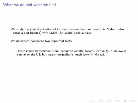
What we do and what we find
We study the joint distribution of income, consumption, and wealth in Malawi (alsoTanzania and Uganda) with LSMS-ISA World Bank surveys.
We document document two important facts:
1. There is low transmission from income to wealth. Income inequality in Malawi issimilar to the US, but wealth inequality is much lower in Malawi.
2. There is low transmission from income to consumption. Consumption inequalityis lower in Malawi than the US.
Our evidence points towards saving constraints and risk sharing.
The Micro Data: Integrated Surveys on Agriculture (ISA)
I For the case of Malawi, the country is divided in 27 district with 12,271households interviewed in 2010.
I The sample is rolled over 12 months from March 2010 to March 2011.
I The level of detail in consumption, income and wealth that you will see allows usto practically recover entire household-level budget constraints (This cannot bedone even for the US with a single data source).
Measuring Household Consumption
I The main consumption items for rural households are are food (65%), clothing(3%), utilities (16%), other nondurables (14%).
In urban areas food accounts forless (51%) and other non-durables for 19%.
I Food items are reported in different units (e.g. heaps, pail, basket, piece, bunchand others). They are converted using ’price conversion’.
I To estimate the value of own consumption and gifts, we use the medianconsumption price of the same item/unit in that season-region.
I Deseasonalization: Non-durable consumption is deseasonalized using IHS2(2004-5) and IHS3 (2010-11) monthly dummies.
Measuring Household Consumption
I The main consumption items for rural households are are food (65%), clothing(3%), utilities (16%), other nondurables (14%). In urban areas food accounts forless (51%) and other non-durables for 19%.
I Food items are reported in different units (e.g. heaps, pail, basket, piece, bunchand others). They are converted using ’price conversion’.
I To estimate the value of own consumption and gifts, we use the medianconsumption price of the same item/unit in that season-region.
I Deseasonalization: Non-durable consumption is deseasonalized using IHS2(2004-5) and IHS3 (2010-11) monthly dummies.
Measuring Household Income
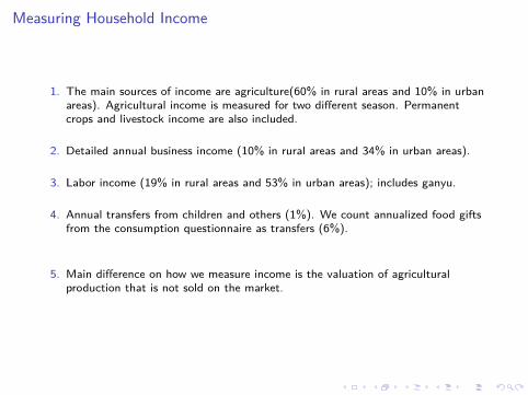
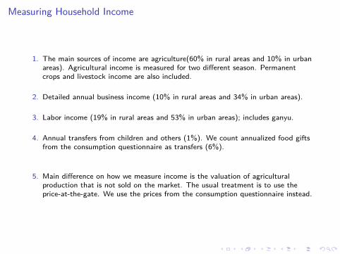
1. The main sources of income are agriculture(60% in rural areas and 10% in urbanareas). Agricultural income is measured for two different season. Permanentcrops and livestock income are also included.
2. Detailed annual business income (10% in rural areas and 34% in urban areas).
3. Labor income (19% in rural areas and 53% in urban areas); includes ganyu.
4. Annual transfers from children and others (1%). We count annualized food giftsfrom the consumption questionnaire as transfers (6%).
5. Main difference on how we measure income is the valuation of agriculturalproduction that is not sold on the market. The usual treatment is to use theprice-at-the-gate. We use the prices from the consumption questionnaire instead.
Measuring Household Income
1. The main sources of income are agriculture(60% in rural areas and 10% in urbanareas). Agricultural income is measured for two different season. Permanentcrops and livestock income are also included.
2. Detailed annual business income (10% in rural areas and 34% in urban areas).
3. Labor income (19% in rural areas and 53% in urban areas); includes ganyu.
4. Annual transfers from children and others (1%). We count annualized food giftsfrom the consumption questionnaire as transfers (6%).
5. Main difference on how we measure income is the valuation of agriculturalproduction that is not sold on the market.
The usual treatment is to use theprice-at-the-gate. We use the prices from the consumption questionnaire instead.
Measuring Household Income
1. The main sources of income are agriculture(60% in rural areas and 10% in urbanareas). Agricultural income is measured for two different season. Permanentcrops and livestock income are also included.
2. Detailed annual business income (10% in rural areas and 34% in urban areas).
3. Labor income (19% in rural areas and 53% in urban areas); includes ganyu.
4. Annual transfers from children and others (1%). We count annualized food giftsfrom the consumption questionnaire as transfers (6%).
5. Main difference on how we measure income is the valuation of agriculturalproduction that is not sold on the market. The usual treatment is to use theprice-at-the-gate. We use the prices from the consumption questionnaire instead.
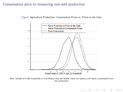
Consumption price to measuring non-sold production
Figure: Agricultural Production: Consumption Prices vs. Prices at the Gate
Note: Sample of 4,385 households in rural Malawi that sell neither maize nor tobacco and report consumption fromown production.
Measuring Household Wealth
I Land and housing is the main component wealth (more than 70% in both ruraland urban areas). These are self-reported value: “If you were to sell this [PLOT]today, how much could you sell it for?”
I But 80% of household also report there is no market for land in their area andland is seldom allocated through the market.
I This suggests that an important mechanism to accumulate wealth is not available.
I The other large components of wealth in rural areas besides land (46%) andhousing (27%), are livestock (11%) and agricultural equipment (3%). In urbanareas it is durables(27%), bicycle, TV, fridge etc..
Indications of a saving constraint
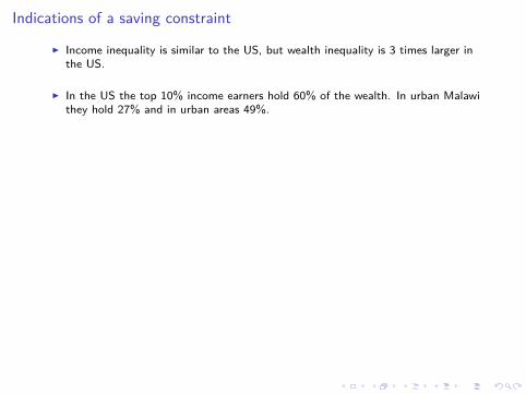
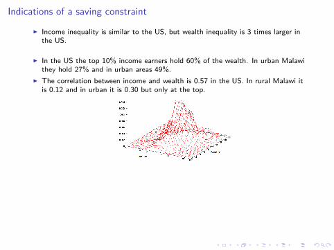
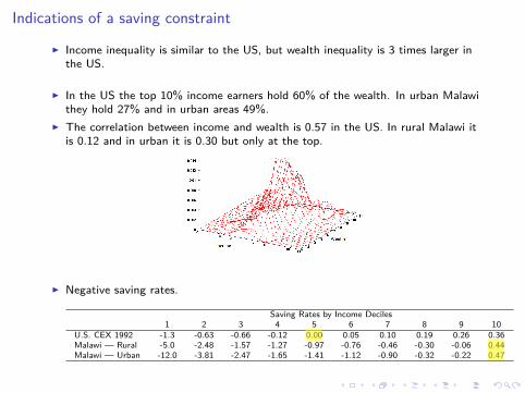
I Income inequality is similar to the US, but wealth inequality is 3 times larger inthe US.
I In the US the top 10% income earners hold 60% of the wealth. In urban Malawithey hold 27% and in urban areas 49%.
I The correlation between income and wealth is 0.57 in the US. In rural Malawi itis 0.12 and in urban it is 0.30 but only at the top.
I Negative saving rates.
Saving Rates by Income Deciles1 2 3 4 5 6 7 8 9 10
U.S. CEX 1992 -1.3 -0.63 -0.66 -0.12 0.00 0.05 0.10 0.19 0.26 0.36Malawi — Rural -5.0 -2.48 -1.57 -1.27 -0.97 -0.76 -0.46 -0.30 -0.06 0.44Malawi — Urban -12.0 -3.81 -2.47 -1.65 -1.41 -1.12 -0.90 -0.32 -0.22 0.47
Indications of a saving constraint
I Income inequality is similar to the US, but wealth inequality is 3 times larger inthe US.
I In the US the top 10% income earners hold 60% of the wealth. In urban Malawithey hold 27% and in urban areas 49%.
I The correlation between income and wealth is 0.57 in the US. In rural Malawi itis 0.12 and in urban it is 0.30 but only at the top.
I Negative saving rates.
Saving Rates by Income Deciles1 2 3 4 5 6 7 8 9 10
U.S. CEX 1992 -1.3 -0.63 -0.66 -0.12 0.00 0.05 0.10 0.19 0.26 0.36Malawi — Rural -5.0 -2.48 -1.57 -1.27 -0.97 -0.76 -0.46 -0.30 -0.06 0.44Malawi — Urban -12.0 -3.81 -2.47 -1.65 -1.41 -1.12 -0.90 -0.32 -0.22 0.47
Indication of risk sharing
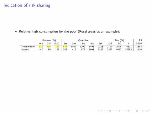
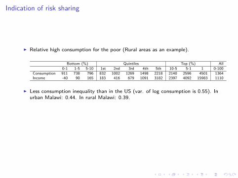
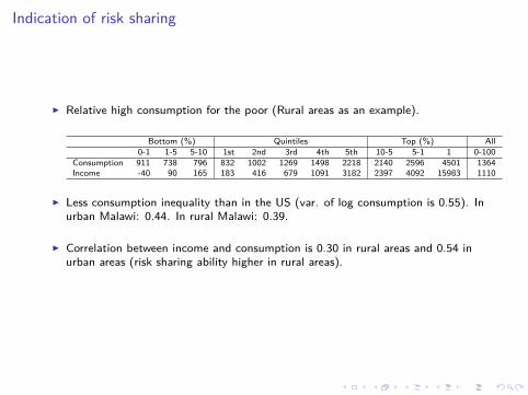
I Relative high consumption for the poor (Rural areas as an example).
Bottom (%) Quintiles Top (%) All0-1 1-5 5-10 1st 2nd 3rd 4th 5th 10-5 5-1 1 0-100
Consumption 911 738 796 832 1002 1269 1498 2218 2140 2596 4501 1364Income -40 90 165 183 416 679 1091 3182 2397 4092 15983 1110
I Less consumption inequality than in the US (var. of log consumption is 0.55). Inurban Malawi: 0.44. In rural Malawi: 0.39.
I Correlation between income and consumption is 0.30 in rural areas and 0.54 inurban areas (risk sharing ability higher in rural areas).
Indication of risk sharing
I Relative high consumption for the poor (Rural areas as an example).
Bottom (%) Quintiles Top (%) All0-1 1-5 5-10 1st 2nd 3rd 4th 5th 10-5 5-1 1 0-100
Consumption 911 738 796 832 1002 1269 1498 2218 2140 2596 4501 1364Income -40 90 165 183 416 679 1091 3182 2397 4092 15983 1110
I Less consumption inequality than in the US (var. of log consumption is 0.55). Inurban Malawi: 0.44. In rural Malawi: 0.39.
I Correlation between income and consumption is 0.30 in rural areas and 0.54 inurban areas (risk sharing ability higher in rural areas).
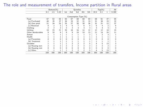
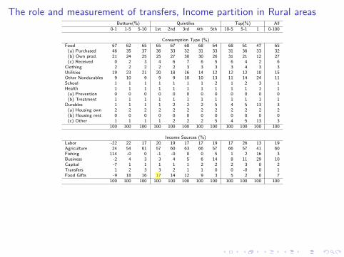
The role and measurement of transfers, Income partition in Rural areasBottom(%) Quintiles Top(%) All
0-1 1-5 5-10 1st 2nd 3rd 4th 5th 10-5 5-1 1 0-100
Consumption Type (%)Food 67 62 65 65 67 68 68 64 68 61 47 65(a) Purchased 46 35 37 36 33 32 31 33 31 36 33 32(b) Own prod. 21 24 25 25 27 30 30 26 31 21 12 27(c) Received 0 2 3 4 6 7 6 5 6 4 2 6
Clothing 2 2 2 2 2 3 3 3 3 4 3 3Utilities 19 23 21 20 18 16 14 12 12 12 10 15Other Nondurables 9 10 9 9 9 10 10 13 11 14 24 11School 1 1 1 1 1 1 1 2 1 2 3 1Health 1 1 1 1 1 1 1 1 1 1 1 1(a) Prevention 0 0 0 0 0 0 0 0 0 0 0 0(b) Treatment 1 1 1 1 1 1 1 1 1 1 1 1
Durables 1 1 1 1 2 2 2 5 4 5 13 3(a) Housing own 2 2 2 2 2 2 2 2 2 2 2 2(b) Housing rent 0 0 0 0 0 0 0 0 0 0 0 0(c) Other 1 1 1 1 2 2 2 5 4 5 13 3
100 100 100 100 100 100 100 100 100 100 100 100
Income Sources (%)Labor -22 22 17 20 19 17 17 19 17 26 13 19Agriculture 24 54 61 57 60 63 66 57 66 57 41 60Fishing 114 -0 0 -1 -0 0 0 5 1 2 16 3Business -2 4 3 3 4 5 6 14 8 11 29 10Capital -7 1 1 1 1 1 2 2 2 3 0 2Transfers 1 2 3 3 2 1 1 0 0 -0 0 1Food Gifts -9 18 16 17 14 12 9 3 5 2 0 7
100 100 100 100 100 100 100 100 100 100 100 100
Wealth Portfolio (%)Housing 50 50 39 38 42 32 27 25 25 27 24 30Other Durables 10 5 4 5 5 6 7 15 11 16 39 9Land 30 38 49 50 46 49 52 36 41 30 21 44Agric. structures 0 0 0 0 0 1 1 1 1 1 1 1Agric. equipment 2 1 1 2 1 2 2 3 3 3 4 2Fishing equipment 1 0 0 0 0 0 0 1 2 0 1 0Livestock 8 6 6 5 5 10 12 20 18 23 11 13Debt -0 -0 -0 -0 -0 -0 -0 -1 -1 -1 -0 -0
100 100 100 100 100 100 100 100 100 100 100 100
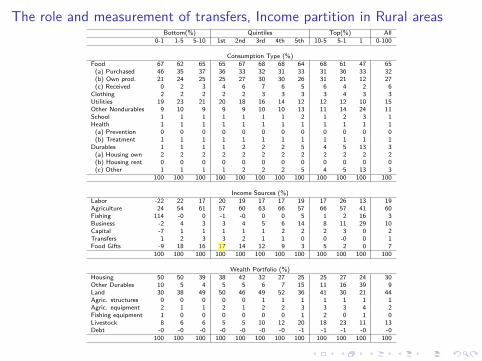
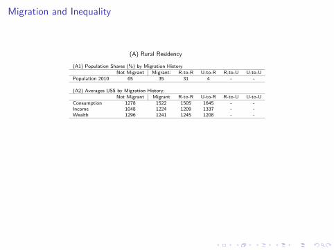
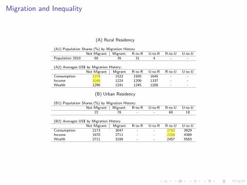
Migration and Inequality
(A) Rural Residency
(A1) Population Shares (%) by Migration HistoryNot Migrant Migrant: R-to-R U-to-R R-to-U U-to-U
Population 2010 65 35 31 4 - -
(A2) Averages US$ by Migration History:Not Migrant Migrant R-to-R U-to-R R-to-U U-to-U
Consumption 1278 1522 1505 1645 - -Income 1048 1224 1209 1337 - -Wealth 1296 1241 1245 1208 - -
(B) Urban Residency
(B1) Population Shares (%) by Migration History:Not Migrant Migrant: R-to-R U-to-R R-to-U U-to-U
22 78 - - 60 18
(B2) Averages US$ by Migration HistoryNot Migrant Migrant R-to-R U-to-R R-to-U U-to-U
Consumption 2173 3047 - - 2782 3929Income 1670 2711 - - 2206 4389Wealth 2711 3180 - - 2457 5583
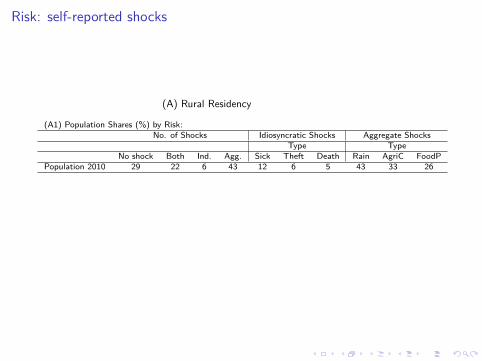
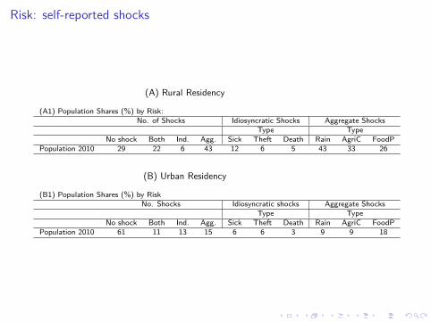
Risk: self-reported shocks
(A) Rural Residency
(A1) Population Shares (%) by Risk:No. of Shocks Idiosyncratic Shocks Aggregate Shocks
Type TypeNo shock Both Ind. Agg. Sick Theft Death Rain AgriC FoodP
Population 2010 29 22 6 43 12 6 5 43 33 26
(B) Urban Residency
(B1) Population Shares (%) by RiskNo. Shocks Idiosyncratic shocks Aggregate Shocks
Type TypeNo shock Both Ind. Agg. Sick Theft Death Rain AgriC FoodP
Population 2010 61 11 13 15 6 6 3 9 9 18
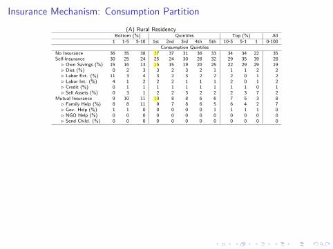
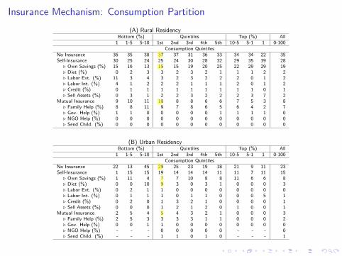
Insurance Mechanism: Consumption Partition(A) Rural Residency
Bottom (%) Quintiles Top (%) All1 1-5 5-10 1st 2nd 3rd 4th 5th 10-5 5-1 1 0-100
Consumption QuintilesNo Insurance 36 35 38 37 37 31 36 33 34 34 22 35Self-Insurance 30 25 24 25 24 30 28 32 29 35 39 28
. Own Savings (%) 15 16 13 15 15 19 20 25 22 29 29 19
. Diet (%) 0 2 3 3 2 3 2 1 1 1 2 2
. Labor Ext. (%) 11 3 4 3 2 3 2 2 2 0 1 2
. Labor Int. (%) 4 1 2 2 2 1 1 1 2 0 1 2
. Credit (%) 0 1 1 1 1 1 1 1 1 1 0 1
. Sell Assets (%) 0 3 1 2 2 3 2 2 2 3 7 2Mutual Insurance 9 10 11 10 8 8 6 6 7 5 3 8
. Family Help (%) 8 8 11 9 7 8 6 5 6 4 2 7
. Gov. Help (%) 1 1 0 0 0 0 0 1 1 1 1 0
. NGO Help (%) 0 0 0 0 0 0 0 0 0 0 0 0
. Send Child. (%) 0 0 0 0 0 0 0 0 0 0 0 0
(B) Urban ResidencyBottom (%) Quintiles Top (%) All1 1-5 5-10 1st 2nd 3rd 4th 5th 10-5 5-1 1 0-100
Consumption QuintilesNo Insurance 22 13 45 29 25 23 19 18 21 9 11 23Self-Insurance 1 15 15 19 14 14 14 11 11 7 11 15
. Own Savings (%) 1 11 4 7 7 10 8 8 11 6 6 8
. Diet (%) 0 0 10 9 3 0 3 1 0 0 0 3
. Labor Ext. (%) 0 2 1 1 0 0 0 0 0 0 0 0
. Labor Int. (%) 0 1 1 1 0 1 1 0 0 0 5 1
. Credit (%) 0 2 0 1 3 2 1 0 0 0 0 1
. Sell Assets (%) 0 0 0 1 2 1 2 0 1 0 0 1Mutual Insurance 2 5 4 5 4 3 2 1 0 0 0 3
. Family Help (%) 2 5 3 3 3 3 1 1 0 0 0 2
. Gov. Help (%) 0 0 1 1 0 0 0 0 0 0 0 0
. NGO Help (%) - - - 0 0 0 0 0 - - - 0
. Send Child. (%) - - - 1 1 0 1 0 - - - 1
Borrowing
I Among rural households, 25% claim they did not need it. Among urbanhouseholds, 33% claim they did not need it.
I Conditional on needing a loan, 40% of urban households ask for one and 27% ofrural households asked for one.
I This shows that urban areas haver better access to borrowing. But are theseloans used to smooth consumption?
I No, the main reason is start-up capital. In urban areas borrowing is used 3.6times more often for start-up capital than for consumption. In rural areas thisnumber is 1.6.
Final Remarks
I Our evidence suggests that households in Malawi are unable to accumulatewealth (relative to the US).
I Despite low wealth accumulation, consumption is being smoothed. Risk sharing isan important mechanism.
I The conjecture that we turn to in future research is whether there is a trade-offbetween low accumulation of wealth and risk sharing.