Cross-document coreference for WePS

Iustin Dornescu, Constantin Orasan and Tatiana Lesnikova

RIILP, University of Wolverhampton, UK{I.Dornescu2,C.Orasan,Tatiana.Lesnikova}@wlv.ac.uk

Abstract. A good clustering performance depends on the quality of thedistance function used to asses similarity. In this paper we propose a pair-wise document coreference model to improve performance over a word-vector similarity approach for the WePS 3 clustering task. We identify asimple criterion which discriminates between highly ambiguous queries,i.e. many small clusters, and balanced queries, i.e. fewer, larger clusters.A document clustering framework was developed facilitating direct com-parison between different parameters, features and algorithms. It usesa unified feature representation to afford a wide variety of clusteringpipelines. Using the predicted coreference likelihood and a simple clus-tering algorithm, we achieve comparable results on the WePS 2 dataset,and competitive performance on the WePS 3 dataset.

1 Introduction

Disambiguating people names in Web search results is an active research area,combining several Natural Language Processing challenges such as cross-documentcoreference, information extraction and document clustering. A good clusteringperformance depends upon the quality of the similarity function used. Most pre-vious work uses a combination of content-based features, e.g. word, bigrams,NEs, and person attributes, e.g. email, date of birth, title, to compute documentsimilarity [1].

The main aim of this study is to use a supervised cross-document coreferenceapproach [2] to improve performance for the WePS clustering task. A pairwisemodel is used to predict the likelihood that two documents refer to the sameperson. A clustering algorithm will then use these predictions to cluster thedocuments. In order to have a better understanding of what works best andwhy, we developed a generic framework for document clustering which allowscomplex pipelines to be built. By sharing the same feature extraction base, directcomparison between different parameters and algorithms is straightforward.

This paper is structured as follows: the generic framework is presented inSection 2. In Section 3 the elements of the processing pipeline are detailed,and a criterion distinguishing the ambiguity of a query is proposed. The threeclustering algorithms are briefly presented in Section 4, and in Section 5 wedetail the experiments and discuss the results.

2 Generic Architecture

In the recent WePS literature, two main approaches can be distinguished whichneed to be accommodated by the framework:

vector-space clustering – documents are represented as a weighted feature vec-tors – points in a high-dimensional space, which are clustered using a pairwisedistance function. Usually the weighting scheme is tf · idf , the distance func-tion is either cosine or euclidean, and the algorithm is single-link hierarchicalagglomerative clustering (HAC). The stopping criterion most commonly usedis a threshold limiting the link distance between the two nearest clusters. Thisvalue is learnt from training data [1].

feature-graph clustering – the document×feature occurrence matrix is used tobuild a support graph which is used to compute a better document similarity.Usually a bipartite graph is built in which document node d is connected tofeature node f if the feature f is extracted from document d. Afterwards, eithera document×document graph is built, with the edges’ weights reflecting thenumber of shared features (e.g. number of paths of length 2 between the twodocuments), or, conversely, a feature×feature graph is built using the commondocuments as support. Based on the clusters identified in this derived graph, thesolution to the initial problem is built [3].

While conceptually different, both these approaches can be abstracted using aunified graph representation: features extracted from the documents are used tobuild a derived graph, its nodes are then clustered and the documents associatedwith each of the clusters are returned. By sharing the same feature extractionalgorithms, weighting schemes, and distance functions, various approaches canbe directly compared, to gain insights into how efficient solutions to the problemcan be built. In the context of Web search, users expect results to be availablein seconds. For this reason, the ultimate aim of this framework is to analysethe trade-off between computational cost and performance benefit of differentapproaches to the WePS clustering task.

The architecture of the framework is presented in Figure 1. In the first stepof the processing pipeline (a), plain text document views are extracted from theHTML files. A view can also employ NLP techniques to extract only some ofthe contents of another view (b), e.g. a set of snippets mentioning the targetperson, or meta data such as keywords, title, author and so on. The second stepis the feature extraction stage (c) when vectors are extracted from documentviews. For each different feature F , a frequency matrix is built (m(di, fj) =how many times feature value fj occurred in document di). The simplest suchfeature consists of tokenizing and extracting content words (tokenization, stopword removal, indexing), while more involved features employ off-the shelf NLPtools and person-data information extraction. Rows from these matrices can bemerged and/or weighted to create feature vectors. Composite features aggregatefeature vectors from other features. Pairwise features reflect the similarity be-tween document pairs, computed as a distance between their feature vectors.

In the next step a derived graph is built either directly from frequency data(feature-graph clustering), or induced by the pairwise distance matrix (vector-space clustering). This graph is clustered using generic algorithms, and then thesolution is built.

View View View

metadata

snippets

extractsconte

nt

b)

pla

in t

ext

feat

ure

s tokens

entities

attributes

doc

x fea

ture

d)

pai

rwise

com

pat

ibili

ty

doc

x d

ocdistance

corelation

machine learning

f)

parse source formatex

trac

tion

a)

feature extraction, weightingc)

pairwise compatibilitye)

build graph/networkg)

clust

erin

gsim

ilarity

Document

clustering algorithms

clusters

clust

er x

doc

Fig. 1: General architecture of the framework

In this paper we investigate whether ML can be used to provide better com-patibility scores rather than afforded by the standard approach which uses cosinesimilarity in a tf · idf weighted vector space. The intuition is that a machinelearning algorithm can employ both content-based similarity and semantic rulesto make better predictions regarding coreference likelihood. For example, shar-ing the same email address is predictive for the coreference relation, while havingdifferent dates of birth entails two distinct persons. Such rules can have prior-ity over the more generic token based similarity measures. However, we need totake into account the complexity of the IE task: the attribute values will be noisy(low precision) and sparse (low recall). Further more, they are not necessarilyunique per document, e.g. several job titles, and could need specialised semanticsimilarity measures to be compared, e.g. email addresses are easier to comparethan job titles.

The IE framework employed is described in Section 3.2, while the clusteringalgorithms are briefly presented in Section 4. The processing steps are sum-marised in Table 1.

3 Feature Extraction Framework

The plain text extracted from the documents (dom.view) was tokenised andindexed using lucene. To extract named entities, a view (NER.view) was imple-mented wrapping the Stanford NER tool [6]. In was suggested [7] that simplyusing capitalisation yields better results, because generic NER tools are usuallytrained on news wire corpora and do not perform as well on noisy web data,therefore we also used this as an alternative feature (cap.view).

To combine both named entities and terminology, a complex analysis toolbased on Wikipedia-Miner2 was used [8]. The tool examines the text of the pageand detects the most relevant Wikipedia articles, based on information such asthe probability of a span s to be a link to an article a and the probability of twoarticles to co-occur in the same Wikipedia document [4]. The process is relatedto topic indexing and to explicit semantic analysis: each document is representedas a vector in a high dimensional space, but instead of words, the dimensionsare unambiguous Wikipedia topics, ranked by their relevance score (wiki.view).

A novel pairwise feature is the longest common substring (LCS) between twotextual views. Documents describing the same person, tend to share some phrasesand sentences, sometimes entire paragraphs. While naively parallel, LCS takestoo much time to be computed at query time on the full text of the documents,but it performed quite well using the smaller snippet.view instead.

3.1 Token-feature weighting

The system which achieved the best official result on WePS 2 [9] showed thatusing a web-scale corpus to have more accurate IDF values helped boost perfor-mance significantly. Therefore we compared two ways of computing IDF : local– only the set of documents for the current query are used (less than 200 doc-uments), and global – all the documents in all WePS corpora are used (around70K documents). To speed up computation, words with DF = 1 were removed.We also considered increasing the DF threshold to see if this yields better re-sults. Figure 2 shows that the difference between the two weighting schemes issignificant.

When DF threshold is increased: document vectors become nil, which isexpected. The immediate implication is that the cosine similarity becomes un-defined. We observed an interesting effect if global IDF is used: frequent wordssuch as home and contact have very low IDF values, thus considerably morefeature vectors become very small (norm less than 10−6) and are practically nil.Table 2 shows the percentage of undefined pairwise cosine values. Usually log

2 http://wikipedia-miner.sourceforge.net

Table 1: Main components of the processing pipelinedocu

men

tvie

ws

dom.text Jericho HTML parser is used to clean HTML and extracttext from the DOM document, then openNLP1 is used tosplit the text into sentences

plain.text the w3m text browser is used to render the files and dumpthe the textual content as displayed on screen

xhtml.view returns a cleaned xhtml version of the HTML filesnippet.view extracts all snippets spanning ws=300 characters before and

after each target mention; overlapping windows are mergedNER.view employs Stanford NER tool to extract named entities from

the underlying viewcapitalization extracts all the capitalised words and/or sequences, a high-

recall NER baseline

docu

men

tfe

atu

res

words standard tokenization and stop word filtering (using apachelucene library) to create a word vector representation for eachdocument

tokens uses only the marked-up entities, e.g. from NER.viewdensification detects most relevant Wikipedia topics using a wikification

service based on Wikipedia Miner [4]; the document is rep-resented as a weighted topic vector

I.E. RegEx-based framework for extracting person-attributes re-quired in Task1b (see Section 3.2); for each attribute, themost likely candidate values are extracted

pair

wis

efe

atu

res

tf · idf weighting the standard weighting scheme for token-based vectors; weexperimented with two different IDF scopes and several DFthresholds

cosine similarity dot product of length normalised vectorsMinkowski most experiments carried out for L2 (euclidean distance)

Jaccard index the overlap between attribute values: J(A,B) = |A∩B||A∪B|

match if the sets share attribute values: m(A,B) = 1⇐⇒ A∩B 6= φ

overlap weighted version of Jaccard:

∑x∈A∩B

wA(x)+wB(x)∑x∈A∪B

wA(x)+wB(x)

ML

Weka toolkit we experimented mainly with rule based classifiers becausethey are fast, granularity can be controlled by pruning andthey also give insights into what works and what does not

clust

erin

g

HAC standard hierarchical agglomerative clustering, using a pair-wise distance matrix and any of the following link types:single, average, mean, complete, adjcomplete; the maximumlink threshold delta is observed in training data;

CC connected components remaining in a graph after removinglinks longer than the threshold

MCL markov clustering [5], a graph clustering algorithm whichis widely used in biology; it uses a parameter inflation (I)which determines the granularity of the clustering; severalfiltering criteria are employed to reduce node degrees beforethe algorithm is run

(a) cosine, minDF=2, global vs. local (b) euclidean, minDF=2, global vs. local

(c) cosine, minDF=20, global vs. local (d) euclidean, minDF=20, global vs. local

Fig. 2: Word-vector weighting and pairwise distance; impact of global IDF andDF threshold on cosine and euclidean measures (red–coreferent, blue–distinct)

smoothing is used to avoid representation errors (we use the default similarityimplementation from Lucene3), but we discovered that queries with many clus-ters tend to have considerably more undefined values than queries with fewerclusters.

Table 2: Proportion of undefined cosine similarities for different DF limits

IDF minDF=2 minDF=5 minDF=10 minDF=15 minDF=20

local 3055 1% 3840 1% 4396 1% 4994 1% 6653 2%global 51943 14% 161604 44% 198633 55% 212035 58% 224715 62%

Previous work suggests that a criterion discriminating between different typesof sets is beneficial. In [7], a simple heuristic that achieves good results is pro-posed: if at least 3 documents from a random sample of 10 documents are coref-erent use all-in-one, otherwise use one-in-one. The criterion is manually evalu-ated and the clustering is not informative, therefore this is yet another baseline.The performance is Fh = 0.71, compared to the two baselines: Faio = 0.60,Foio = 0.39. In [1] it is acknowledged that choosing an individual clusteringthreshold for each set instead of a global value for the entire data achieves ahigh performance F = 0.85. To pick the parameter value for each set an oraclemethod is used which exploits gold standard information that is not available toa normal system. The performance reported serves as a theoretical upper bound.

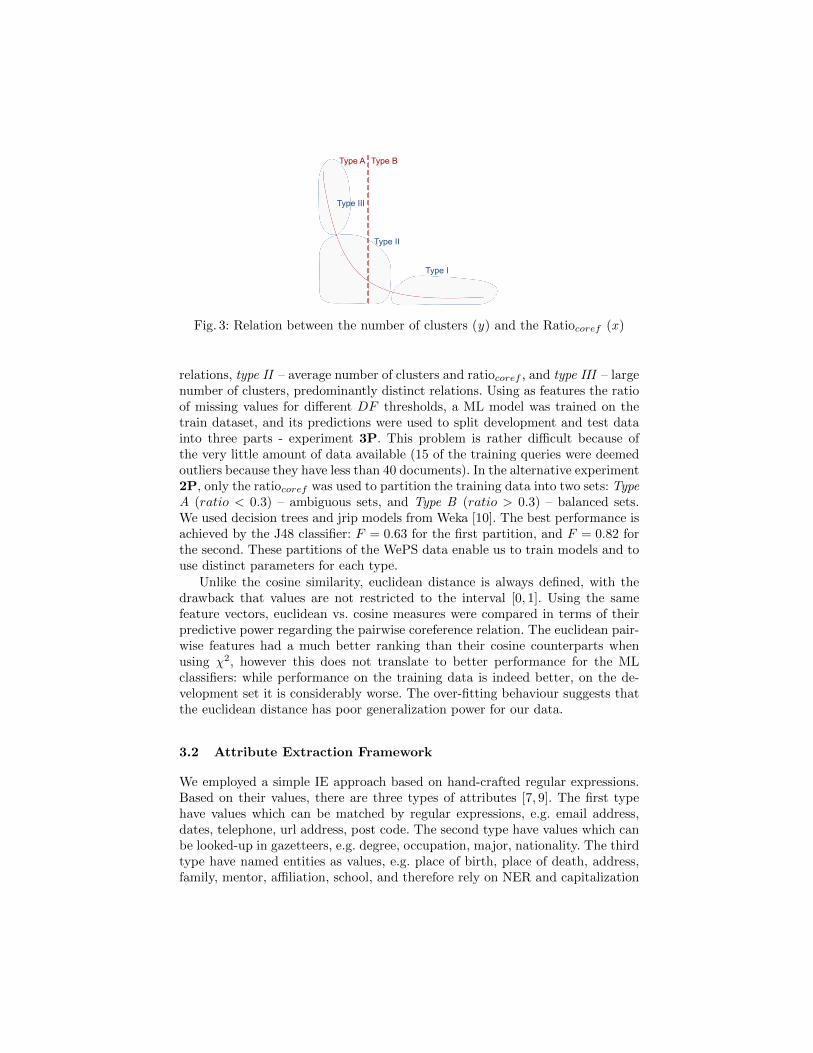
We used gold data to plot each set as a point in a bi-dimensional space(Figure 3): the number of clusters vs. the ratiocoref (the proportion of all pairwiserelations that are coreferent). These points were then clustered using k-means(k=3) yielding 3 types of sets: type I – few clusters and predominantly coreferent

3 http://lucene.apache.org/

Type I

Type II

Type III

Type A Type B

Fig. 3: Relation between the number of clusters (y) and the Ratiocoref (x )

relations, type II – average number of clusters and ratiocoref , and type III – largenumber of clusters, predominantly distinct relations. Using as features the ratioof missing values for different DF thresholds, a ML model was trained on thetrain dataset, and its predictions were used to split development and test datainto three parts - experiment 3P. This problem is rather difficult because ofthe very little amount of data available (15 of the training queries were deemedoutliers because they have less than 40 documents). In the alternative experiment2P, only the ratiocoref was used to partition the training data into two sets: TypeA (ratio < 0.3) – ambiguous sets, and Type B (ratio > 0.3) – balanced sets.We used decision trees and jrip models from Weka [10]. The best performance isachieved by the J48 classifier: F = 0.63 for the first partition, and F = 0.82 forthe second. These partitions of the WePS data enable us to train models and touse distinct parameters for each type.

Unlike the cosine similarity, euclidean distance is always defined, with thedrawback that values are not restricted to the interval [0, 1]. Using the samefeature vectors, euclidean vs. cosine measures were compared in terms of theirpredictive power regarding the pairwise coreference relation. The euclidean pair-wise features had a much better ranking than their cosine counterparts whenusing χ2, however this does not translate to better performance for the MLclassifiers: while performance on the training data is indeed better, on the de-velopment set it is considerably worse. The over-fitting behaviour suggests thatthe euclidean distance has poor generalization power for our data.

3.2 Attribute Extraction Framework

We employed a simple IE approach based on hand-crafted regular expressions.Based on their values, there are three types of attributes [7, 9]. The first typehave values which can be matched by regular expressions, e.g. email address,dates, telephone, url address, post code. The second type have values which canbe looked-up in gazetteers, e.g. degree, occupation, major, nationality. The thirdtype have named entities as values, e.g. place of birth, place of death, address,family, mentor, affiliation, school, and therefore rely on NER and capitalization

to detect possible candidates. The attribute extractors usually check a small win-dow of text around a target entity mention, and use trigger words and phrasesas well as candidate values matcher, i.e. gazetteer, regex, NER. One of the draw-backs of this approach is that it does not make use of automatic bootstrappingalgorithms and that it relies on textual occurrences of attribute values. In thedocument collection more often than not, these attributes are presented in ta-bles. For example, contact details – address, email, url, telephone, fax, and soon, tend to be displayed without mentioning the trigger words we rely on. Inthis case, special extractors are needed which are able to detect several fields atthe same time [9].

Our extraction framework is ill suited for the noisy Web documents. We al-lowed several values to be extracted for the same attribute, and we experimentedwith overlap measures: Jaccard index, a weighted version which uses value fre-quencies, and a simple non-void intersection criterion, i.e. the two documentsmust share at least one attribute value. To our disappointment, the attributefeatures are very sparse.

The attribute features yield mixed results: they are ranked highest usingInformation Gain, but lowest using GainRatio, χ2 ranks them lowest of all. Thissuggests they are too sparse to have a big impact on the overall result, and thatnoise due to inaccurate extraction further limits their utility.

The drawbacks of the IE framework employed make it the biggest limitingfactor for our approach. At the time of writing the final results for Task1b –Attribute Extraction are not yet available.

4 Clustering Algorithms

To perform both vector-space clustering and feature-space clustering, our frame-work represents the pairwise similarity function as a matrix, which also corre-sponds to a weighted graph. This matrix can be computed using arbitrarilycomplex methods, e.g. latent semantic analysis, explicit semantic analysis, butin this case it can only be used with ’stable’ clustering algorithms (e.g. k-medoidsis stable, while k-means is not).

One of the challenges in WePS is that the number of clusters is unknown.Depending on the clustering algorithm employed, the stopping criterion is con-trolled via a parameter which is observed on training data. A quality functionis evaluated at each step of the algorithm. Once this function reaches a criticalpoint the clustering algorithm is stopped.

4.1 Hierarchical agglomerative clustering (HAC)

HAC is one of the most commonly used algorithms due to its simplicity andability to control granularity. The algorithm starts with singleton clusters and,at every step, merges the two nearest clusters. The link distance between twoclusters can be computed in several ways. We investigated five aggregation func-tions (see Table 3). The algorithm stops when only k clusters remain (k is an

Table 3: HAC: link types

SINGLE the minimum distance between documentsAVERAGE the average distance between documentsMEAN the mean distance between documentsCOMPLETE the maximum distance between documentsADJCOMPLETE adjusted complete link using the largest within cluster distance

input parameter) or when the link distance between the two nearest clustersis greater than a threshold delta (another input parameter). In WePS, systemsmainly use the second criterion, selecting the value delta which maximises train-ing performance. We used an implementation based on Weka [10].

4.2 Markov clustering

Markov clustering (MCL) [5] is a general purpose graph clustering algorithmcommonly used in biology. It simulates network flow via two algebraic opera-tions on stochastic matrices. The algorithm stops when convergence is achieved,but the clustering granularity can be controlled via an inflation I parameter.4. Network clustering (community detection) algorithms can benefit from pre-processing the input graph by e.g. removing edges with low similarity [11]. In ourexperiments, removing edges longer than a threshold delta did not have muchimpact on clustering outcome: the output is usually one large cluster. A filter-ing technique which worked well was to limit node degree by keeping the k bestneighbours per node (knn). This technique is common in spectral clustering [11].

4.3 Connected components

The success of single link HAC is intriguing. For the single link delta HAC, noneof the edges with a weight above the threshold are considered by the algorithm,and can thus be removed. Intuitively, the clusters found will correspond to theconnected components of the rest of the graph. We also used a connected com-ponents algorithm (CC) to investigate how it compares to the single link HACimplementation. To our surprise, the results of the two algorithms were different,with the CC algorithm achieving the best performance in most cases.

5 Experiments and Findings

To build the coreference models, WePS 1 data was used for training (6346 doc-uments, 70 queries), WePS 2 data was used for parameter tuning – developmentdata (3444 documents, 30 queries) and the WePS 3 data was used for test (57357

4 mcl version 10-324, http://www.micans.org/mcl/

documents, 300 queries). When the gold standard for WePS 3 became available,it was used to search for the best clustering parameters on the WePS 3 data.

To compare the content similarity approach with the ML coreference ap-proach, we ran three main experiments. In the first experiment (wiki), we usedthe cosine similarity between vectors produced by Wikipedia Miner (wiki.view).In the second experiment (3P) we split the data into 3 parts as described inSection 3.1. A pairwise coreference model was trained for each part, using aset of over 50 pairwise features. The third experiment is similar, only this timewe use the second partitioning method to split data into 2 parts. The sameset of features was used to train the pairwise coreference models, but this timemore pruning was employed, to avoid over-fitting and to obtain better confidencescores for the rules learnt. The pairwise features use a combination of parame-ters: document view, IDF type, DF limit and similarity measure, as well as theoverlap between person attributes.

5.1 Using Wikipedia topics for semantic similarity (wiki)

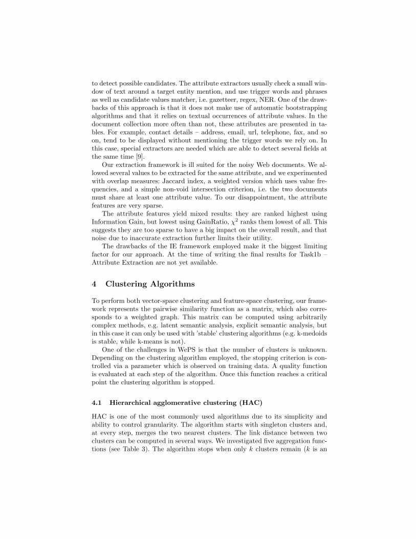
There are significant differences between the different WePS corpora and theirrespective evaluation methodologies. This explains to a certain extent the dropin performance for all WePS 3 participants. Results in figures 4 and 5 show thatHAC has different behaviour on the test data than on the development data:single-link HAC drops from best to worst, while for three of the link types per-formance is almost constant in WePS3, regardless of the delta threshold. Thisis most likely due to the larger number of documents in each query: up to fourtimes more document pairs per query in WePs 3 compared to WePS 1. Thesimple CC clustering is the best performer on both data sets, and has consis-tent behaviour, in both cases reaching maximum F score for delta ∈ [0.7, 0.8].The first official run, Wolves1, used single link HAC with delta = 77, but onlyachieved average performance in the competition.

5.2 Pairwise coreference model (3P)

The number of clusters and their sizes vary greatly from query to query. Whilethe pairwise similarity values are usually within the [0, 1] interval, their distribu-tion seems to be very query-specific. Training a ML model on the entire datasetyielded low performance due to the noisy features. For this reason we appliedthe criterion from Section 3.1.

When training the decision trees classifiers, while good classification accuracywas achieved for types I and III, the kappa statistic was rather low. Our initialexperiments with selecting the delta threshold individually for each set did notimprove performance much. The fact that the maximum score remains almostconstant for most threshold values suggests that the evaluation measures needto be adjusted to account for chance, in order to better reflect performance.

The size difference between test, 200 documents per query, and development,100-150 documents per query, affects the performance of MCL: in development,for low knn it creates many singleton clusters while for values over 90 it creates

0 0.1 0.2 0.3 0.4 0.5 0.6 0.7 0.8 0.9 1

0

0.1

0.2

0.3

0.4

0.5

0.6

0.7

0.8

0.9

1

delta HAC (wiki)

AVERAGESINGLECOMPLETEADJCOMPLETEMEAN

delta threshold

F0

.5

0 0.2 0.4 0.6 0.8 1

0

0.2

0.4

0.6

0.8

1

CC clustering (wiki)

BEPBERF0.5RI

delta threshold

0 0.2 0.4 0.6 0.8 1

0

0.1

0.2

0.3

0.4

0.5

0.6

0.7

0.8

0.9

1

delta HAC

AVERAGESINGLECOMPLETEADJCOMPLETEMEAN

delta threshold

F0

.5

0 0.2 0.4 0.6 0.8 1

0

0.1

0.2

0.3

0.4

0.5

0.6

0.7

0.8

0.9

1

delta HAC - SINGLE

BEPBERF0.5RI

delta threshold

0 0.2 0.4 0.6 0.8 1

0

0.1

0.2

0.3

0.4

0.5

0.6

0.7

0.8

0.9

1

delta HAC - SINGLE

BEPBERF0.5RI

delta threshold

0 0.2 0.4 0.6 0.8 1

0

0.1

0.2

0.3

0.4

0.5

0.6

0.7

0.8

0.9

1

delta HAC - AVERAGE

BEPBERF0.5RI

delta threshold

0 0.2 0.4 0.6 0.8 1

0

0.2

0.4

0.6

0.8

1

delta HAC - ADJCOMPLETE (wiki)

BEPBERF0.5RI

delta threshold

Fig. 4: wiki experiment: performance on the development set

0 0.2 0.4 0.6 0.8 1

0.3

0.32

0.34

0.36

0.38

0.4

0.42

0.44

HAC (wiki)

SINGLEAVERAGECOMPLETEADJCOMPLETEMEAN

delta threshold

0 0.2 0.4 0.6 0.8 1

0

0.2

0.4

0.6

0.8

1

CC clustering (wiki)

BEPBERF0.5

delta threshold

0 0.2 0.4 0.6 0.8 1

0

0.2

0.4

0.6

0.8

1

delta HAC - SINGLE (wiki)

BEPBERF0.5

delta threshold

0 0.2 0.4 0.6 0.8 1

0

0.2

0.4

0.6

0.8

1

delta HAC - AVERAGE (wiki)

BEPBERF0.5

delta threshold

0 0.1 0.2 0.3 0.4 0.5 0.6 0.7 0.8 0.9

0

0.2

0.4

0.6

0.8

1

delta HAC - ADJCOMPLETE (wiki)

BEPBERF0.5

delta threshold

Fig. 5: wiki experiment: performance on the test set

one large cluster; on test data, MCL only reaches the best performance for higherthresholds. The second official run, Wolves2, used group average HAC, but forthe selected delta threshold, it performed poorly on test data. Again, CC clus-tering outperforms both group average HAC and single link HAC on test data.This suggests that using a set of high precision rules can achieve competitiveperformance. Theoretically, for a query with n documents and c clusters, a setof n− c coreferent edges is enough to build the complete clustering solution. Afuture direction of research is to use sampling and weighting approaches to trainhigh precision–low recall models.

0 0.2 0.4 0.6 0.8 1

0

0.2

0.4

0.6

0.8

1

delta HAC (3P)

SINGLEAVERAGECOMPLETEMEANADJCOMPLETE

delta threshold

F0

.5

0 20 40 60 80 100 120 140 160

0

0.2

0.4

0.6

0.8

1

MCL (3P)

I=1.6I=1.8I=2.0I=2.2I=3.0I=3.5

knn filter

F0

.5

0 0.1 0.2 0.3 0.4 0.5 0.6 0.7 0.8

0

0.2

0.4

0.6

0.8

1

CC clustering (3P)

BEPBERF0.5RI

delta threshold

0 0.2 0.4 0.6 0.8 1

0

0.2

0.4

0.6

0.8

1

delta HAC - AVERAGE (3P)

BEPBERF0.5RI

delta threshold

0 20 40 60 80 100 120 140 160

0

0.2

0.4

0.6

0.8

1

MCL (3P) I=3.0

BEPBERF0.5RI

knn filter

0 0.2 0.4 0.6 0.8 1

0

0.2

0.4

0.6

0.8

1

delta HAC -SINGLE (3P)

BEPBERF0.5RI

delta threshold

Fig. 6: 3P experiment: performance on the development set

0 0.2 0.4 0.6 0.8 1

0

0.2

0.4

0.6

0.8

1

delta HAC (3P)

SINGLEAVERAGECOMPLETEADJCOMPLETEMEAN

delta threshold

0 10 20 30 40 50 60 70 80 90

0

0.2

0.4

0.6

0.8

1

MCL (3P)

I=1.6I=1.8I=2.0I=2.2I=3.0I=3.5

knn filter

0 0.2 0.4 0.6 0.8

0

0.2

0.4

0.6

0.8

1

CC clustering (3P)

BEPBERF0.5

delta threshold

0 0.2 0.4 0.6 0.8 1

0

0.2

0.4

0.6

0.8

1

delta HAC - AVERAGE (3P)

BEPBERF0.5

delta threshold

0 10 20 30 40 50 60 70 80 90

0

0.2

0.4

0.6

0.8

1

MCL (3P) - I=3.0

BEPBERF0.5

knn filter0 0.2 0.4

0

0.2

0.4

0.6

0.8

1

delta HAC- SINGLE (3P)

BEPBERF0.5

delta threshold

Fig. 7: 3P experiment: performance on the test set

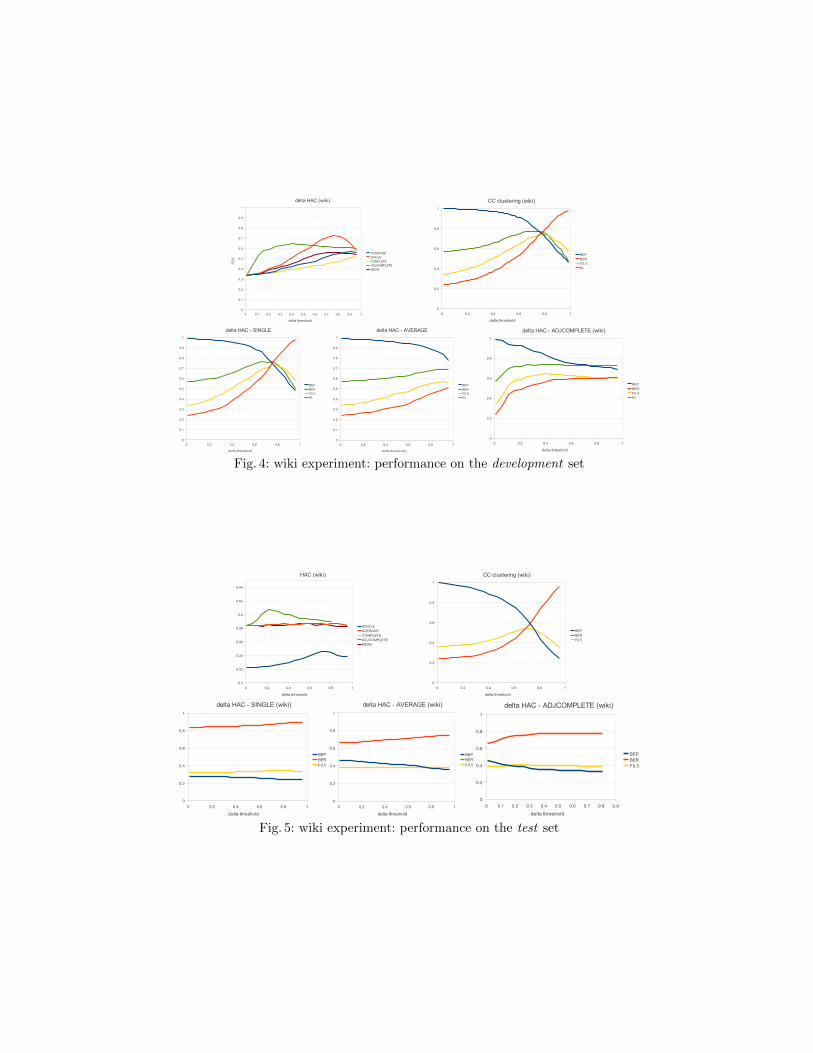
5.3 Pairwise coreference model (2P)

This experiment was designed to investigate whether the low performance ob-tained by the Wolves2 run is due to over-fitting. Training data was split only intwo larger sets, and pruning was increased for the J48 classifiers, from 100 to1000 minimum covered instances. This experiment achieves the best results, butit revealed that the clustering threshold influenced performance.

0 0.2 0.4 0.6 0.8 1

0

0.2

0.4

0.6

0.8

1

delta HAC (2P)

SINGLEAVERAGECOMPLETEADJCOMPLETEMEAN

delta threshold

0 10 20 30 40 50 60 70 80 90

0

0.2

0.4

0.6

0.8

1

MCL (2P)

I=1.6I=1.8I=2.0I=2.2I=3.0I=3.5

knn filter

0 0.2 0.4 0.6 0.8 1

0

0.2

0.4

0.6

0.8

1

CC clustering (2P)

BEPBERF0.5RI

delta threshold

0 0.2 0.4 0.6 0.8 1

0

0.2

0.4

0.6

0.8

1

delta HAC - AVERAGE (2P)

BEPBERF0.5RI

delta threshold

0 10 20 30 40 50 60 70 80 90 100

0

0.2

0.4

0.6

0.8

1

MCL (2P) - I=3.0

BEPBERF0.5RI

knn filter0 0.2 0.4 0.6 0.8 1

0

0.2

0.4

0.6

0.8

1

delta HAC - SINGLE (2P)

BEPBERF0.5RI

delta threshold

Fig. 8: 2P experiment: performance on the development set

0 0.2 0.4 0.6 0.8 1

0

0.2

0.4

0.6

0.8

1

delta HAC (2P)

SINGLEAVERAGECOMPLETEADJCOMPLETEMEAN

delta threshold

0 10 20 30 40 50 60 70 80 90

0

0.2

0.4

0.6

0.8

1

MCL (2P)

I=1.6I=1.8I=2.0I=2.2I=3.0I=3.5

knn filter

0 0.2 0.4 0.6 0.8 1

0

0.2

0.4

0.6

0.8

1

CC clustering (2P)

BEPBERF0.5

delta threshold

0 0.2 0.4 0.6 0.8 1

0

0.2

0.4

0.6

0.8

1

delta HAC - AVERAGE (2P)

BEPBERF0.5

delta threshold

0 10 20 30 40 50 60 70 80 90

0

0.2

0.4

0.6

0.8

1

MCL (2P) - I=3.0

BEPBERF0.5

knn filter0 0.2 0.4 0.6 0.8 1

0

0.2

0.4

0.6

0.8

1

delta HAC- SINGLE

BEPBERF0.5

delta threshold

Fig. 9: 2P experiment: performance on the test set

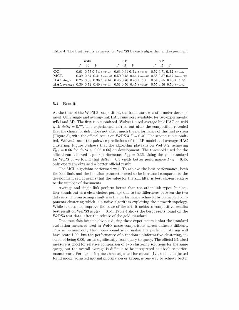
Table 4: The best results avhieved on WePS3 by each algorithm and experiment

wiki 3P 2PP R F P R F P R F

CC 0.61 0.57 0.54 δ=0.71 0.63 0.61 0.54 δ=0.15 0.52 0.71 0.52 δ=0.21

MCL 0.39 0.54 0.41 knn=90 0.50 0.48 0.44 knn=50 0.58 0.57 0.52 knn=125

HACsingle 0.25 0.88 0.36 δ=0.76 0.45 0.70 0.48 δ=0.11 0.54 0.55 0.48 δ=0.16

HACaverage 0.39 0.72 0.40 δ=0.71 0.51 0.50 0.45 δ=0.46 0.55 0.56 0.50 δ=0.61

5.4 Results

At the time of the WePS 3 competition, the framework was still under develop-ment. Only single and average link HAC runs were available, for two experiments:wiki and 3P. The first run submitted, Wolves1, used average link HAC on wikiwith delta = 0.77. The experiments carried out after the competition revealedthat the choice for delta does not affect much the performance of this first system(Figure 5), with the official result on WePS 3 F = 0.40. The second run submit-ted, Wolves2, used the pairwise predictions of the 3P model and average HACclustering. Figure 6 shows that the algorithm plateaus on WePS 2, achievingF0.5 = 0.66 for delta ∈ [0.06, 0.66] on development. The threshold used for theofficial run achieved a poor performance F0.5 = 0.36. Using the gold-standardfor WePS 3, we found that delta = 0.5 yields better performance F0.5 = 0.45;only one team obtained a better official result.

The MCL algorithm performed well. To achieve the best performance, boththe knn limit and the inflation parameter need to be increased compared to thedevelopment set. It seems that the value for the knn filter is best chosen relativeto the number of documents.

Average and single link perform better than the other link types, but nei-ther stands out as a clear choice, perhaps due to the differences between the twodata sets. The surprising result was the performance achieved by connected com-ponents clustering which is a naive algorithm exploiting the network topology.While it does not improve the state-of-the-art, it achieves competitive results:best result on WePS3 is F0.5 = 0.54. Table 4 shows the best results found on theWePS3 test data, after the release of the gold standard.

One issue that became obvious during these experiments is that the standardevaluation measures used in WePS make comparisons across datasets difficult.This is because only the upper-bound is normalised: a perfect clustering willhave score 1.00, but the performance of a random uninformative clustering, in-stead of being 0.00, varies significantly from query to query. The official BCubedmeasure is good for relative comparison of two clustering solutions for the samequery, but the overall average is difficult to be interpreted as absolute perfor-mance score. Perhaps using measures adjusted for chance [12], such as adjustedRand index, adjusted mutual information or kappa, is one way to achieve better

Table 5: WePS3 official results

System avg. BCubed precision avg. BCubed recall avg. F-measure

YHBJ 2 unofficial 0.61 0.6 0.55AXIS 2 0.69 0.46 0.5WOLVES 1 0.31 0.8 0.4WOLVES 2 0.26 0.88 0.36one in one baseline 1 0.23 0.35all in one baseline 0.22 1 0.32

understanding of what works for WePS and how well it works. Another concernis that the WePS3 evaluation methodology, by considering documents split intothree clusters – person A, person B and other, differs significantly from the ini-tial task formulation. This makes it even more difficult to determine if a systemwith very high performance on WePS 3 data will perform similarly on real lifedata, when more then two clusters, if not all, are evaluated.

Future work will focus on extending the IE framework and on adding feature-space clustering algorithms which achieve state-of-the-art performance on WePS2.Mining high precision rules exploiting semantic attributes will also be investi-gated, as recall seems to be less important. Another model which will be inves-tigated is to consider pairwise relation as coreferent, undecided and distinct.

6 Conclusions

This paper reports the experiments carried out for the WePS3 clustering task.A generic framework was developed allowing the implementation and compar-ison of varied clustering pipelines. We compared a similarity-based approachin a Wikipedia-topic space representation with two rule-based ML coreferencemodels trained on pairwise document similarity measures. We showed that asimple clustering algorithm can exploit high precision predictions of the pair-wise coreference model, achieving comparable performance on WePS 2 datasetand competitive performance on the WePS 3 dataset.

References

1. Artiles, J., Gonzalo, J., Sekine, S.: Weps 2 evaluation campaign: overview of theweb people search clustering task. In: 2nd Web People Search Evaluation Workshop(WePS 2009), 18th WWW Conference. (2009)

2. Bagga, A., Baldwin, B.: Entity-based cross-document coreferencing using the vec-tor space model. In: COLING-ACL. (1998) 79–85

3. Jiang, L., Wang, J., An, N., Wang, S., Zhan, J., Li, L.: Grape: A graph-basedframework for disambiguating people appearances in web search. IEEE Interna-tional Conference on Data Mining (2009) 199–208

4. Milne, D., Witten, I.H.: Learning to link with Wikipedia. In: CIKM ’08: Proceedingof the 17th ACM conference on Information and knowledge management, NewYork, NY, USA, ACM (2008) 509–518

5. van Dongen, S.: Graph Clustering by Flow Simulation. PhD thesis, University ofUtrecht (2000)

6. Finkel, J.R., Grenager, T., Manning, C.: Incorporating non-local information intoinformation extraction systems by gibbs sampling. In: ACL ’05: Proceedings of the43rd Annual Meeting on Association for Computational Linguistics, Morristown,NJ, USA, Association for Computational Linguistics (2005) 363–370

7. Lan, M., Zhang, Y.Z., Lu, Y., Su, J., Tan, C.L.: Which who are they? peopleattribute extraction and disambiguation in web search results. In: 2nd Web PeopleSearch Evaluation Workshop (WePS 2009), 18th WWW Conference. (2009)

8. Medelyan, O., Legg, C., Milne, D., Witten, I.H.: Mining Meaning from Wikipedia.Computing Research Repository (CoRR) (2008)

9. Chen, Y., Lee, S.Y.M., Huang, C.R.: Polyuhk: A robust information extractionsystem for web personalnames. In: 2nd Web People Search Evaluation Workshop(WePS 2009), 18th WWW Conference. (2009)

10. Hall, M., Frank, E., Holmes, G., Pfahringer, B., Reutemann, P., Witten, I.H.: Theweka data mining software: an update. SIGKDD Explor. Newsl. 11(1) (2009)10–18

11. von Luxburg, U.: A tutorial on spectral clustering. CoRR abs/0711.0189 (2007)12. Vinh, N.X., Epps, J., Bailey, J.: Information theoretic measures for clusterings

comparison: is a correction for chance necessary? In: ICML ’09: Proceedings of the26th Annual International Conference on Machine Learning, New York, NY, USA,ACM (2009) 1073–1080