Embed Size (px)
Citation preview

Crop Price Indemnified Loans for Farmers:
A Pilot Experiment in Rural Ghana
Dean Karlan
Yale University
Innovations for Poverty Action
MIT Jameel Poverty Action Lab
Ed Kutsoati
Tufts University
Margaret McMillan
Tufts University
National Bureau of Economic Research
Chris Udry
Yale University
November 10, 2010
* The authors thank USAID/BASIS, Tisch College of Tufts University, and the Bill and
Melinda Gates Foundation via the Financial Access Initiative for funding; the Institute of
Economic Affairs (IEA-Ghana) for support and hospitality; seminar participants at the
BASIS conference sponsored by the University of Wisconsin, Richard Philipps and
participants at the 5th
International Microinsurance Conference sponsored by the
Microinsurance Network and Munich Re Foundation; Kelly Bidwell, Angeli Kirk, Jake
Mazar, Justin Oliver, and Elana Safran from Innovations for Poverty Action for field
research support; Doug Randall and Jesse Gossett from Tufts University for field
research assistance and the management team at Mumuadu Rural Bank.
All opinions herein are our own and not those of any of the donors.

Crop Price Indemnified Loans for Farmers:
A Pilot Experiment in Rural Ghana
Abstract: Farmers face a particular set of risks that complicate the decision to borrow.
We use a randomized experiment to investigate 1) the role of crop-price risk in reducing
demand for credit among famers and 2) how risk mitigation changes farmers’ investment
decisions. In rural Ghana, we offer farmers loans with an indemnity component that
forgives 50% of the loan if crop-prices drop below a threshold price. A control group is
offered a standard loan product at the same interest rate. We find similarly high loan
uptake among all farmers and little significant impact of the indemnity component on
uptake or other outcomes of interest, with the exception of higher likelihoods of garden
egg cultivation and sales to market traders rather than at farmgate among indemnified
loan recipients.
Key words: agricultural credit, crop prices, crop price insurance, underinvestment, impact
evaluation, clustered randomized control trial

2
Farmers face a particular set of risks that complicate the decision to borrow. Factors that are almost
entirely unforeseeable and outside of their control, such as crop prices and weather patterns, have an
enormous impact on farmers’ fortunes – and on their ability to repay any loans they have taken. As such,
some farmers are believed reluctant to take loans to finance seemingly profitable ideas for fear of not
being able to repay. Paradoxically, from a bank’s perspective, these may be excellent clients. They are
so trustworthy that they are not borrowing out of fear of default. Can a loan product with a component
that mitigates farmers’ risk successfully encourage farmers to take, and benefit from, credit? What type
of individuals are more likely to borrow when some of the risk is mitigated? And lastly but equally
importantly, how does the mitigation of risk change farmers’ investment decisions, such as the purchase
of inputs?
Most of the theoretical literature on the impact of credit constraints on productivity focuses on
supply side constraints. In a recent departure, Boucher, Carter and Guirkinger (2005) argue that in the
presence of moral hazard, farmers will prefer not to borrow even though the loan would raise their
productivity and expected income. Using panel data from Peru, they identify these “risk rationed” (as
opposed to quantity rationed) households as households who never tried to access the formal market
because of the high risk associated with borrowing due to consequences of default, and show that risk
rationing adversely affects the productivity of these households. Based on this they argue that
improvements in the insurance offered to these households would increase their willingness to
participate in formal credit markets and raise household welfare.
As farmers weigh their ability to generate sufficient crop revenue to repay loans, one of the primary
risks they face is price variability, which can be very high between and within growing seasons. In terms
of price risk management, Morgan (2001) reviews the literature on reducing price risk through support
and stabilization measures (e.g., International Commodity Agreements). Price support – often through

3
marketing boards – has been a common but generally unsustainable policy. Because of the risks and
politics involved in maintaining international boards, there has been a broad trend to liberalize
agricultural markets, shifting price risk onto producers and traders, and furthermore the boards typically
are only setup for dominant export crops.
Due to these difficulties with International Commodity Agreements, Morgan (1999, 2001) outlines
theoretical justification for the demand for futures markets and other risk-management tools in
developing countries but suggests that few systems are implemented successfully in practice, due to
frequently-unsatisfied infrastructural requirements.
Although in theory the most efficient approach, futures markets are not readily available for many
farmers and crops, in particular for farmers in developing countries. Carter (1999) surveys the literature
on reducing price variability through derivatives such as futures and options markets. Such markets
remain relatively uncommon in developing countries, however, and even where they exist, they are
primarily accessible to large-volume producers and traders rather than smallholder farmers (Varangis
and Larson 1996).
Carter (1999) in particular points to evidence that farmers in developed countries seem to hedge their
price risk less than would appear to be optimal and again emphasizes a striking lack of evidence on their
counterparts in developing countries. Attempting to begin filling this gap, a comparative study by
Woolverton (2007) interviewing US and South African farmers suggests that in the absence of price
supports, farmers do show a higher demand for price-risk reduction strategies, though Jordaan and
Grove (2007) find that demand may be tempered by distrust of the market and insufficient education.
These studies seem to focus more on larger-scale farmers who may also be less credit-constrained. There
is still very little empirical evidence on how smallholders in particular respond to price-risk management
products.

4
We are unaware of any crop price insurance offered to smallholder farmers, but recent efforts to sell
rainfall insurance are highly instructive. Giné and Yang (2007) study whether the inclusion of rainfall
insurance (at marginal cost) into a loan product induces farmers to borrow. To their surprise, loan take-
up was actually lower by 13 percentage points among farmers that had to buy insurance along with the
loan. They also find that take-up of the insured loan is positively correlated with education while take-up
of the uninsured loan is not. Thus it is clear that inclusion of insurance in loans (in that case, at
actuarially fair prices plus a load to cover insurance company costs) for smallholders is not necessarily
an easy task that generates higher demand for the loan.
To investigate whether price risk affected the demand for credit, we conducted a simple social
experiment in which some loans included a crop price indemnification clause (a “natural field
experiment” in the taxonomy put forward by Harrison and List, 2004). Mumuadu Rural Bank in the
Eastern Region of Ghana, in conjunction with Innovations for Poverty Action, offered credit to farmers
to invest in their farms. Mumuadu conducted marketing meetings to groups of maize and garden egg
(eggplant) farmers. Randomly assigned, in half of the meetings farmers were offered the opportunity to
apply for loans that included crop price indemnification at no additional charge, i.e., if crop prices fell
below a certain floor during the harvest time, 50% of their loan was forgiven. In the other half of the
meetings (control), farmers were offered a normal loan, with repayment required irrespective of future
crop prices. Farmers attending both sets of meetings merely knew that the bank was holding a meeting
to talk about credit in their community; they were not told that there was variation in the types of loans
being offered.1 By not disclosing to farmers that there was a randomized trial within the lending
program, the experiment avoids concerns of “randomization bias,” that only certain types of individuals
are prone to participate in randomized trials (Heckman 1992). Indeed, this social experiment was
1 We cannot, however, rule out the possibility that farmers may have known each other across groups.
5
entirely “natural” (Harrison and List, 2004) in that, aside from the surveying, the individuals interacted
with the bank and saw themselves as clients of the bank.
By conducting this as a randomized control trial, we address two general endogeneity problems.
First, those who choose to participate in insurance programs are likely different than those who do not
(e.g., more risk averse, perhaps more entrepreneurial or resourceful in finding good financial solutions to
their problems), and second, those who are approved typically by lenders are different than those who
are not. Note that although the take-up rates of the loans was 86% in the control and 92% in the
treatment groups, our analysis of impacts is done on the intent to treat basis, i.e., everyone offered
treatment loans are analyzed as part of the treatment group (and not just the self-selected sample of those
who take-up), and the same for the control group.
There are two important methodological points to note. First, the possibility exists that there was
learning across the two groups of farmers given the social ties that likely exist between farmers living in the
same village. In particular, if one farmer finds out that his neighbour has been offered a loan on more
favourable terms than herself, she might be less likely to take up the “normal” loan. However, since take up
rates are quite similar across both types of loans we do not think that this type of learning had an impact on
our results. Furthermore, no anecdotal reports of complaints or queries were made to the bank, thus
reinforcing the belief that contagion effects were unlikely to have occurred. Second, as with any data
collection process, one must always point out that those who participate in a process, whether it be a
research process or some other intake process, may be different than the general population. In this case,
since participants did not perceive their participation as part of a research project but rather as a process to
potentially get a loan, the issue is simply that these results may not apply to individuals with no interest in
receiving credit from a rural bank for agriculture.

6
Two additional issues that come up in the context of natural field experiments are recruitment bias and
the possibility of learning across treatment and control groups. It is well known that recruitment bias could
significantly contaminate the results of a field trial like ours and that the direction of bias would be difficult
to pin down a priori. However, since subjects were not paid to participate in our experiment, we do not
think that recruitment bias is especially important in our case. Finally, the possibility exists that there was
learning across the two groups of farmers given the social ties that likely exist between farmers living in the
same village. In particular, if one farmer finds out that his neighbour has been offered a loan on more
favourable terms than herself, she might be less likely to take up the “normal” loan. However, since take up
rates are quite similar across both types of loans we do not think that this type of learning had an impact on
our results.
II. Loan Product Description and Rationale
7
Our choice of loan product was initially based on focus group meetings with farmers and Bank
management. In these meetings, farmers reported that one reason they were not borrowing from
Mumuadu Bank was fear of default in the event that prices collapse. Opinion from Bank management
also suggested this was a significant risk. Several further factors made indemnification of crop prices a
good candidate for the product. First, more than half of farmers interviewed in a baseline survey said
they would be willing to pay to guarantee a floor for the price of their crop. Furthermore, rainfall, an
alternative risk commonly discussed, does not vary enough in this region of Ghana to be considered a
substantial risk for most farmers (Keyzer et al. 2007), but crop prices do vary considerably. Finally, crop
prices are determined in centralized local markets and are thus outside any individual farmer’s control or
likely influence. Data on these prices are collected by government officials and are easily and quickly
verifiable.
The Mumuadu Bank loan product was simple. If the price of the farmer’s crop (either maize or
garden egg) at the time of harvest fell below a given level (set to be at the 10th
percentile of historical
garden egg prices during harvest period and at the 7th
percentile of historical year-long prices for maize),
then Mumuadu Bank forgave 50% of the principal and interest of the farmers’ loan. To set the crop price
levels and choose the crops, we gathered data from the Ghana Ministry of Agriculture and engaged in
conversations with Ministry of Agriculture extension agents, farmers, and Mumuadu Rural Bank. We
chose the two crops – garden eggs (eggplant) and maize – due to their prevalence in the region, their
price volatility, and availability of historical data. Farmers attended the meetings already in groups
designating them as either garden egg or maize, and there was no opportunity to switch crops afterwards
depending on prices or other factors.
The loan with crop price indemnification aims to encourage investment, and thus the key outcome
measure, beyond take-up of the loan, is whether investment behavior changed for the farmers. We have

8
three sources of data: a baseline survey, the administrative data from the bank with regard to take-up and
repayment, and a follow-up survey that focused on investment decisions of the farmers.
III. Experimental Design
The project launched in August 2007. Mumuadu Bank employees contacted key community
members (district assemblyman, storekeepers, farmers) in each of five villages to collect the names of
all maize and garden egg (eggplant) farmers in the village. From the listing, farmers were randomly
assigned into either the control or treatment group, and the same community members invited the
farmers to marketing meetings separated by treatment and control.
At the beginning of each of the marketing meetings, Mumuadu employees explained that the
bank was doing marketing research on farmers in the area, and then asked the farmers to participate in a
baseline survey. Table 1 presents the summary statistics from this baseline survey for those who were
also successfully reached in the follow-up survey, one year later. Appendix Table 1 presents the
summary statistics from the baseline survey for everyone surveyed in the baseline, and compares those
means to those also found for the follow-up, in order to assess whether there was any noticeable attrition
pattern. All statistics include farmers who were offered loans, regardless of whether or not they chose to
apply later. The aggregate test finds that those who were found for the follow-up survey were
systematically different (F-statistic = 1.84, p-value = 0.028). The attrition bias seems driven mostly by
those who perceived price risk to be higher, those who prefer to borrow from banks over relatives, and
maize farmers (all three groups were more likely to be found for the follow-up survey). Because attrition
is non-negligible in our sample, a series of robustness checks have been added to the estimation section
and are presented in Appendix Tables 2, 3, and 4. Results appear to be robust to a correction for
attrition.

9
Once the baseline survey was complete in the meetings, one of four credit officers from
Mumuadu Bank then presented the loan offer to the group of farmers. A total of 169 farmers attended
one of the 20 meetings. Of these 169, 91 were maize farmers and 78 were garden egg (eggplant)
farmers. Farmers were not informed that the bank was offering two different products; rather, the bank
simply offered the treatment group their loan offer, and offered the control group the loan without the
crop price indemnification.
Farmers then had one month to apply for a loan. Loans were disbursed about one month after
application; between September 13th
and October 17th
for maize farmers, and between November 17th
and December 13th
for garden egg farmers. Average loan size is 238 GHS (or 159 USD), which
represents a large change in cash flow - roughly 13-38 percent of the typical farmer’s average annual
income. A follow-up survey was conducted after 2-3 crop cycles (roughly one year), to determine the
impact of the indemnified loan on input usage and investment.
IV. Data and Analysis2
The survey instrument for the pilot contains 28 questions and is primarily designed to measure
basic demographic information plus data on loan history and plans, cognitive ability, risk perception and
aversion, and financial management skills. The survey instrument is available upon request.
We begin with an analysis of differences in means. Our first goal is to verify that the
randomization generated observably similar treatment and control groups. Table 1 Column 4 shows the
t-statistics for a series of comparison of means, which all showed that the treatment assignment was
orthogonal to all key observable variables collected in the baseline survey. The joint test of all covariates
(F-stat = 0.75, p-value = 0.74 reported in the notes) also shows that the randomization successfully
generated observable similar treatment and control groups jointly.
2 The dataset and estimate code are available on the Innovations for Poverty Action website.

10
Next, we are interested in comparing the characteristics of those who apply for the standard loan
to the characteristics of those who apply for the indemnified loan. For instance, are those who are more
risk averse more likely to borrow with the indemnified loan? Or perhaps the price indemnification is
difficult to understand, and thus those with higher cognitive abilities or education are more likely to take
it up, relative to a simple loan. Ideally we would know the riskiness of different farmers (which perhaps
is proxied by their risk aversion), in order to test a model of adverse selection versus advantageous
selection (note that we employed hypothetical survey questions to measure risk preferences, rather than
incentivized questions as done in, e.g., Harrison et al 2010).
Table 1 columns 5 through 13 show, via comparison of means, what types of individuals were
more likely to take-up the loan overall (columns 5-7), under the control condition (columns 8-10), and
the treatment condition (columns 11-13). Overall, farmers who borrowed were roughly 6 years older
than farmers who did not borrow, their cognitive scores were almost one full point (out of 7) higher,
they were twice as likely to have borrowed previously, especially from a financial institution, and they
were somewhat more ambiguity averse.
Then Table 2 shows similar results using probit econometric specifications:
,)1( iiiiiii TXXTA
where Ai is an indicator variable equal to 1 if the individual takes up a loan. Ti is an indicator variable
for assignment to the treatment group – the farmers who get marketed the indemnified loan. Xi is a
vector of demographic and other survey responses, and i is an error term for farmer i, which allowed
for clustering at the group (i.e., meeting) level.
We find very few differences in take-up. Any heterogeneity is likely masked by the large take-up
rates for both: 86% in control group and 92% in treatment group (the difference is not statistically
significant) took-up a loan. We do not find a difference in take-up due to cognitive score or prior

11
experience borrowing, but we do find that those who believed that prices were likely to fall were less
likely to take-up the treatment loan than the control loan.3 This was significant at the 90% level. Our
prior was the opposite: the loan protects farmers from prices falling, and thus those who believe prices
will fall will have higher demand for crop price protection. The reversal of this we find interesting and
puzzling. We posit one story, ex-post: the survey question picked up pessimism4 in general, not just
pessimism with respect to crop prices, and pessimistic individuals were skeptical of the indemnified loan
product.
Next, in Table 3 (summary statistics and mean comparisons) and Table 4 (probit and tobit
specifications)5, we estimate the impact of the indemnified loan on investment and profits using the first
difference estimator obtained by comparing the levels of the outcome variables between the treatment
and control groups. To avoid self-selection bias related to farmers’ decisions to apply for a loan, we
estimate the intent-to-treat impact – the impact of being offered a price-indemnified loan regardless of
take-up.
Table 4 uses the following econometric specification:
,)2( iiiii XTY
where Yi is the outcome of interest, and Xi is a vector of baseline covariates that are not included in
Columns 1 and 2 and included in Columns 3 and 4. We use tobit estimation for non-negative continuous
variables and probit for binary variables. Due to the randomization, the first difference estimator
provides an unbiased estimate of the impact of the indemnified loan on investment and profits, without
risk of endogeneity with respect to who decided to take-up or who was offered credit by the bank.
3 The question asked was, “In your view, what is the likelihood that the price of 27kg of garden eggs will fall below 70,000
between January and April?” Respondents could answer on a scale of 1 to 3 from very unlikely to very likely, and this is
summed with the response to the same question asked about the next five years. A similar question was asked of maize
farmers. 4 “Pessimism” is meant here in a layman’s sense rather than a formal one.
5 OLS results are available from the authors, and are not qualitatively different.
12
We find that farmers offered the indemnified loans spent on average 23.1 percentage points
(significant at 90%, but not significant when not including control variables) more on chemicals for their
primary crop as a share of the total spent on chemical inputs. Other than this, there is no indication that
the indemnified loan had an impact on investment in inputs.
We also see a shift towards growing garden eggs by 17.5 percentage points (significant at 95% in
specifications with baseline control variables, not significant in specifications without baseline controls
but the point estimate is similar) and harvesting less maize, resulting in a decrease of 270 kg of maize
harvested (significant at 95%). As garden eggs are the more perishable and thus potentially riskier crop,
although both were protected by the indemnification clause, the relative reduction in risk was greater for
garden eggs.
We find a potentially interesting result regarding how and when farmers marketed their crop.
Note that the indemnified loan was not conditional on the price that they received for their crop, but
rather on the average price in the area at the time of harvest. Farmers were 18% more likely to sell their
crops to market traders, rather than to farmgate sellers who come to them and pick up the crop.
Anecdotal evidence suggests that the farmgate sellers offer contracts which lock in prices, but at lower
prices. Those willing to risk market prices are typically rewarded on average. Two further pieces of
information would have helped tell a complete story, but we do not have them. First, if this
interpretation is correct, historical price data at the farmgate should be lower and less volatile than
historical price data at the market. Second, we should be able to document that farmgate buyers are
indeed locking in prices for farmers before harvest. Lastly, default was large, with 58% of borrowers (no
difference between treatment and control) in default as of May 2009.
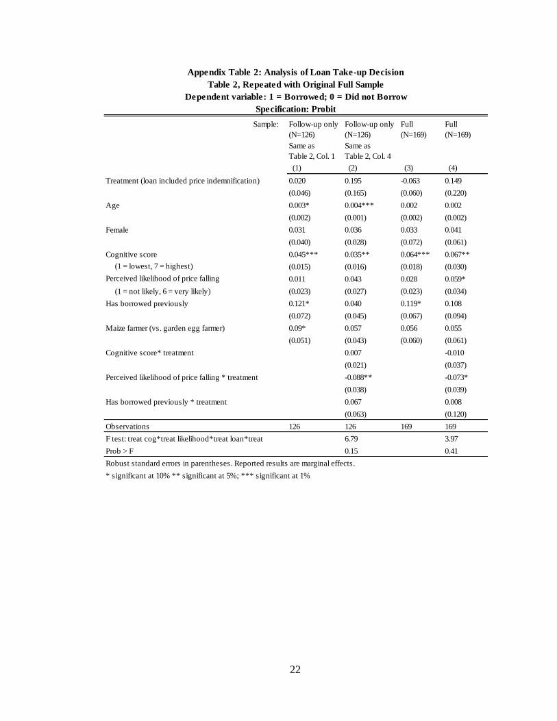
Given the attrition (126 out of 169 farmers successfully surveyed for the follow-up), Appendix
Tables 2 and 3 show estimates on borrowing outcomes on both the final sample who could be reached

13
for interview during the follow-up (i.e., same as in the primary tables) as well as for the full original
sample. Appendix Table 4 reports results of estimating equation (2) using inverse probability weighting
to correct for attrition. To obtain the weights, we run a probit regression of attrition on control variables
plus those variables that distinguish attriters as determined in Appendix Table 1. The results in Table 4
are robust to this attrition correction.
V. Discussion and Directions for Future Research
Ironically, the surprisingly high take-up rate of credit made it difficult to assess heterogeneity in
take-up that the study aimed to test. We specifically designed this product to be built-in to the loan,
rather than as an add-on insurance. This, combined with the fact that the triggering event was measured
by the Ministry of Agriculture, reduced the processing costs for the Bank. We also integrated the
insurance with the loan to avoid potential choice overload problems (i.e., when too many choices cause
stagnation in decision-making, see Bertrand et al. (2010) and Iyengar and Lepper (2000)). Giné and
Yang (2007) also discuss this issue (and related issues of confusion that the insurance may generate to
those unfamiliar with insurance) in a working paper version of their rainfall insurance experiment, in
which take-up rates for credit plus rainfall insurance were lower than take-up rates for credit alone (in
their case, the rainfall insurance was priced at actuarially fair prices plus a load).6 How to ensure that
farmers truly understand such a product is a larger question which can be explored through further
empirical research.
Due to the high take-up rates and thus little room for heterogeneity in take-up, we focus our
attention on the impact, or lack thereof in significant ways, on farmer decisions. A few factors may be at
work to generate few impacts. First, did farmers fully understand the indemnity clause? Priced fairly, the
product undoubtedly makes financial sense for many farmers; by investing more in their crops they are
6 Giné and Yang (2007) is the working paper version of Giné and Yang (2009).

14
more likely to earn increased farm income, and this product lowered the risk they faced with such
investments. Second, perhaps one year is not enough time. The farmers needed to believe that the crop
price indemnification loans would be offered for years to come in order to start making large investment
changes. Third, the high rates of default we observe may indicate that the bank already effectively had in
place a flexible "loan forgiveness" program, so the additional indemnification had little impact on
behavior. Lastly, it could be that the crop prices were simply not causing that much volatility for
farmers. Observed crop prices may have been volatile, and may have been the focus of much attention,
but through storage and optimal timing of sales farmers are able to mitigate this risk at least partially on
their own. Related to this, a study by Mahul (2000) suggests that farmers may jointly consider price and
yield risk. It is possible that the impact of reducing price risk may be muted in the presence of
unmitigated yield risk. Lastly, sample size of the study was small, and thus many of the results were
positive but not significant statistically. In many of the cases, we are not able to rule out large and
meaningful results.
This experiment tried to address a key question for development: does risk inhibit investment.
Although many interventions try to mitigate risk by selling insurance or loans at market prices, the even
simpler question remains: if the risk were removed, without any selection effects, how would behavior
change? We tried to answer this through the simplest way possible: to give away the crop price
indemnification rather than sell it (and thus only observe the intent to treat effect on those who want
their crop price risk mitigated). We see this approach as enlightening, to in a sense know how high the
bar can be for the impact of insurance on investment. Further research needs to be done on other risks
(e.g., rainfall), with larger sample sizes, and perhaps with training and longer term commitments to
maintain a presence in a market.

15
References Cited
Bertrand, Marianne, Dean Karlan, Sendhil Mullainathan, Eldar Shafir, and Jonathan Zinman (2010).
“What’s Advertising Content Worth? Evidence from a Consumer Credit Marketing Field
Experiment,” Quarterly Journal of Economics 125(1), forthcoming.
Boucher, Steve, Michael R. Carter, and Catherine Guirkinger (2008). “Risk Rationing and Wealth
Effects in Credit Markets: Theory and Implications for Agricultural Development,” American
Journal of Agricultural Economics, 90(2), May, 409-423.
Carter, Colin (1999). “Commodities futures markets: a survey,” The Australian Journal of Agricultural
and Resource Economics, 43(2), 209-247.
Giné, Xavier and Dean Yang (2007). “Insurance, Credit, and Technology Adoption: Field Experimental
Evidence from Malawi,” World Bank Policy Research Working Paper Series, December 1.
Giné, Xavier and Dean Yang (2009). “Insurance, Credit, and Technology adoption: Field Experimental
Evidence from Malawi,” Journal of Development Economics, 89(1), May, 1-11.
Harrison, Glenn, Humphrey Steven, and Arjan Verschoor (2010). “Choice Under Uncertainty: Evidence
from Ethiopia, India and Uganda,” Journal of Economic Behavior and Organization, 120 (543),
80-104.
Harrison, Glenn and John List (2004). “Field Experiments,” Journal of Economic Literature, 42(4),
1009-1055.
Heckman, James (1992). "Randomization and Social Policy Evaluation," in Charles Manski and Irwin
Garfinkel: Evaluating Welfare and Training Programs. Cambridge and London: Harvard
University Press, 201-30.
Iyengar, Sheena and Mark Lepper (2000). “When Choice is Demotivating: Can One Desire Too Much
of a Good Thing?” Journal of Personality and Social Psychology 79(6), December, 995-1006.
Jordaan, H and B Grové (2007). “Factors Affecting Maize Producers Adoption of Forward Pricing in
Price Risk Management: The Case of Vaalharts,” Agrekon, 46(4), December, 548.
Keyzer, Michiel, Vasco Molini and Bart van den Boom (2007). “Risk minimizing index functions for
price-weather insurance, with application to rural Ghana,” Center for World Food Studies SOW-
VU Working Paper 07-02.
Mahul, Olivier (2000). “Crop Insurance under Joint Yield and Price Risk,” The Journal of Risk and
Insurance, 67(1), March, 109-122.

16
Morgan, C.W. (2001). “Commodity futures markets in LDCs: a review and prospects,” Progress in
Development Studies, 1(2), 139–150
Morgan, C.W., Rayner, A.J. and Vaillant, C. (1999). “Agricultural futures markets in LDCs: a policy
response to price volatility?” Journal of International Development 11, 893–910.
Varangis, Panos and Larson, Don (1996) . “Dealing with commodity price uncertainty,” Policy
Research Working Paper 1167. Washington, DC: World Bank International Economics
Department, World Bank.
Woolverton, Andrea (2007). Institutional effects on grain producer price-risk management behavior: a
comparative study across the United States and South Africa. Dissertation, University of
Missouri-Columbia.

17
Reached for
Follow-up Survey
(N=126)
Control
(N=66)
Treatment
(N=60)
No
(N=14)
Yes
(N=112)
No
(N=9)
Yes
(N=57)
No
(N=5)
Yes
(N=55)
(1) (2) (3) (5) (6) (8) (9) (11) (12)
Age 43.413 44.394 42.333 0.903 37.929 44.098 1.716 * 34.111 46.018 2.765 *** 44.800 42.109 0.440
(1.138) (1.552) (1.677) (3.563) (1.191) (2.831) (1.646) (8.267) (1.697)
Female 0.151 0.121 0.183 0.969 0.143 0.152 0.087 0.111 0.123 0.098 0.200 0.182 0.099
(0.032) (0.040) (0.050) (0.097) (0.034) (0.111) (0.044) (0.200) (0.052)
Number of dependents 5.992 6.348 5.600 1.422 4.929 6.125 1.431 4.778 6.596 1.582 5.200 5.636 0.358
(0.264) (0.399) (0.335) (0.715) (0.282) (0.969) (0.430) (1.114) (0.353)
Education score 4.135 4.045 4.233 0.464 4.143 4.134 0.014 4.333 4.000 0.411 3.800 4.273 0.439
(0 = no schooling, 9 = highest) (0.201) (0.277) (0.295) (0.686) (0.211) (0.866) (0.293) (1.241) (0.305)
Cognitive score 4.643 4.500 4.800 1.240 3.929 4.732 2.114 ** 3.889 4.596 1.514 4.000 4.873 1.344
(1 = lowest, 7 = highest) (0.121) (0.162) (0.181) (0.355) (0.127) (0.484) (0.170) (0.548) (0.189)
Ambiguity aversion score 2.310 2.242 2.383 1.007 1.929 2.357 1.949 * 2.111 2.263 0.512 1.600 2.455 2.595 **
(1 = not averse, 3 = very averse) (0.070) (0.101) (0.095) (0.322) (0.067) (0.423) (0.099) (0.510) (0.089)
Do you have health insurance? 0.532 0.485 0.583 1.103 0.500 0.536 0.251 0.333 0.509 0.971 0.800 0.564 1.018
(0.045) (0.062) (0.064) (0.139) (0.047) (0.167) (0.067) (0.200) (0.067)
Taken any loan 0.595 0.591 0.600 0.103 0.357 0.625 1.938 * 0.444 0.614 0.954 0.200 0.636 1.934 *
(0.044) (0.061) (0.064) (0.133) (0.046) (0.176) (0.065) (0.200) (0.065)
Taken loan from financial institution 0.325 0.273 0.383 1.322 0.071 0.357 2.174 ** 0.111 0.298 1.166 0.000 0.418 1.864 *
(0.042) (0.055) (0.063) (0.071) (0.045) (0.111) (0.061) (0.000) (0.067)
Prefer to borrow from bank, not relative 0.841 0.848 0.833 0.231 0.929 0.830 0.944 0.889 0.842 0.359 1.000 0.818 1.036
(0.033) (0.044) (0.049) (0.071) (0.036) (0.111) (0.049) (0.000) (0.052)
Would use loan to buy farm inputs 0.952 0.924 0.983 1.558 1.000 0.946 0.883 1.000 0.912 0.916 1.000 0.982 0.299
(0.019) (0.033) (0.017) (0.000) (0.021) (0.000) (0.038) (0.000) (0.018)
Perceived likelihood of price falling 2.548 2.576 2.517 0.322 2.429 2.563 0.460 2.000 2.667 1.744 * 3.200 2.455 1.678 *
(1=not likely, 6 = very likely) (0.091) (0.133) (0.125) (0.309) (0.096) (0.333) (0.142) (0.490) (0.127)
Maize farmer (vs. garden egg farmer) 0.579 0.591 0.567 0.273 0.500 0.589 0.634 0.444 0.614 0.954 0.600 0.564 0.154
(0.044) (0.061) (0.065) (0.139) (0.047) (0.176) (0.065) (0.245) (0.067)
Number of crops planned 1.968 1.970 1.967 0.018 1.786 1.991 0.786 2.111 1.947 0.465 1.200 2.036 2.137 **
(0.082) (0.120) (0.111) (0.334) (0.083) (0.484) (0.119) (0.200) (0.116)
Planned to grow maize at baseline 0.643 0.682 0.600 0.953 0.643 0.643 0.000 0.667 0.684 0.103 0.600 0.600 0.000
(0.043) (0.058) (0.064) (0.133) (0.045) (0.167) (0.062) (0.245) (0.067)
Planned to grow gegg at baseline 0.452 0.424 0.483 0.661 0.500 0.446 0.377 0.556 0.404 0.849 0.400 0.491 0.383
(0.045) (0.061) (0.065) (0.139) (0.047) (0.176) (0.066) (0.245) (0.068)
(4)
Decision to Apply: Control Decision to Apply: TreatmentDecision to ApplyRandomization
T-stat
(2)<>(3)
T-stat
(5)<>(6)
T-stat
(8)<>(9)
T-stat
(11)<>(12)
General:
Lending History:
Farming:
Joint F-test of significance for selection into the treatment group: 0.75, p-value: 0.740
Standard errors in parentheses. * significant at 10%, ** significant at 5%; *** significant at 1%
Table 1: Baseline Summary Statistics: Orthogonality Verification and Take-up Analysis
Baseline Means and Standard Errors
(13)(10)(7)

18
Probit Probit (25th Percentile) Probit (75th Percentile) Probit
(1) (2) (3) (4)
Treatment (loan included price indemnification) 0.020 0.002 0.000 0.195
(0.046) (0.004) (0.000) (0.165)
Age 0.003* 0.000* 0.000* 0.004***
(0.002) (0.000) (0.000) (0.001)
Female 0.031 0.004 0.000 0.036
(0.040) (0.005) (0.000) (0.028)
Cognitive score 0.045*** 0.003*** 0.000*** 0.035**
(1 = lowest, 7 = highest) (0.015) (0.001) (0.000) (0.016)
Perceived likelihood of price falling 0.011 0.001 0.000 0.043
(1 = not likely, 6 = very likely) (0.023) (0.002) (0.000) (0.027)
Has borrowed previously 0.121* 0.102** 0.000** 0.040
(0.072) (0.050) (0.000) (0.045)
Maize farmer (vs. garden egg farmer) 0.09* 0.051* 0.000* 0.057
(0.051) (0.030) (0.000) (0.043)
Cognitive score* treatment 0.007
(0.021)
Perceived likelihood of price falling * treatment -0.088**
(0.038)
Has borrowed previously * treatment 0.067
(0.063)
Observations 126 126 126 126
F test: treat cog*treat likelihood*treat loan*treat 6.79
Prob > F 0.15
Table 2: Analysis of Loan Take-up Decision
Dependent variable: 1 = Borrowed; 0 = Did not Borrow
Probit Results
Robust standard errors in parentheses. Reported results are marginal effects.
* significant at 10% ** significant at 5%; *** significant at 1%
Significant coefficients in column (3) are smaller than 0.001

19
Overall
(N=126)
Control
(N=66)
Treatment
(N=60)
(1) (2) (3)
Applied for loan 0.889 0.864 0.917 0.942
(0.028) (0.043) (0.036)
Loan principal (GHS), borrowers only 238.4 239.6 237.2 0.187
(6.24) (9.41) (8.26)
Loan principal (GHS), all obs 182.94 180.30 185.83 0.272
(10.11) (14.40) (14.27)
Had overdue balance in May 2009, borrowers only 0.516 0.500 0.533 0.371
(0.045) (0.062) (0.065)
Had overdue balance in May 2009, all obs 0.586 0.579 0.593 0.145
(0.047) (0.066) (0.067)
Cultivated indemnity crop 0.778 0.742 0.817 0.997
(0.037) (0.054) (0.050)
Cultivated garden egg 0.254 0.182 0.333 1.966 *
(0.039) (0.048) (0.061)
Cultivated maize 0.738 0.773 0.700 0.923
(0.039) (0.052) (0.060)
Amount of land farmed in minor season (acres) 2.567 2.773 2.342 1.562
(0.139) (0.190) (0.201)
Amount of land farmed: indemnity crop (acres) 2.147 2.288 1.992 0.712
(0.207) (0.338) (0.229)
Used certified seed on indemnity crop, growers only 0.490 0.449 0.531 0.803
(0.051) (0.072) (0.072)
Used certified seed on indemnity crop, all obs 0.381 0.333 0.433 1.151
(0.043) (0.058) (0.065)
Total spent on chemicals for indemnity crop (GHS) 54.795 60.670 48.333 0.941
(6.546) (11.451) (5.513)
Total spent on chems for indemnity crop, % all crops 0.679 0.604 0.762 1.990 **
(0.040) (0.058) (0.054)
Total labor days used 36.722 33.833 39.900 0.719
(4.208) (3.947) (7.719)
Total labor days used on indemnity crop 26.373 25.742 27.067 0.209
(3.160) (3.954) (5.045)
Amount harvested from garden egg crop (kg), growers only424.333 485.909 388.684 0.323
(142.709) (138.181) (213.247)
Amount harvested from garden egg crop (kg), all obs 101.032 80.985 123.083 0.563
(37.233) (31.529) (70.337)
Amount harvested from maize crop (kg), growers only 464.690 529.441 384.146 1.246
(58.135) (88.593) (68.969)
Amount harvested from maize crop (kg), all obs 339.298 409.114 262.500 1.594
(46.226) (73.639) (52.392)
Revenue for all crops (GHS), all obs 309.250 346.045 268.775 0.930
(41.452) (65.037) (49.659)
Sold indemnity crop, growers only 0.929 0.939 0.918 0.389
(0.026) (0.035) (0.040)
Sold indemnity crop, all obs 0.722 0.697 0.750 0.660
(0.040) (0.057) (0.056)
Sold indemnity crop to market trader, growers only 0.440 0.348 0.533 1.795 *
(0.052) (0.071) (0.075)
Sold indemnity crop to market trader, all obs 0.317 0.242 0.400 1.910 *
(0.042) (0.053) (0.064)
Table 3: Outcome Summary Statistics
Mean and Standard Errors
Standard errors in parentheses. * significant at 10%, ** significant at 5%; *** significant at 1%.
"Indemnity crop" refers to maize for the maize group and garden eggs for the garden egg group.
T-stat
(2)<>(3)
(4)
Borrowing:
Sales and Income:
Cultivation and Inputs:

20
Specification:
Includes baseline covariates:
Applied for loan 0.053 0.030
(0.061) (0.048)
Loan principal (GHS) 7.667 6.644
(30.673) (26.762)
Had overdue balance in May 2009, borrowers only 0.014 0.034
(0.125) (0.137)
Had overdue balance in May 2009, all obs 0.033 0.052
(0.126) (0.131)
Cultivated indemnity crop 0.074 0.088
(0.142) (0.072)
Cultivated garden egg 0.152 0.175 **
(0.147) (0.081)
Cultivated maize -0.073 -0.070
(0.146) (0.074)
Amount of land farmed in minor season (acres) -0.423 -0.422
(0.332) (0.350)
Amount of land farmed: indemnity crop (acres) -0.179 -0.075
(0.683) (0.489)
Used certified seed on indemnity crop, growers only 0.082 0.086
(0.110) (0.118)
Used certified seed on indemnity crop, all obs 0.100 0.115
(0.102) (0.091)
Total spent on chemicals for indemnity crop (GHS) -4.35 -4.17
(28.72) (24.44)
Total spent on chems for indemnity crop, % all crops 0.212 0.231 *
(0.220) (0.118)
Total labor days used 6.918 5.587
(10.709) (9.690)
Total labor days used on indemnity crop 4.073 4.358
(13.019) (9.573)
Amount harvested from garden egg crop (kg) 282.28 417.62
(662.35) (560.28)
Amount harvested from maize crop (kg) -257.30 ** -270.35 **
(128.40) (121.70)
Revenue for all crops (GHS) -97.99 -106.16
(104.97) (82.00)
Sold indemnity crop -0.020 -0.061
(0.074) (0.102)
Sold indemnity crop to market trader, growers only 0.186 0.254 **
(0.117) (0.115)
Sold indemnity crop to market trader, all obs 0.158 0.185 *
(0.111) (0.103)
Table 4: Treatment Effects
Dependent Variables: Each row represents a different dependent variable
Marginal effects presented for probit and Tobit results. Probits used for binary indicators
and Tobits for non-negative continuous variables. Robust standard errors in parentheses.
* significant at 10%, ** significant at 5%, *** significant at 1%. Control variables for
column (2) are age, female, education, cognitive score, ambiguity aversion, perceived
likelihood of price drop, and maize farmer (vs. garden egg group). 'Indemnity crop' is maize
for the maize farmer group and garden eggs for the garden egg group.
Probit/Tobit
Yes
(2)
Probit/Tobit
No
(1)
Sales and Income:
Cultivation and Inputs:
Borrowing:

21
Full Sample
Interviewed at
Baseline
(N=169)
Interviewed at
Baseline Only
(N=43)
Reached for
Follow-up
Survey
(N=126)
(1) (2) (3)
Treatment: Selected for crop price indemnity 0.509 0.605 0.476 1.455
(0.039) (0.075) (0.045)
Age 42.905 41.419 43.413 0.908
(0.957) (1.735) (1.138)
Female 0.166 0.209 0.151 0.888
(0.029) (0.063) (0.032)
Number of dependents 5.840 5.395 5.992 1.156
(0.225) (0.428) (0.264)
Education score 4.254 4.605 4.135 1.219
(0 = no schooling, 9 = highest) (0.168) (0.294) (0.201)
Cognitive score 4.609 4.512 4.643 0.547
(1 = lowest, 7 = highest) (0.104) (0.206) (0.121)
Ambiguity aversion score 2.260 2.116 2.310 1.365
(1 = not averse, 3 = very averse) (0.062) (0.130) (0.070)
Do you have health insurance? 0.538 0.558 0.532 0.298
(0.038) (0.077) (0.045)
Taken any loan 0.592 0.581 0.595 0.159
(0.038) (0.076) (0.044)
Taken loan from financial institution 0.325 0.326 0.325 0.002
(0.036) (0.072) (0.042)
Prefer to borrow from bank, not relative 0.811 0.721 0.841 1.745 *
(0.030) (0.069) (0.033)
Would use loan to buy farm inputs 0.964 1.000 0.952 1.458
(0.014) (0.000) (0.019)
Perceived likelihood of price falling 2.414 2.023 2.548 2.941 ***
(1=not likely, 6 = very likely) (0.079) (0.147) (0.091)
Maize farmer (vs. garden egg farmer) 0.538 0.419 0.579 1.833 *
(0.038) (0.076) (0.044)
Number of crops planned 2.030 2.209 1.968 1.496
(0.070) (0.135) (0.082)
Planned to grow maize at baseline 0.627 0.581 0.643 0.717
(0.037) (0.076) (0.043)
Planned to grow gegg at baseline 0.485 0.581 0.452 1.462
(0.039) (0.076) (0.045)
Joint F-test of significance on being surveyed at follow-up: 1.84, p-value: 0.028
* significant at 10%, ** significant at 5%; *** significant at 1%.
Farming:
Lending History:
General:
T-stat
(2)<>(3)
(4)
Appendix Table 1: Analysis of Attrition
22
Sample: Follow-up only
(N=126)
Follow-up only
(N=126)
Full
(N=169)
Full
(N=169)
Same as
Table 2, Col. 1
Same as
Table 2, Col. 4
(1) (2) (3) (4)
Treatment (loan included price indemnification) 0.020 0.195 -0.063 0.149
(0.046) (0.165) (0.060) (0.220)
Age 0.003* 0.004*** 0.002 0.002
(0.002) (0.001) (0.002) (0.002)
Female 0.031 0.036 0.033 0.041
(0.040) (0.028) (0.072) (0.061)
Cognitive score 0.045*** 0.035** 0.064*** 0.067**
(1 = lowest, 7 = highest) (0.015) (0.016) (0.018) (0.030)
Perceived likelihood of price falling 0.011 0.043 0.028 0.059*
(1 = not likely, 6 = very likely) (0.023) (0.027) (0.023) (0.034)
Has borrowed previously 0.121* 0.040 0.119* 0.108
(0.072) (0.045) (0.067) (0.094)
Maize farmer (vs. garden egg farmer) 0.09* 0.057 0.056 0.055
(0.051) (0.043) (0.060) (0.061)
Cognitive score* treatment 0.007 -0.010
(0.021) (0.037)
Perceived likelihood of price falling * treatment -0.088** -0.073*
(0.038) (0.039)
Has borrowed previously * treatment 0.067 0.008
(0.063) (0.120)
Observations 126 126 169 169
F test: treat cog*treat likelihood*treat loan*treat 6.79 3.97
Prob > F 0.15 0.41
Appendix Table 2: Analysis of Loan Take-up Decision
Specification: Probit
Table 2, Repeated with Original Full Sample
Dependent variable: 1 = Borrowed; 0 = Did not Borrow
Robust standard errors in parentheses. Reported results are marginal effects.
* significant at 10% ** significant at 5%; *** significant at 1%

23
Specification: Probit/Tobit Probit/Tobit
Sample: Follow-up only
(N=126)
Full
(N=169)
Same as
Table 4, Col. 2
(1) (2)
Applied for loan 0.030 -0.059
(0.048) (0.061)
Loan principal (GHS) 6.644 29.180
(26.762) (28.951)
Had overdue balance in May 2009, borrowers only 0.034 0.038
(0.137) (0.092)
Had overdue balance in May 2009, all obs 0.052 0.069
(0.131) (0.098)
Borrowing and repayment information were collected as part of Mumuadu's
administrative data, so data were available for all 169 individuals. The results with the
final sample of 126 are presented to keep a sample consisent with the follow-up
outcomes. Control variables for column are age, female, education, cognitive score,
ambiguity aversion, perceived likelihood of price drop, and maize farmer (vs. garden
egg group). Robust standard errors in parentheses. * significant at 10%, ** significant
at 5%, *** significant at 1% (No results are significant).
Borrowing:
Appendix Table 3: Treatment Effects
Table 4, Panel A: Repeated with Original Full Sample
Specifications: Probit/Tobit with Baseline Covariates

24
Specification:
Sample:
Includes baseline covariates:
Cultivated indemnity crop 0.074 -0.033 0.088 -0.007
(0.142) (0.099) (0.072) (0.032)
Cultivated garden egg 0.152 0.085 0.175 ** 0.050
(0.147) (0.116) (0.081) (0.052)
Cultivated maize -0.073 -0.068 -0.070 -0.014
(0.146) (0.116) (0.074) (0.028)
Amount of land farmed in minor season (acres) -0.423 -0.499 -0.422 -0.507
(0.332) (0.362) (0.350) (0.383)
Amount of land farmed: indemnity crop (acres) -0.179 -0.772 -0.075 -0.831
(0.683) (0.520) (0.489) (0.567)
Used certified seed on indemnity crop, growers only 0.082 0.273 0.086 0.251
(0.110) (0.177) (0.118) (0.203)
Used certified seed on indemnity crop, all obs 0.100 0.226 0.115 0.223
(0.102) (0.188) (0.091) (0.186)
Total spent on chemicals for indemnity crop (GHS) -4.35 11.09 -4.17 0.34
(28.72) (21.31) (24.44) (18.29)
Total spent on chems for indemnity crop, % all crops 0.212 0.231 0.231 * 0.188
(0.220) (0.237) (0.118) (0.119)
Total labor days used, all obs 6.918 -16.477 5.587 -11.424
(10.709) (14.607) (9.690) (9.316)
Total labor days used on indemnity crop, all obs 4.073 -17.754 4.358 -10.042
(13.019) (17.649) (9.573) (9.990)
Amount harvested from garden egg crop (kg), all obs 282.28 282.88 417.62 252.95
(662.35) (714.40) (560.28) (488.81)
Amount harvested from maize crop (kg), all obs -257.30 ** -410.72 ** -270.35 ** -390.60 **
(128.40) (168.87) (121.70) (152.54)
Revenue for all crops (GHS), all obs -97.99 -169.00 -106.16 -150.51 *
(104.97) (132.89) (82.00) (84.49)
Sold indemnity crop, growers only -0.020 -0.012 -0.061 -0.083
(0.074) (0.102) (0.102) (0.093)
Sold indemnity crop to market trader, growers only 0.186 0.066 0.254 ** 0.150
(0.117) (0.225) (0.115) (0.173)
Sold indemnity crop to market trader, all obs 0.158 0.037 0.185 * 0.091
(0.111) (0.194) (0.103) (0.141)
Cultivation and Inputs:
Sales and Income:
Marginal effects presented for probit and tobit results. Probits used for binary indicators and tobits for non-negative
continuous variables. Robust standard errors in parentheses. * significant at 10%, ** significant at 5%, *** significant at 1%.
Control variables for columns (3) and (4) are age, female, education, cognitive score, ambiguity aversion, perceived likelihood
of price drop, and maize farmer (vs. garden egg group). 'Indemnity crop' is maize for the maize farmer group and garden eggs for
the garden egg group. Estimates in columns (2) and (4) were obtained using inverse probability weights. Weights were
obtained from a probit explaining attrition, which included individual controls, plus the variables that we found to be significant
at the 10% level or greater based on our analysis of attrition in Appendix Table 1.
Same as
Table 4, Col. 2
Same as
Table 4, Col. 1
(1)
Appendix Table 4: Attrition Correction
Table 4, Panel B: Repeated with Attrition Correction
Specifications: Probit/Tobit with and without Baseline Covariates
Dependent Variables: Each row represents a different dependent variable
(3)
Probit/TobitProbit/Tobit
Follow-up only
(N=126)
Follow-up only
(N=126)
(2)
Attrition
Corrected
Probit/Tobit
Follow-up only
(N=126)
Yes
(4)
YesNo No
Attrition
Corrected
Probit/Tobit
Follow-up only
(N=126)