CROP GROWTH SIMULATION MODELS

Prof. Samiha OudaSWERI (ARC)

Introduction Planners, economists and researchers have

always been interested in finding out ways and means to estimate crop yields in advance to the extent possible.

With this objective, several regression models have been developed by many workers to predict the relationship with agricultural productivity and its components.

However, such analysis where the effects of some specific factors is determined without consideration of interactions and feedbacks from other controlling elements can often be misleading.

In addition to the climatic factors, there is a large number of edaphic, hydrologic, biotic, agronomic and socio-economic factors that influence crop growth and productivity.

Crop growth is a very complex phenomenon and a product of a series of complicated interactions of soil, plant and weather.

Dynamic crop growth simulation is a relatively recent technique that facilitates quantitative understanding of the effects of these factors, and agronomic management factors on crop growth and productivity.

These models are quantitative description of the mechanisms and processes that result in growth of the crop.

The processes could be crop physiological, physical and chemical processes.

THE HISTORY OF CROP SIMULATION MODELS (CSM)

Crop simulation models were first developed to run on mainframe computers in the 1960s. Such models were used to estimate light interception and photosynthesis by crops.

In the 1970s, the complexity of CSMs increased giving comprehensive models requiring large quantities of input data. However, such complexity did not always lead to better models, as much of the behavior of a crop could be determined with a few key variables.

In the 1980s summary models were developed, although this was often with the aid of more complex models.

Customized models also became more important with the realization that user-requirements often determined which should be used.

Awareness of the limitations of CSMs has increased since their introduction.

These include the difficulty of providing input data, and the difficulty of representing complex situations numerically.

Despite these difficulties, there is evidence that CSMs can play an important role in scientific research, decision support, and education.

o Models typeso Descriptive models: define the behavior of a

system in a simple manner. These models show the existence of relations between the elements of a system but reflect very little, if at all, of the mechanisms involved underlying the behavior of that system.

o Explanatory models: consist of quantitative descriptions of the mechanisms and processes involved that are responsible for the behavior of the system. For an explanatory model the system is analyzed and its processes and mechanisms are quantified separately. The model is then built by integrating these descriptions for the entire system.

CROP PRODUCTION LEVELS Based on growth limiting factors: water and nutrients,

four levels of crop production have been identified.

Production Level l: This is an ideal situation in which the crop does not suffer from any shortage of water or nutrients in the entire growing season. Its growth and development depends only on the weather conditions and crop characteristics.

Production Level 2: The growth of a crop is limited by shortage of water for at least some part of the growing season. This situation frequently occurs in semi-arid regions and also in areas where the rainfall is inadequate and/or poorly distributed.

Production Level 3: Nitrogen shortage during the growing season limits the crop growth at this production level. Water shortage or adverse weather conditions occur in the remaining part of the season. This condition is very frequent in the agricultural systems allover the world.

Production Level 4: Crop growth is

restricted by low levels of phosphorus and other mineral nutrients in the soil during the growing season.

Growth reducing factors such as diseases, insect pests and weeds, can occur at each of these Production Levels giving them an extra dimension.

Simulating crop growth, therefore, implies that for an explanatory crop growth model, researchers from diverse disciplines must work in close, self-imposed coordination to achieve a common goal.

Application of crop simulation modeling Environmental Characterization Crop models, depending upon the availability of

data, can be used to determine potential and attainable yields for a given level of inputs for various crops.

Potential yield of cultivars varies with season/year and location.

Estimates of such yields for different varieties can establish a reference point for site quality.

Optimizing Crop Management Once potential yields have been quantified, it

can be converted to attainable yields to determine magnitudes of yield gap.

Crop growth modeling can be used in matching agro-technology with the farmers resources and in analyzing the precise reasons for yield gap.

Recent studies have shown that simulation models can help fine tune the N fertilizer application recommendations in irrigated rice.

Pest and diseases management

Simulation models can be used to assess ability of a disease to spread on a certain crop.

Historical climate data from sites have been shown to be useful for characterizing the conduciveness of a site to specific diseases.

Attempts are also being made to integrate disease predictive systems with online weather and weather-interpolation systems.

Impact of climate change

Crop models are being used to estimate the impact of increased carbon dioxide and temperature on crop production.

These models can utilize the input from Global Circulation Models to quantify the impact of climate changes.

Yield forecasting

Reasonably precise estimates of acreage and yield before the actual harvest are of immense value in policy planning.

The relatively small cost and speed of assessment makes crop growth simulation models promising for areas where significant daily weather data are readily available.

In this approach, the model is run using actual weather data during the cropping season for the geographical region of interest.

Weather data for typical years are used to continue simulations until harvest.

Conclusion

Models are means to capture, condense and organize knowledge.

A well tested model can be a very effective scientific tool for the following:

Tailor-made introduction of new production technologies,

Working out alternative crop production strategies,

Provide answers to the 'WHAT IF' questions raised by technology adopters,

To identify problems and prioritize research, To optimize precious resources by reducing

the number of field experiments, To assist in policy and strategy applications,

for environmental characterization and agro-ecological zoning,

SALTMED MODEL

A successful water management scheme for irrigated crops requires an integrated approach that accounts for water, crop, soil and field management.

Most existing models are designed for a specific irrigation system, specific process such as water and solute movement, infiltration, leaching or water uptake by plant roots or a combination of them.

There is a shortage in models of a generic nature, models that can be used for a variety of irrigation systems, soil types, crops and trees, water management strategies (blending or cyclic), leaching requirements and water quality.

SALTMED model has been developed for such generic applications.

The model employs established water and solute transport, evapotranspiration and crop water uptake equations.

The model successfully illustrated the effect of the irrigation system, the soil type, the salinity level of irrigation water on soil moisture and salinity distribution, leaching requirements, and crop yield.

Figure (1): Soil salinity content on harvest day for wheat planted on 50 m strip length, 1.3 m wide furrow and 100% nitrogen dose.

Figure (2): Soil salinity content on harvest day for sugar beet planted on 50 m strip length, 1.3 m wide furrow and 100% nitrogen dose.

Figure (3): Soil salinity content on harvest day for maize planted on 50 m strip length, 1.3 m wide furrow and 100% nitrogen dose.

Figure (19): Soil salinity on harvest day of wheat grown under soil tension 125% ETo

Figure (20): Soil salinity on harvest day of wheat grown under 100% ETo

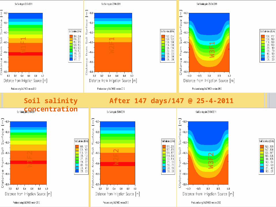
W2F1

W3F1

W1F1

Soil salinity concentration After 147 days/147 @ 25-4-2011

W1F2

W3F2

W2F2

Soil salinity content was lower in the 2nd growing season (Figure 159), compared to the 1st growing season (Figure 158).

لعمل الموديل يحتاجها التى Runالبياناتالتجربه إسم

الموقعالتجربة معامالت

الزراعة تاريخالحصاد تاريخ

 األرصاد ملف

الشمس : – – – سطوع ساعات عدد الرياح والصغرى العضمى الحرارة األرصاد بيانات - الشمسى اإلشعاع النسبيه الرطوبة

الرى ملفالرى + + + مياه ملوحة الرى إضافة ساعة ريه كل إضافة تاريخ ريه كل فى المياه كمية

المحصول ملفالفسيولوجية النمو مراحل تاريخ

فسيولوجيه - مرحله كل عند النبات فسيولوجيه LAIارتفاع مرحله كل عندالقش ومحصول الحبوب محصول

التربة  ملفاألمالح من طبقة كل ومحتوى طبقات الى وتقسيمها والكيمائي الميكانيكى التربه تحليل

والرطوبة والنتيروجينالذبول – – – – - نقطة الحقليه السعه الرطوبه من التربه محتوى المساميه C Eالقوام

إضافتها : التسميد   وميعاد والكمية السماد نوع

Thank you