Embed Size (px)
Citation preview

Critical evaluation of an automated
tool for heat exchanger network retrofits
based on pinch analysis and the Matrix
method Master’s Thesis within the Sustainable Energy Systems program
YANN LE STER & BERNHARD NOWICKI
Department of Energy and Environment
Division of Heat and Power Technology
CHALMERS UNIVERSITY OF TECHNOLOGY
Göteborg, Sweden 2013


MASTER’S THESIS
Critical evaluation of an automated
tool for heat exchanger network retrofits based on pinch
analysis and the Matrix method
Master’s Thesis within the Sustainable Energy Systems programme
YANN LE STER & BERNHARD NOWICKI
SUPERVISOR:
Elin Svensson
EXAMINER
Thore Berntsson
Department of Energy and Environment
Division of Heat and Power Technology
CHALMERS UNIVERSITY OF TECHNOLOGY
Göteborg, Sweden 2013
Critical evaluation of an automated tool for heat exchanger network retrofits based on
pinch analysis and the Matrix method
Master’s Thesis within the Sustainable Energy Systems programme
YANN LE STER & BERNHARD NOWICKI
© YANN LE STER & BERNHARD NOWICKI, 2013
Department of Energy and Environment
Division of Heat and Power Technology
Chalmers University of Technology
SE-412 96 Göteborg
Sweden
Telephone: + 46 (0)31-772 1000
Cover:
Example of matrix representation of a heat exchanger network in the program
Matrix.xla
Chalmers Reproservice
Göteborg, Sweden 2013

I
Critical evaluation of an automated tool for heat exchanger network retrofits based on
pinch analysis and the Matrix method
Master’s Thesis in the Sustainable Energy Systems programme
YANN LE STER & BERNHARD NOWICKI Department of Energy and Environment
Division of Heat and Power Technology
Chalmers University of Technology
ABSTRACT
The current climate change concern comes with new energy efficiency regulations. In
order to reach these new targets but also to get a more profitable process, plants have
to reconsider the design of their heat exchanger networks to reduce heat losses. One
way to proceed consists of retrofitting the network using the Matrix method in order
to get the cheapest solution achieving a defined level of heat savings. The software
Matrix.xla has been developed to run such a method. The main task of this thesis is to
analyze the accuracy of the results given by the method and the software. The
theoretical methodology behind the Matrix method is explained. The working
procedure of program Matrix.xla is enlightened and tested on specific examples to
point out several issues. Among these concerns, merging of the final solution,
introduction of split streams and handling utility streams are further investigated. A
complete solution is produced for the merging. However, given the complexity of the
splitting issue, only one specific solution is developed together with some highlights
of how to proceed for a general one. Concerning the utilities, a complete solution is
elaborated. Nevertheless, this solution can be pushed further by modifying some
concepts inside the Matrix method. Several ideas explaining how to proceed in this
direction are described. This work brings a better understanding of how a retrofit is
identified by the automated Matrix method tool and brings solutions to improve its
and the Matrix method’s routine. This is done in order to increase the applicability
and reliability of the Matrix method and the automated tool to identify better retrofit
solutions.
Key words:
Pinch analysis, Matrix method, Retrofit, Heat exchanger network, Stream splits.

II
Kritisk utvärdering av ett automatiserat verktyg för pinch analys med matrismetoden
Examensarbete inom masterprogrammet Sustainable Energy Systems
YANN LE STER & BERNHARD NOWICKI Institutionen för Energi och Miljö
Avdelningen för Värmeteknik och maskinlära
Chalmers tekniska högskola
SAMMANFATTNING
Den nuvarande problematiken med världens klimatändring har medfört nya
regleringar för en effektivisering av energiförbrukningen. För att kunna uppfylla dessa
nya krav men även få en lönsammare process, så har industrier övervägt sina
konstruktioner av värmeväxlarnätverk på nytt för att minska sina värmeförluster. Ett
tillvägagångssätt är att göra en retrofit av sitt nätverk genom att använda
matrismetoden för att få den billigaste lösningen för en fastställd nivå på sina
värmebesparingar. Programvaran Matrix.xla har utvecklats för att tillämpa denna
metod och huvudsyftet med denna avhandling är att analysera noggrannheten på
resultaten från denna programvara jämte metoden. Den teoretiska metodiken för
matrismetoden och programvaran förklaras. Arbetsgången för programvaran
Matrix.xla frambringas och provkörs på specifika exempel för att identifiera och peka
ut olika bekymmer med programvaran. Bland dessa problem görs en vidareutredning
utav en sammanfogning av den slutgiltiga lösningen, en introduktion av
strömdelningar samt metodens hantering utav externa uppvärmnings och
nedkylningsströmmar. En komplett lösning för sammanfogningen färdigställs. På
grund av tidsbristen och komplexiteten utav strömdelnings problemet dock, framställs
bara en specifik lösning för detta tillsammans med indikationer för en fortsatt
utveckling av en generell lösning. Angående uppvärmnings och
nedkylningsströmmarna så utarbetas en komplett fungerande lösning. Icke desto
mindre kan denna lösning utvecklas genom en modifiering av koncepten i
matrismetoden. Flera idéer som förklarar hur fortsättandet i den här riktningen bör ske
beskrivs. Det här arbetet ger en bättre förståelse för hur en retrofit identifieras utav
den automatiserade matrismetoden, samt ger lösningar för hur denna rutin ska
förbättras för att utöka tillämpligheten och tillförlitligheten av metoden och därtill
även identifiera bättre retrofit lösningar.
Nyckelord:
Pinchanalys, Matrismetoden, Retrofit, Värmeväxlarnätverk.

III
Contents
ABSTRACT I
SAMMANFATTNING II
CONTENTS III
PREFACE VII
NOTATIONS IX
1 INTRODUCTION 1
1.1 Background 1
1.2 Aim and objectives 2
1.3 Limitations 2
1.4 Thesis outline 2
2 METHODOLOGY 3
2.1 List of materials 3
2.2 Procedure 3
3 HEAT EXCHANGERS AND HEAT EXCHANGER NETWORKS 5
3.1 Description of heat exchangers 5
3.2 Heat Exchanger Networks 7
4 PINCH TECHNOLOGY 9
4.1 Description and history 9
4.2 Basic Concepts 9 4.2.1 Representation of a Heat exchanger network 9
4.2.2 Hot and Cold streams 10 4.2.3 Utilities 10
4.2.4 Pinch temperature 10 4.2.5 Pinch rules & violations 10
4.2.6 Composite Curves 11 4.2.7 Grand Composite Curves 12
4.3 Energy and cost targeting 12 4.3.1 Minimum Utility Demands targeting 12
4.3.2 Units targeting 13 4.3.3 Minimum Temperature Difference and Area targeting 13
4.4 Retrofitting heat exchanger networks 14
5 THE MATRIX METHOD 17
5.1 Introduction 17
5.2 What cost parameters are taken into account? 17

IV
5.3 What data is used from the current network? 17
5.4 What is the procedure? 18
5.4.1 Choice of global and pinch violations 18
5.4.2 The economic evaluation within the Matrix method 20
5.4.3 Hot and cold utilities 22
5.5 Summary of the method: 23
6 THE DIFFERENT CALCULATION TOOLS FOR THE MATRIX METHOD 25
6.1 Pro-Pi 25
6.2 Matrix.xla 26 6.2.1 The overall procedure of Matrix.xla 27 6.2.2 Manual choice of matches 31
6.3 Automated routine program 33 6.3.1 Matrix behavior 33
6.3.2 Optimization strategies 34 6.3.3 Flow chart 36
7 DESCRIPTION OF ISSUES IN THE MATRIX METHOD, THE
CALCULATION TOOL AND THE OPTIMIZER 37
7.1 Merging the solutions above and below the pinch 37
7.2 How to handle stream splitting 42
7.2.1 Definition + Example 42 7.2.2 Limitation 44
7.2.3 Possible improvement 47
7.3 How to choose the optimum ΔTmin 47
7.4 Improvement of the internal calculations (Costs) and better simplifications 47
7.5 Hot and cold utilities? 49
7.6 Other small issues 50
8 MERGING SOLUTION 53
8.1 Difference of cost between extension area and new heat exchanger 55
8.2 Methodology to generate the final merged solution 57
8.3 Diagram of the method 58
9 SOLUTION FOR STREAM SPLITTING 59
9.1 The two main situations requiring splitting 59
9.2 Using splitting instead of HEX’s requiring large areas 59
9.3 Identification of streams to split 60
9.4 Different splitting scenarios 61
9.4.1 Estimation of split ratio from current network: 61 9.4.2 Iterative method 66

V
10 IMPROVEMENT OF UTILITY CONSIDERATIONS IN THE MATRIX
METHOD 69
10.1 The issue 69
10.2 How to improve the method 76 10.2.1 Adding a utility cost at the end 76
10.2.2 Adding a saving cost to matches in different utility regions 76 10.2.3 Several solutions on a divided network 77
10.2.4 Including the utility streams inside the network as soft streams 78
11 CONCLUSION 79
12 SUGGESTIONS FOR FUTURE WORK 81
13 BIBLIOGRAPHY 83

VI

VII
Preface
In this study, tests have been performed with the software Matrix.xla and Pro-Pi
which both are Excel add-ins written in Visual Basic. The tests have been carried out
from January 2013 to June 2013. The work is a part of continuous improvement of
modelling tools at the Department of Energy and Environment, Division of Heat and
Power Technology, Chalmers University of Technology, Sweden.
This part of the project has been carried out with Doctor Elin Svensson as a supervisor
and Professor Thore Berntsson as examiner. All tests have been carried out at the
division of Heat and Power Technology at Chalmers University of Technology. The
cooperation with the PinexoTM
project has been very appreciated especially in the first
steps of the project to identify the issues at stakes. We would also like to thank Per-
Åke Franck at CIT Industriell Energi AB for his co-operation and involvement.
Finally, it should be noted that the tests could never have been conducted successfully
without the sense of high quality and professionalism of the laboratory staff and in
particular Elin Svensson.
Göteborg, June 2013
Yann Le Ster and Bernhard Nowicki.

VIII

IX
Notations
Roman upper case letters
A Area of a heat
exchanger, m2
Aadd Fixed investment cost
for adding area to an
existing HEX, m2
Afast Total area fixed heat
exchanger investment
cost of a match, m2
Afast1 Fixed investment cost
for new HEX or adding
area to an existing
HEX, m2
Afast2 Additional fixed
investment cost for a
specific match, m2
𝐴 Area of HEX in
solution given by the
MM above pinch, m2
Anew Fixed investment cost
for new heat exchanger,
m2
Ai Additional area, m2
𝐴 Initial area of a HEX
before retrofit), m2
Ai,saved Area of HEX i that has
been saved in
computer’s memory, m2
Amin Minimum area required
by the network, m2
Ce Electricity cost for
motor (pipe), $/kWh
Celi Electricity cost for
motor (inside), $/kWh
Celo Electricity cost for
motor (outside), $/kWh
C Power constant for
motor cost (pipe)
Ca Constant in heat
exchanger area cost
cArea Additional area cost, $
Ci Cold stream i
CiM Power constant in motor
cost (inside HEX)
CL Constant in pipe cost
CM Constant in motor cost
(pipe)
CMi Constant in motor cost
(inside heat exchanger)
CMo Constant in motor cost
(outside heat
exchanger)
Cp Specific heat, J/kg.K
Cp,c Specific heat cold
stream, J/kg.K
Cp,h Specific heat hot
stream, J/kg.K
CTot Area Total area cost, $
CW Cold Water
Dh Hydraulic diameter, m
Di Pipe intern diameter, m
Internal diameter of
HEX 1 tube, m
Do External diameter of a
concentric tube HEX, m
DT Temperature
difference,K
ΔT Temperature
difference,K
ΔTc Temperature difference
between inlet and outlet
of HEX for cold stream,
K

X
ΔTh Temperature difference
between inlet and outlet
of HEX for hot stream,
K
ΔTlm Log mean temperature
difference
ΔTmin Minimum temperature
difference, K
ΔTglobal Global temperature
difference, K
Global minimum
temperature difference,
K
ΔH Variation of enthalpy,
kJ/kg
F Mass flow, kg/s
Fc Mass flow cold stream,
kg/s
FCp Heat flow capacity,
kW/K
Heat flow capacity of a
stream going from
outside to the pinch,
kW/K
Heat flow capacity of a
stream going from the
pinch to outside, kW/K
Fh Mass flow hot stream,
kg/s
GCC Grand Composite Curve
HEN Heat Exchanger
Network
HEX Heat Exchanger
Hi Hot stream i
HP High Pressure
HEX Heat Exchanger
IES Industrial Energy
Systems
L Piping distance between
streams, m
LP Low Pressure
MER Maximum Energy
Recovery
MM Matrix Method
MP Medium Pressure
Ncold Number of cold streams
Nhot Number of hot streams
Nusselt number outside
HEX tube
Nusselt number inside
HEX tube
P Pressure, Pa
Pi Pressure (inside HEX),
Pa
Pifree Free available pressure
drop (inside), Pa
Po Pressure (outside HEX),
Pa
Pofree Free available pressure
drop (outside), Pa
Pr Prandtl number
Q Heat load, W
Qbef Real exchanged heat
load of HEX (based on
ΔTlm and UA), W
QC,min Minimum cold utility
demand, W
QH,min Minimum hot utility
demand, W
QHX Load of heat exchanger,
W
Qmax Maximum possible heat
load of a HEX, W
Qrest Remaining heat load on
a stream, W
Qsave Potential energy
savings, W
Qtot Total heat load of a
stream, W
Qutilities Utility demand, W

XI
Qwx Heat load of a HEX, W
rA Annuity factor for HEX
area, year-1
Reynold number
T Temperature, K
T cold in Temperature of the cold
stream entering heat
exchanger, K
Temperature of cold
stream entering heat
exchanger above pinch,
K
T cold out Temperature of cold
stream leaving heat
exchanger, K
Temperature of cold
stream leaving heat
exchanger below pinch,
K
T hot in Temperature of hot
stream entering heat
exchanger, K
Temperature of hot
stream entering heat
exchanger below pinch,
K
T hot out Temperature of hot
stream leaving heat
exchanger, K
Temperature of hot
stream leaving heat
exchanger pinch, K
Tpinch Pinch temperature, K
Tstart Starting temperature of
a stream, K
Ttarget Targeted final
temperature of a stream,
K
U Overall heat transfer
coefficient, W/m2.K
Umin Minimum amount of
units
VBA Visual Basic for
Applications
Roman lower case letters
b Power constant in heat
exchanger area cost or
in pipe cost
ca Constant in heat
exchanger area cost
cPiping Total piping cost, $
cpow Total electricity cost, $
cps Cost of motor (outside),
$
cpt Cost of motor (inside),
$
hi Convection heat
transfer coefficient
inside tube, W/m2.K
ho Convection heat
transfer coefficient
outside tube, W/m2.K
Mass flow, kg/s
Viscosity, kg/s.m
k Thermal conductivity,
W/m.K
x Splitting ratio, J/s.K

XII

1
1 Introduction
This introduction gives a brief overview of the thesis content, focusing on presenting
the subject background, purpose of the thesis, its goals and its limitations.
1.1 Background
Process industry heat exchanger networks are not always arranged in very energy
efficient set ups, therefore retrofit studies are recommended to be performed in order
to evaluate their possibly increased energy recoveries and cost savings. Pinch analysis
(Kemp 2007, Smith 2005), is an effective tool to evaluate the energy efficiency of a
network, and previous work based on pinch technology has led to different
approaches of performing retrofit studies. One of these approaches is the Matrix
method developed at Chalmers (Carlsson 1996), which this thesis is focused on. The
Matrix method results in an estimated overview for the trade-off between investment
costs and energy savings for retrofits. A program (Matrix.xla) has been developed as
an Excel add-in to facilitate the calculations of the method. This program is based on
another program named Pro-Pi (Franck 2010) for data input. There is also a capability
from within Matrix.xla to use an automated optimization routine (Matrix method
optimizer) to reduce the calculation times of performing all iterations required. Yet
the question of the reliability of the results is raised since some issues seem to remain,
such as; incapacity of the method and the program to adapt to some specific
situations, methodological and calculation errors, and the Matrix method optimizer
and its capacity to always reach the best solution. Many gaps have been identified, but
due to prioritized interest in other fields of science, little has been done to improve the
Matrix method and the program since 2001.
To sum up, there is the Matrix method which is the methodology to identify a close-
to-optimal retrofit of a heat exchanger network (HEN). The program Pro-Pi is used to
input stream data and data for the existing heat exchangers in the network. This data is
then used as an input by the Matrix calculation tool Matrix.xla that is a program
helping the user to perform the Matrix method calculations. Finally, an automatic
optimization routine referred to as the “Matrix method optimizer” is included as an
option inside the program Matrix.xla to enable the replacement of manual selections
by optimization.
In 2012, the PinexoTM
project was initiated to distribute retrofit software
commercially, and they are currently producing software based on the previously
mentioned Matrix method optimizer program. Due to this and scientific reasons, there
lies a large interest in evaluating the methods and assumptions behind the Matrix
Method and the previously written Matrix method optimizer program based upon it.

2
1.2 Aim and objectives
The objective of this master thesis is to critically investigate, evaluate and improve the
Matrix method, the Matrix calculation tool, and the automated routine for Matrix
method optimization. The goal is to produce a thesis open for public use, describing
and evaluating the strong points and drawbacks of the Matrix method and its
implementation in an automated tool, followed by suggestions and possible
improvements for the future. The main focus of the thesis is to do research on the
drawbacks and gaps of the method in order to develop and improve the reliability and
the working area of the Matrix method.
1.3 Limitations
One limitation to this work is that there has been no collection of stream data from an
actual process industry as this is much too time consuming (approximately 2 working
months for one person experienced in the field). All tests of the program have been
performed on previous scenarios created. Furthermore, since this is a master thesis
within the subject of Sustainable Energy Systems, it is not within the scope of the
subject to write code for the actual program itself. Proposed algorithms for method
improvements have been illustrated, and if found useful, they could later be translated
and implemented in code.
1.4 Thesis outline
The thesis starts with a theoretical section including a basic description of heat
exchangers followed by a brief overview of the basic concepts of pinch technology
and an explanation of the Matrix method (see Chapter 3, Chapter 4 and Chapter 5).
Then, the tools Pro-Pi, Matrix.xla and the automatic optimization routine are
described in Chapter 6. This first descriptive part of the thesis is then followed by
Chapter 7 which explains and illustrates the different issues identified in the Matrix
method and the tools. Chapters 8 to 10 show deeper analyses of the main issues
(merging, splitting and utilities) and bring solutions to these issues. Finally, results are
summed up and discussed in the conclusion (see Chapter 11). Given that every
separate issue has been handled in a different way the thesis does not include a
distinct general discussion part. The discussion section is integrated in every specific
chapter for every issue.
3
2 Methodology
The following chapter explains the methodology of how this thesis is carried out. The
procedures and the list of materials are presented.
2.1 List of materials
This thesis is mainly focused on evaluating a methodology and constructed programs
that carry this methodology out. Therefore a computer and software was enough for
carrying out this thesis. The software used in order to carry out this thesis work was
the following:
Excel
Pro-Pi (Franck 2010)
Matrix.xla (Franck and Berntsson 1999)
The Automatic optimization tool, MatrixOpt (Andersson 2001)
2.2 Procedure
The whole thesis was initiated by an analysis of the methodology behind the Matrix
method followed by a study of how to use the Pro-Pi and the Matrix.xla software
through several assignments and exercises in order to understand how they work but
also in order to identify their working area and their limitations.
After that, the Matrix method optimizer was analyzed and tested to see how it works
and applies the Matrix method. A list of all the data required for the programs by the
user was made. Subsequently the outcome that the user gets from the method was
detailed together with detailed descriptions of the program process paths followed.
These initial steps were followed by listing out the gaps and limitations of the
programs. The impacts of the limitations on the results were estimated and an
investigation of a selected set of the limitations found was initiated.
Each one of these in-depth studies of the selected set was done to understand and
describe them and examples were created to show the impact and consequences of
them on certain retrofit situations. This was followed by proposed solutions of how to
fix the gaps in order to make the method more efficient, more accurate and so as to
get a final solution with the best trade-off between investment costs and revenue from
energy savings.

4
5
3 Heat exchangers and heat exchanger networks
The following section presents a brief description about heat exchangers including
some general theory, different types and their modes of operation.
3.1 Description of heat exchangers
A heat exchanger (HEX) transports heat between streams going through the
exchanger. In a process industry this is a key component for heat recovery and lower
energy costs as it reduces the cooling demand of one stream at the same time as it
reduces the heating demand of another. Most HEX’s are designed to have counter
current flows or cross flows as this is a very efficient way to transfer heat, and all
HEX’s in this thesis and the Matrix calculation tool are assumed to mainly have these
modes of operation.
Any stream can only transfer heat to another stream if they have a temperature
difference according to the laws of thermodynamics, and the smaller the temperature
difference between these two streams is, the less the driving force for the heat transfer
between them will be. The heat load of a HEX (Q) is given by:
𝐴 (1.1)
where Q is the heat transfer rate [W], U is the overall heat transfer coefficient
[W/m2∙K], A is the heat transfer surface area [m
2], is the log mean temperature
difference [K] where ( )
( ) , and where are the temperature
differences between one stream’s inlet and the other stream’s outlet.
For a detailed explanation about the heat transfer driving forces and heat transfer
properties, see Incropera et al. (2007).
Since the heat load (Q) depends on the temperature difference between the two
streams, HEX’s that operate between small temperature differences need to be
efficient by heat exchanging through a large heat exchanging surface area, which is
quite costly. The larger the heat exchanging surface area in a HEX is, the more heat
can be transferred.
One of the simplest types of HEX’s is the counter flow concentric tube type heat
exchanger, see Figure 3.1. This HEX has one fluid flowing inside a tube in one
direction and another external fluid flowing outside of the tube in the opposite
direction along the annular gap between the inner tube and an external tube. The
fluids exchange heat throughout this process as one fluid is hotter than the other. This
HEX is used for simplicity when calculating an optimal solution for stream splitting in
this thesis in Chapter 9.

6
Figure 3.1 A counter flow concentric tube type heat exchanger with one fluid
flowing through the inner tube in one direction and the other fluid flowing through the
annular gap in the opposite direction.
An example of a more commonly used HEX that transfers heat between liquids is a
shell and tube type of heat exchanger, see Figure 3.2. This HEX adds the effect of
cross flow and turbulent flow which is often more efficient than simple flow along the
length of a tube.
Figure 3.2 The liquid coming in at the tube inlet passes through the tubes and
comes out at the tube outlet. The second liquid entering at the shell inlet passes
through in between the tubes and works its way through the course set up by the
baffles until it finally exists at the shell outlet. The liquids exchange heat throughout
this process in a cross-counter flow without being mixed.
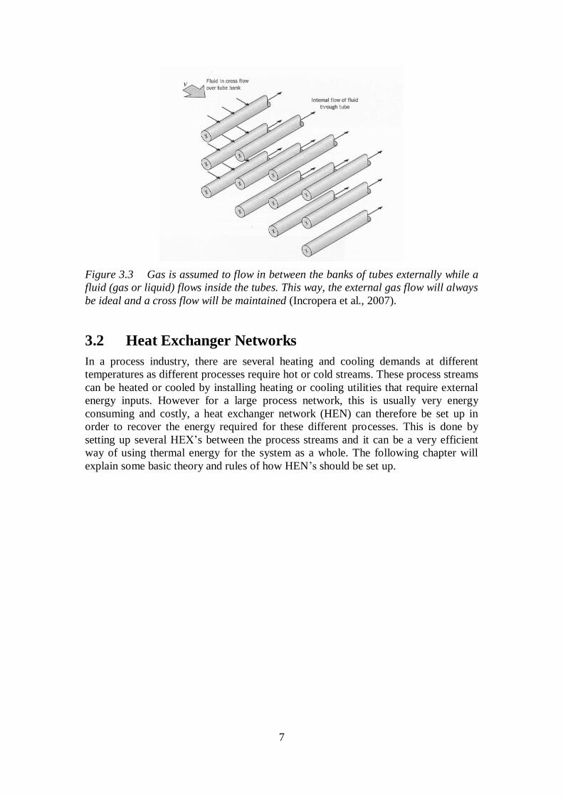
All calculations of heat exchange between liquids performed by the Matrix calculation
tool are based on shell and tube type heat exchangers. When it comes to gas streams,
heat exchange across ideal tube banks (cross flow heat exchanger) are assumed which
looks like the following (see Figure 3.3):
7
Figure 3.3 Gas is assumed to flow in between the banks of tubes externally while a
fluid (gas or liquid) flows inside the tubes. This way, the external gas flow will always
be ideal and a cross flow will be maintained (Incropera et al., 2007).
3.2 Heat Exchanger Networks
In a process industry, there are several heating and cooling demands at different
temperatures as different processes require hot or cold streams. These process streams
can be heated or cooled by installing heating or cooling utilities that require external
energy inputs. However for a large process network, this is usually very energy
consuming and costly, a heat exchanger network (HEN) can therefore be set up in
order to recover the energy required for these different processes. This is done by
setting up several HEX’s between the process streams and it can be a very efficient
way of using thermal energy for the system as a whole. The following chapter will
explain some basic theory and rules of how HEN’s should be set up.

8

9
4 Pinch Technology
The Matrix method, which is the main methodology used by Matrix.xla and
PinexoTM
’s software is based on Pinch technology, and this section of the thesis will
briefly explain its most relevant concepts, methods and outcomes.
4.1 Description and history
Pinch technology provides the main analytical methodology, also called Pinch
analysis, which is utilized by the Matrix method. The identification of the heat
recovery pinch in 1982 and 1978 by Linnhoff (1982) and Umeda (1978)
independently, lead to the spark that ignited Pinch technology that was developed
throughout the remaining decades of the 20th
century. Pinch technology provides a
methodology that analyses energy flows of complex industrial processes in order to
save energy. By stepwise following this methodology, the HEN solution with the
fewest number of units that are required to reach the minimum energy consumption
can be identified, that is; a Maximum Energy Recovery (MER) network.
For more details, the interested reader is referred to one of the standard textbooks
about pinch analysis by Kemp (2007) or Smith (2005).
4.2 Basic Concepts
4.2.1 Representation of a Heat exchanger network
A HEN can easily be represented as in the following Figure 4.1.
Figure 4.1 Example of representation of a HEN including a cold stream, a hot
stream, a cooler, a heater and a heat exchanger.
This is how the HEN’s are represented throughout this thesis as well as in Pro-Pi. T
represents temperature in 0C, H represents an external heater, C represents an external
cooler, the duty is the heat power of the utility/HEX and is normally represented in
kilo-Watts, FCp is the mass flow multiplied with the with the specific heat of the
medium.
10
4.2.2 Hot and Cold streams
In a HEN, a hot stream is defined as a material stream that has a specified flow and
heat capacity with a cooling requirement in order to change its temperature from a
supply to a target value. A cold stream is defined as a material stream that has a
specified flow and heat capacity with a heating requirement in order to change its
temperature from a supply to a target value. Thus a hot stream implies a cooling
demand while a cold stream implies a heating demand. If a hot or a cold stream has
been heated up or cooled down according to the size of its heating or cooling demand,
it can be regarded as being “ticked off” in the network. Streams can also have soft
target temperatures, this implies that their target temperatures necessarily do not have
to be reached, however the streams may still be used in order to heat or cool other
streams in the HEN.
In most of this thesis and in Pro-Pi, illustrated hot streams are represented with red
color and illustrated cold streams are represented with blue color.
4.2.3 Utilities
Utilities are the heating and cooling media used in heaters and coolers. A hot utility in
a HEN is a utility such as steam that heats a cold process stream while a cold utility,
for example cooling water, cools a hot process stream.
4.2.4 Pinch temperature
The heart of pinch technology is the identification of the so-called pinch temperature
in a HEN. The pinch temperature, or pinch as it is commonly called can be identified
graphically or mathematically. In order to identify the pinch temperature graphically,
composite curves for all the streams in the network are constructed (see Section
4.2.6). The hot composite curve and the cold composite curve are then drawn on a
(ΔH, T) diagram and matched together in order to give the most energy recoverable
solution by matching them as closely together as possible without violating the
minimum temperature difference (ΔTmin) established for the HEN. The point where
the ΔTmin between the hot and the cold streams occurs is called the pinch. Looking at
Figure 4.2 on the next page; it looks like the curves are being pinched together at this
exact temperature difference, hence the word pinch is commonly notated for this
interval.
4.2.5 Pinch rules & violations
One of the most important concepts in Pinch technology is the one concerning the
three golden pinch rules and their violations.
Heat should not be transferred in the system through the pinch
External heating should not be done to the system below the pinch
External cooling should not be done to the system above the pinch
If these rules are violated, it will not be possible to obtain a MER network. This is
because if external heat is added below the pinch, the same amount needs to be cooled
externally. If heat is subtracted externally above the pinch, the same amount has to be

11
added externally. If heat is transferred through the pinch, it needs to be added and
subtracted later to the system. In a network the sum of the pinch violations are the
potential energy savings, that is, the difference between the present and the minimum
utility demand. HEN’s are therefore often represented as two separate ones, one above
and one below the pinch in order to not violate any of these rules accidently.
4.2.6 Composite Curves
Composite curves can be defined as theoretical compositional streams for the existing
hot and cold streams of a network system. They are constructed by calculating the
total enthalpy contents of all the existing streams through certain temperature intervals
for the hot and the cold streams separately. An example of what they look like is
shown in Figure 4.2.
Figure 4.2 Composites curves for hot and cold streams, minimum heating demand,
minimum cooling demand and location of the pinch.
Constructing heat cascade diagrams and using an algebraic algorithm as suggested
and described by Kemp (2007) is the other way to identify the pinch. The pinch is
easily identified mathematically with help from computational methods based on such
cascade calculations implemented in software such as Pro-Pi (Franck 2010) and this is
how it’s done throughout this thesis work.
Once the pinch temperature has been identified, the network is divided into two parts.
One part above the pinch where there is a heat deficit, a need for heating that is, and
one part below the pinch and here there is a heat surplus, which means that there is a
need for cooling. QHX in Figure 4.2 is the amount of heat that can be recovered (heat
exchanged) between the streams in the network.

12
4.2.7 Grand Composite Curves
A great way to illustrate energy flows of a HEN is through a Grand Composite Curve
(GCC), also called a heat surplus diagram, see Figure 4.3. It represents the net surplus
and deficit of enthalpy of the network for different temperature intervals both above
and below the pinch, and through a GCC the minimum heating and cooling utilities,
the division of the network above and below the pinch temperature and the heat flow
direction between the temperature intervals can be identified. A GCC is one of the
results illustrated by Pro-Pi whenever stream data is entered. Important to notice is
that all the hot and cold “net deficit streams” have been subtracted and added by
ΔTmin/2 respectively.
Figure 4.3 Example of a Grand Composite Curve for a HEN (Harvey 2011)
4.3 Energy and cost targeting
4.3.1 Minimum Utility Demands targeting
In a pinched HEN, there is always a minimum heating and cooling utility demand for
the streams. These minimum utility demands are identified through the pinch division
of the network after setting up a global ΔTmin for which the HEX’s may operate. The
minimum heat utility demand (QH,min) can be defined as the minimum amount of
external heating that is needed in a HEN while the minimum cooling utility demand
(QC,min) can be defined as the minimum amount of external cooling that is necessary
for a HEN, they are both illustrated in Figure 4.2 and 4.3. Since energy is costly, the
target is usually set for as low of an external utility demand as possible, and by
subtracting the present heating and cooling network demands with QH,min and QC,min
respectively, the potential energy savings (Qsave) are calculated.
13
4.3.2 Units targeting
Any unit described in this thesis is one that does a change to the heat energy
(enthalpy) of a stream through a HEX. It can be done by heat exchanging the streams
with each other in a HEX or by utilizing a utility media in a heater or cooler. In the
grass root design of a network, the target is usually set for as few units as possible as
this often is less costly. According to Euler’s network theorem (Kemp 2007), the
minimum amount of units (Umin) that are required to achieve a HEN with a heat
recovery to a certain degree can be determined. This estimation can be used in order
to analyze designs of HEN’s for setting a target for the amount of units, and still
achieve a desirable heat recovery.
Important to notice is that for retrofit situations, the amount of existing units probably
already exceeds Umin. It is therefore usually not preferable to aim for the minimum
number of units in a retrofitted network. What is important is instead to minimize the
number of new units.
4.3.3 Minimum Temperature Difference and Area targeting
As explained in the previous chapter, the temperature difference and heat transferring
area between two streams in a HEX influences the amount of heat that can be
transferred between them. However, it is rather costly to dimension HEX’s to operate
with small temperature differences as this requires a large HEX area. The larger the
HEX area is, the more efficient, yet more expensive the HEX will be. A smallest
allowable temperature difference ΔTmin between any two streams in a HEN is
therefore chosen due to economic and thermodynamic considerations.
The ΔTmin chosen for a network influences the amount of energy that can be
recovered because with a smaller ΔTmin allowance for a network, more energy may be
exchanged between each set of one hot and cold stream in a HEX. A ΔTmin can either
be set globally for all the streams or set individually for the streams analyzed. In grass
root design, the optimal and most economic global ΔTmin for a HEN is retrieved by
considering costs for energy consumption against investment cost targets for a chosen
set of different ΔTmin. This includes costs for the minimum amount of units, heat
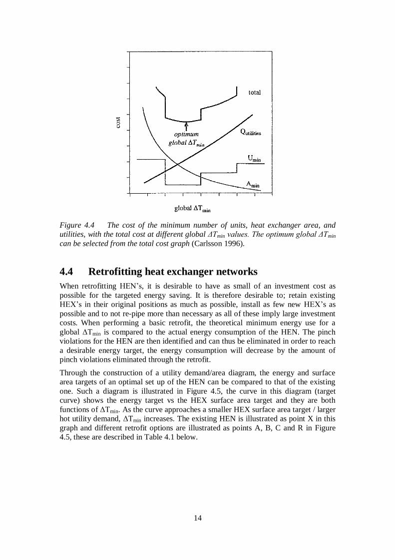
exchanger area, and the energy costs, see Figure 4.4. When it comes to a network
retrofit situation, finding an optimum global ΔTmin is more difficult and therefore less
reliable. In the retrofit case, the existing HEX area must be considered, for example,
as suggested by Tjoe (1984), by comparing it to the minimum HEX area required for
the current heat recovery level and based on that a global ΔTmin can be selected.
14
Figure 4.4 The cost of the minimum number of units, heat exchanger area, and
utilities, with the total cost at different global ΔTmin values. The optimum global ΔTmin
can be selected from the total cost graph (Carlsson 1996).
4.4 Retrofitting heat exchanger networks
When retrofitting HEN’s, it is desirable to have as small of an investment cost as
possible for the targeted energy saving. It is therefore desirable to; retain existing
HEX’s in their original positions as much as possible, install as few new HEX’s as
possible and to not re-pipe more than necessary as all of these imply large investment
costs. When performing a basic retrofit, the theoretical minimum energy use for a
global ΔTmin is compared to the actual energy consumption of the HEN. The pinch
violations for the HEN are then identified and can thus be eliminated in order to reach
a desirable energy target, the energy consumption will decrease by the amount of
pinch violations eliminated through the retrofit.
Through the construction of a utility demand/area diagram, the energy and surface
area targets of an optimal set up of the HEN can be compared to that of the existing
one. Such a diagram is illustrated in Figure 4.5, the curve in this diagram (target
curve) shows the energy target vs the HEX surface area target and they are both
functions of ΔTmin. As the curve approaches a smaller HEX surface area target / larger
hot utility demand, ΔTmin increases. The existing HEN is illustrated as point X in this
graph and different retrofit options are illustrated as points A, B, C and R in Figure
4.5, these are described in Table 4.1 below.

15
Figure 4.5 HEX surface area vs hot utility demand curve
HX
Surf
ace
Are
a
Hot Utility Demand
X
R
C
B
A
Existing networkCriss-cross HX
Target curveVertical HX:ing
Different values of ΔTmin

16
Table 4.1 Description of different situations from Figure 4.5
Retrofit Approach Result & Evaluation
X → A
The HEX surface area is reduced to its
minimum necessary value without
decreasing the hot utility demand. This
option does not make use of the existing
HEX surface area and is therefore a poor
retrofit option.
X → B
The HEX surface area is reduced to that
of an optimum grass root design at the
same time as the hot utility demand is
decreased. The entire installed HEX
surface area is not utilized and thus this is
not optimal for a retrofit.
X → C
The entire HEX surface area installed is
utilized and used in its best way after the
retrofit. The hot utility demand is
decreased to its minimum for the area
available. This is a very good retrofit
option but in practice not possible as
HEX’s already are optimized for certain
conditions.
X → R
This is a great retrofit option close to that
of C, however more realistic since new
HEX area usually needs to be installed.
The area installed is used to its best
capacity and as little new area as possible
is installed. The heating demand is
reduced significantly.

17
5 The Matrix method
5.1 Introduction
The Matrix method (Carlsson 1996) has been developed to bring economically
optimal solutions to retrofit situations. Indeed, retrofitting HEN’s cannot be handled
by the traditional pinch design method. A retrofitting situation requires a
consideration of the limitations of the current network and using the traditional pinch
method would lead to dead end solutions because it would lead to a MER network
that is not economically affordable. The Matrix method aims at determining the
optimal amount of energy savings to pursue by taking the characteristics of the
existing network into account. Several of these parameters such as the distance
between the different streams are not thermodynamic data but they influence the cost
of the retrofitted solution directly. The Matrix method is a procedure helping the user
identifying the HEX’s that are wasting energy, and it aids the user to decide how to
modify the network in the cheapest way, by promoting the use of free already existing
HEX’s for example. It will not provide a single optimal situation but will result in
several cost-effective solutions for different energy recovery levels.
5.2 What cost parameters are taken into account?
The Matrix method aims at including all the costs of the retrofitting work and to
evaluate how they impact the final solution. The main parameters considered for cost
calculations are the following (Carlsson 1996):
The heat exchanger area
The type of heat exchanger
The construction material
The piping costs (distance between streams, pipes diameters, construction
materials)
The Pressure drop costs (pumps and pumping power costs)
Auxiliary equipment (valves)
Space requirements
Maintenance costs (cleaning, fouling)
5.3 What data is used from the current network?
In addition to all the previous cost data, the Matrix method also requires information
about the current network such as stream data (flow rate, heat capacity, supply and
target temperatures, density, viscosity, thermal conductivity, fouling factor) and HEX
data (UA-values, location, type, hydraulic diameter of both sides of the HEX).

18
5.4 What is the procedure?
5.4.1 Choice of global and pinch violations
The first step of a retrofit analysis is to choose a global ΔTmin for the retrofitted
network. This new ΔTmin has to be smaller than the one used in the current network.
Then, pinch analysis is used to calculate , and plus to identify the
HEX’s that violate the pinch rules. Several ΔTmin’s should be investigated by the user.
After that, the user has to choose which pinch violations that should be removed. The
more violations that will be removed, the more energy savings there will be, but that
also requires having a larger investment in new HEX’s and HEX modifications. At
this point the user has to select an optimum number of new and rearranged units. To
do so, a table pointing out the size of the violations for every HEX at various global
ΔTmin has to be built, see Table 5.1.
Table 5.1 Example of table representing the different violations for every heat
exchanger of the network at different values of global ΔTmin.
Heat exchangers of the current network
ΔTmin HEX1 HEX2 HEX3 HEX4 HEX5 HEX6 HEX7
ΔT1 - - V4 - V10 - V11
ΔT2 - - V5 - V10 - V12
ΔT3 - V2 V6 - V10 - V13
ΔT4 - V2 V7 V9 V10 - -
ΔT5 V1 V3 V8 V9 V10 - -
In this table no values are used, instead 13 hypothetical different levels of violations
are symbolized as V1 to V13.
Since HEX’s transferring heat from below to above the pinch point do not increase
the energy consumption, they should not be modified. Instead, only HEX’s
transferring energy in the opposite direction (heat from above to below the pinch
temperature) have to be investigated. Moreover, for each global ΔTmin investigated,
the user might first choose to eliminate only the biggest violations and allow the small
ones. Such a choice requires a splitting of the study of the network into two parts
(above and below the pinch) so that the internal HEX’s that are allowed to violate the
pinch rules can remain in their current positions.
Then, the economic part of the Matrix method is pursued (described in detail below)
to evaluate the cost of the different retrofit opportunities deleting the largest
violations. This procedure has to be run several times, with different values of global
ΔTmin’s and by rearranging different violations resulting in Figure 5.1 and Figure 5.2.

19
Figure 5.1 Development of retrofitting costs for different levels of energy recovery
Figure 5.2 Development of retrofitting costs for different levels of energy recovery
and different values of global ΔTmin.
At this point, the user can choose which global ΔTmin and which violations that have
to be fixed in order to get the cost per unit of saved energy ratio that suits him/her the
best.
0
1
2
3
4
5
6
7
9
8
0 10 12 14 168642
Q [MW]save
Co
st [
M$]
global T = 4 C mino
global T = 7 C mino
global T = 10 C mino
global T = 13 C mino
global T = 16 C mino

20
5.4.2 The economic evaluation within the Matrix method
When the user has chosen a global ΔTmin and decided what violations to eliminate for
the HEN, the reduction of the energy consumption is fixed. If some violations are
authorized to remain in the retrofitted network, the minimum utility consumption
(QH,min) will not be reached. In fact, the hot utility savings will only be as high as the
sum of the violations deleted. At this point, the process streams are separated into two
parts at the pinch temperature. In order to allow the authorized pinch violating HEX’s
to remain at their positions (temperature), the streams are not strictly separated at the
pinch point, see Table 5.2.
For example, in this network from a course compendium (Harvey 2011), the network
represented in Figure 5.3 has a pinch temperature of 114°C and a ΔTmin value of 22 K.
Figure 5.3 Network used as an example for economic evaluation within the Matrix
method.
The user can decide to retain the match H2-C2 even if it constitutes a pinch violation
of heat transfer through the pinch. In that case after dividing the system into two parts,
the user can choose to represent the streams above the pinch as following.
Table 5.2 Representation of streams above pinch including stream C2, violating the
pinch.
Stream Tstart Ttarget Q [kW]
H1 175 125 500
H2 125 98 1080
C1 103 155 1040
C2 40 112 1080
We can observe that H1 and C1 are limited by the pinch temperature while C2 is going
through it. This is how the division of the network has to be done, taking the
untouched HEX’s into account. The analysis of the retrofit is then done by
constructing a matrix for the two separated systems. Rows correspond to hot streams
and columns to cold ones. After this step, different kinds of matches are investigated
between all the different streams. Several matching situations are possible. In the first
situation, the heat load of a match is determined when the cold stream or the hot
stream is ticked off. The second possible situation is when we use the maximum heat
exchanging capacity of a currently existing HEX.
Qtot FCp
H1 45 175 1300 10V1
H2 65 C 98 125 2400 40C4 V3
C1 20 85 H 155 2700 20V1 H2
C2 40 112 1080 15V3

21
Finally, in some situations a match cannot be found between two streams by ticking one
off. In such a case, the match is pursued until a specified temperature difference is
reached between the streams. This ΔT has to be set as an input by the user. More
precisely, the different types of matches in the Matrix method are the ones in Table 5.3:
Table 5.3 The different types of matches in the Matrix method.
Cold Tick-Off The cold stream reaches its target temperature and is not possible
to use in any following match.
Hot Tick-Off The hot stream reaches its target temperature and is not possible to
use in any following match.
No Tick-Off None of the streams is fully used.
Not Possible The match is not thermodynamically possible.
Heater Hot utility is used for heating a stream.
Cooler Cold utility is used for cooling a stream.
Above the pinch a hot tick-off can be divided into three cases:
1. The cold stream can be used in a direct following match to tick-off another hot
stream.
2. The cold stream will be ticked off if it is used immediately in the next match.
3. It is not possible to use the cold stream in the next match.
If “cold” and “hot” changes place in the list above, the situation for a cold tick-off
below pinch is also explained.
The first matrix starts at the pinch point. The user has to investigate every possible (or
not possible) match between all the different streams. The user has to calculate the
optimum design and cost match for every couple of streams and write the cost of the
chosen match in the corresponding cell of the matrix. To do so, the user has to follow
an optimum routine in selecting matches. The routine described by Franck and
Berntsson (1999) in the paper “The Matrix method – the program Matrix.xla” is one
possible procedure to choose a match between two streams above the pinch.

22
Select matches in the following order:
Select hot streams that can be matched in only one way.
Select hot streams that have no existing HEX. Select matches in order of cost
but avoid ticking-off the cold stream if an existing HEX is located on the cold
stream.
Select existing matches.
Select matches in order of cost. The match with the lowest cost should be
selected first. If the most economical match hinders the possibilities of
deriving a solution at the stipulated heat recovery level, this match should not
be selected. This information is gained from the type of the match. If two
matches of equal economic merit exist, priority is given to match type 1 over 2
and 2 over 3.
The procedure is the same below the pinch if we replace “hot” by “cold”.
Every time a match is selected, a new matrix without the ticked-off stream (if it is
ticked-off) has to be calculated in order to implement the consequences of the
selection of this match on the remaining streams to match. The user has to proceed
like this until all the relevant streams are ticked-off and the desired energy recovery is
reached (the targeted violations are eliminated). At this point, the total cost of the
retrofit for the specific energy recovery can be calculated.
The user can then proceed to a new investigation of another way to match the streams
(if some matches were not obvious) and compare the new total cost of the retrofit to
make his/her final choice.
Finally, the user can do a new iteration of this method with a different targeted energy
recovery (by deleting more violations for example) and appreciate if the ratio of the
energy saved/cost is better than the previous solution.
5.4.3 Hot and cold utilities
Hot and cold utility HEX’s (heaters and coolers) are included in the matrix in the
same way that internal HEX’s are. However, hot and cold utilities cannot be ticked-
off since they aim at ticking off the internal hot and cold streams. Therefore, they are
used after all the streams are used for internal heat exchange to reach the temperature
goals of the un-ticked-off streams remaining. The aim is to reduce the heat load of the
utility streams. The size and price of the coolers/heaters are calculated when only
colds streams remain above the pinch and only hot streams below the pinch. Their
costs are included in the total cost for the retrofitted solution given by the Matrix
method.

23
5.5 Summary of the method:
Figure 5.4 Diagram summing up the overall Matrix method
Step2: Select one ΔTmin for deeper investigation
Step1: Create a table with the quantified pinch violations corresponding to various
global ΔTmin’s
Step3: Decide what violations have to be deleted, get a target for energy recovery
and divide the network into two parts at the pinch according to untouched HEX’s
Step4: Calculate the optimum design and cost of all the remaining matches (start at
the pinch) and complete the matrix with it
Step5: Select matches according to the routine explained before
Step6: Are all relevant streams ticked-off and is the targeted energy recovery reached?
Step7: Calculate the overall cost of the retrofitted solution for this specific energy
recovery
Step8: Have you investigated enough different energy recovery targets at this global
ΔTmin?
Step10: Have you investigated enough retrofit solution at different global ΔTmin values?
Step9: Compare and select the most economical energy recovery at this global ΔTmin
Step11: Compare and select the most interesting combinations for the energy
recovery, ΔTmin and the retrofited solution associated to them. Plotting Costs vs
Energy savings for several global ΔTmin can be
helpful here

24

25
6 The different calculation tools for the Matrix
method
This chapter describes the main inputs and outputs of the program Pro-Pi that
produces the stream data required to run the Matrix method. The main steps followed
in the software Matrix.xla are also described, including the logic behind the automatic
optimization routine (Matrix method optimizer).
6.1 Pro-Pi
Pro-Pi is an Excel add-in tool developed by CIT Industriell Energi AB to help its user
to do energy analysis of HEN’s using pinch analysis.
The program requires several inputs from the user in order to describe the network
such as:
Stream temperatures
Stream mass flows
Stream specific heats
ΔTmin for each stream or the global ΔTmin
Heat transfer coefficients
Utility data
From this data, Pro-Pi is able to draw a stream representation of the network (see
Figure 6.1), generate GCC’s (see Figure 6.2), retrieve HEX data (previously manually
placed by the user), evaluate pinch violations in the network (see Figure 6.3) and
enable the user to try different modifications of the network (changing HEX’s, heaters
and coolers). Pro-Pi is not “automated”, even if it does some calculations on its own
such as output temperatures, input temperatures, heat loads and violations, it is the
user that has to design the network by placing the different HEX’s manually.
Figure 6.1 Example of representation of a heat exchanger network in Pro-Pi
26
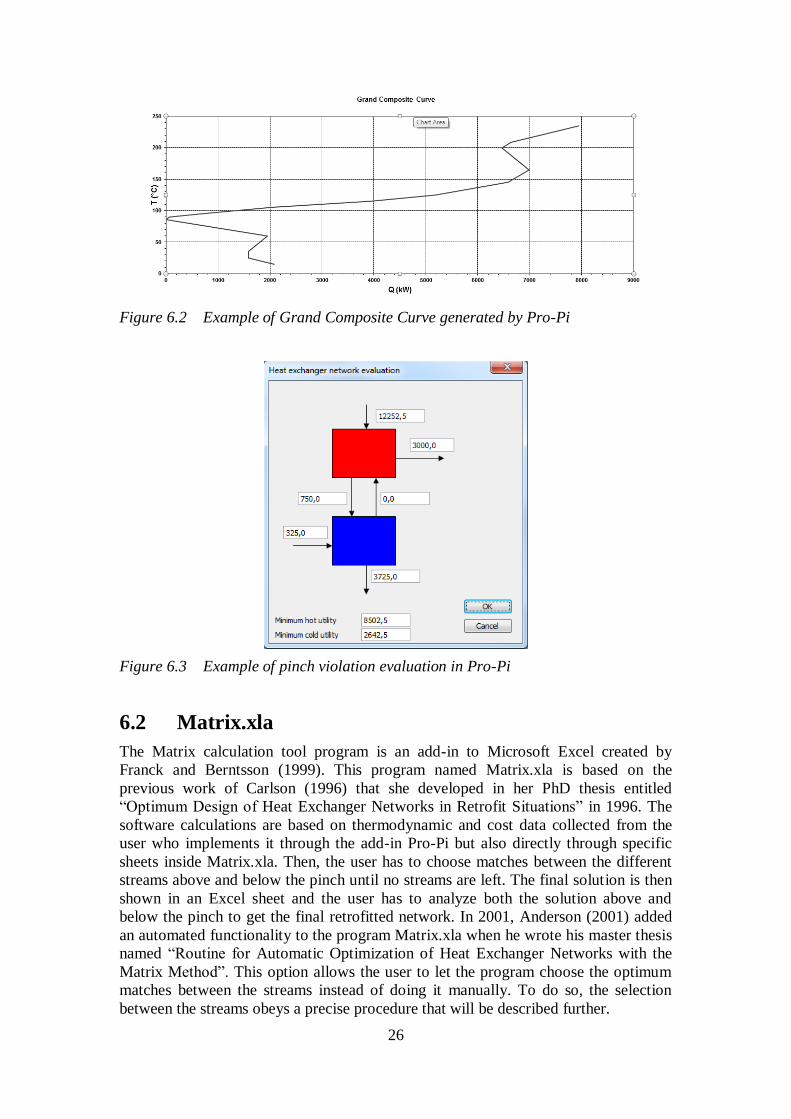
Figure 6.2 Example of Grand Composite Curve generated by Pro-Pi
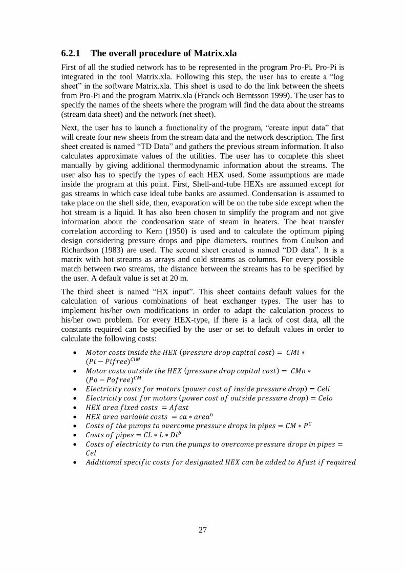
Figure 6.3 Example of pinch violation evaluation in Pro-Pi
6.2 Matrix.xla
The Matrix calculation tool program is an add-in to Microsoft Excel created by
Franck and Berntsson (1999). This program named Matrix.xla is based on the
previous work of Carlson (1996) that she developed in her PhD thesis entitled
“Optimum Design of Heat Exchanger Networks in Retrofit Situations” in 1996. The
software calculations are based on thermodynamic and cost data collected from the
user who implements it through the add-in Pro-Pi but also directly through specific
sheets inside Matrix.xla. Then, the user has to choose matches between the different
streams above and below the pinch until no streams are left. The final solution is then
shown in an Excel sheet and the user has to analyze both the solution above and
below the pinch to get the final retrofitted network. In 2001, Anderson (2001) added
an automated functionality to the program Matrix.xla when he wrote his master thesis
named “Routine for Automatic Optimization of Heat Exchanger Networks with the
Matrix Method”. This option allows the user to let the program choose the optimum
matches between the streams instead of doing it manually. To do so, the selection
between the streams obeys a precise procedure that will be described further.
27
6.2.1 The overall procedure of Matrix.xla
First of all the studied network has to be represented in the program Pro-Pi. Pro-Pi is
integrated in the tool Matrix.xla. Following this step, the user has to create a “log
sheet” in the software Matrix.xla. This sheet is used to do the link between the sheets
from Pro-Pi and the program Matrix.xla (Franck och Berntsson 1999). The user has to
specify the names of the sheets where the program will find the data about the streams
(stream data sheet) and the network (net sheet).
Next, the user has to launch a functionality of the program, “create input data” that
will create four new sheets from the stream data and the network description. The first
sheet created is named “TD Data” and gathers the previous stream information. It also
calculates approximate values of the utilities. The user has to complete this sheet
manually by giving additional thermodynamic information about the streams. The
user also has to specify the types of each HEX used. Some assumptions are made
inside the program at this point. First, Shell-and-tube HEXs are assumed except for
gas streams in which case ideal tube banks are assumed. Condensation is assumed to
take place on the shell side, then, evaporation will be on the tube side except when the
hot stream is a liquid. It has also been chosen to simplify the program and not give
information about the condensation state of steam in heaters. The heat transfer
correlation according to Kern (1950) is used and to calculate the optimum piping
design considering pressure drops and pipe diameters, routines from Coulson and
Richardson (1983) are used. The second sheet created is named “DD data”. It is a
matrix with hot streams as arrays and cold streams as columns. For every possible
match between two streams, the distance between the streams has to be specified by
the user. A default value is set at 20 m.
The third sheet is named “HX input”. This sheet contains default values for the
calculation of various combinations of heat exchanger types. The user has to
implement his/her own modifications in order to adapt the calculation process to
his/her own problem. For every HEX-type, if there is a lack of cost data, all the
constants required can be specified by the user or set to default values in order to
calculate the following costs:
( ) ( )
( ) ( )
( ) ( ) 𝐴
𝐴 𝐴

28
The user can change the values of all the constants present in the formulas above
(except for the physical data such as pressures and areas that are calculated) in the
sheet “HX input”. By summing all these costs for every HEX, the program estimates
the overall cost of the retrofitted network. The last sheet generated is the “UA data
sheet”. It is a matrix with hot streams in rows and cold ones in columns. The program
calculates the UA-values of the existing HEX’s in this matrix. If more than one HEX
is used between the two same streams, their UA values are added.
The next step in using the program consists of selecting a few global ΔTmin values to
carry out the analysis with. This temperature difference does not refer to the
temperature difference inside the HEX’s but it’s used to specify different energy
saving levels to investigate. The choice of this value should results from a previous
study of minimum utility versus that is not available in the Matrix.xla
program, but can be handled in Pro-Pi.
At this point, a first value of is investigated. Pro-Pi is used to draw a list of
the existing HEX’s and show which ones violate the pinch rules, and by how much.
At this point, the user has to choose which units to rearrange in order to reach a
certain energy saving (see Table 6.1). The user also has to refer to this sheet in the log
sheet for the program to be able to get access to this information.
Table 6.1 Example of a sheet used for the selection of violations to be retrofitted in
Matrix.xla
It is now required to divide the stream data into two parts at the selected . In
order to avoid costly heat exchanging at very small temperature differences the user is
invited to specify a minimum temperature difference in HEX’s where tick-off is
thermodynamically possible and also one for those where tick-off is not
thermodynamically possible. The division of the network into two parts generates two
new sheets. These sheets represent the name, type, starting temperature, targeted
temperature and heat load of the streams above and below the pinch. It also takes the
accepted pinch violations into account by representing these HEX’s both in the
regions above and below the pinch. Consequently these violating HEX’s have to be
matched in both regions (see Table 6.2 and Table 6.3).

29
Table 6.2 Example of representation of the streams above the pinch after network
splitting at the pinch in Matrix.xla. The violation on HEX #2 is rearranged.
Table 6.3 Example of representation of the streams below the pinch after network
splitting at the pinch in Matrix.xla. The violation on HEX #2 is rearranged.
For example, HEX #2 connecting stream number 2 and 5 shows a violation of
360 kW through the pinch. Since this violation has been asked to be rearranged (see
Table 6.1), stream 2 is strictly divided at the pinch in AP data and BP data (From
94.5°C to 90.5°C above and then, from 90.5°C to 64.5°C below). If we run the
division of the network again without asking for this violation to be rearranged, we
get the following tables (see Table 6.4 and Table 6.5):
Table 6.4 Example of representation of the streams above the pinch after network
splitting at the pinch in Matrix.xla. The violation on HEX 2 is not rearranged.

30
Table 6.5 Example of representation of the streams below the pinch after network
splitting at the pinch in Matrix.xla. The violation on HEX 2 is not rearranged.
In this case, stream 2 is not stopping at Tpinch anymore but goes straight down to
64.50C even in AP data. This section of the stream is then represented both in AP data
and BP data. That difference clearly points out that the network division deals with
authorized violations and that these HEX’s will be matched both above and below the
pinch which has to be considered by the user when he will have to build the overall
retrofitted solution, gathering above and below pinch solutions. Moreover if the
Matrix method optimizer suggests adding a new HEX for a stream that is represented
in both sides of the pinch, it might lead to different solutions for the same stream
above and below the pinch.
After the network has been divided, the user has to apply the Matrix method to derive
solutions above and below the pinch at the specified level of energy savings. To do so,
he can choose to select the matches manually, or he can choose to use the Matrix
method optimizer developed by Anderson (2001). These two methods are detailed
hereafter.
After both solutions above and below the pinch are reached, the user has to merge
these solutions to get the final retrofitted network. The total cost of the network is
simply calculated by adding the costs above and below the pinch. These costs appear
in the sheets HXA and HXB that are created when the matches are completed.
However, since accepted violations lead to having some stream segments to be
represented in both areas studied, the user has to check manually for double or
alternative solutions. The less expensive alternative should be chosen.
When the total cost of the retrofitted network is calculated, the user should investigate
other solutions at different levels of energy savings, by authorizing more or less
violations at the same ΔTglobal. The whole procedure should also be repeated for
several values of ΔTglobal so that the user eventually gets a panel of possible solutions
in which he will choose the best fitting one, depending on the cost versus energy
saved ratio for example.

31
6.2.2 Manual choice of matches
The two parts of the network are investigated separately. In order to calculate the first
matrix, the user can choose to assume that existing HEX’s have no cost (drive
electricity is not included) or he can decide to also add the pumping costs. Then, the
matrix is calculated in the sheet MBP as in Figure 6.4 (respectively MAP for the part
of the network above pinch). In the matrix, rows correspond to hot streams and
columns refer to cold ones. The starting and targeted temperatures of the streams are
also specified and updated every time a match is selected and a new matrix is
generated. Every cell of the matrix represents the annual cost of the corresponding
match including both capital and operating costs. The heat load allocated to every
HEX is assumed to be equal to the highest load thermodynamically possible. But that
load might be limited by the minimum temperature difference inside the HEX,
specified by the user to prevent costly heat exchanging, as explained previously.
The different possible matches gathered in the matrix are classified into six different
categories (see Table 6.6). Here is the description of these categories below the pinch
(same for above the pinch area if “cold” is replaced by “hot” and “below” by
“above”):
Table 6.6 Description of the different possible types of matches in Matrix.xla
Then, the user has to enter the names of the streams he wants to match.
Color in the
matrix Description of the type of match.
Red The hot stream is ticked-off below the pinch.
Dark blue The cold stream is ticked-off. The hot stream cannot be used
immediately in the next match below the pinch.
Light blue The cold stream is ticked-off. The hot stream will be ticked-off if
it’s used immediately in the next match below the pinch.
Green The cold stream is ticked-off. The hot stream can be used
immediately to tick-off another cold stream below the pinch.
Orange No tick-off.
X The match is not thermodynamically possible.
32
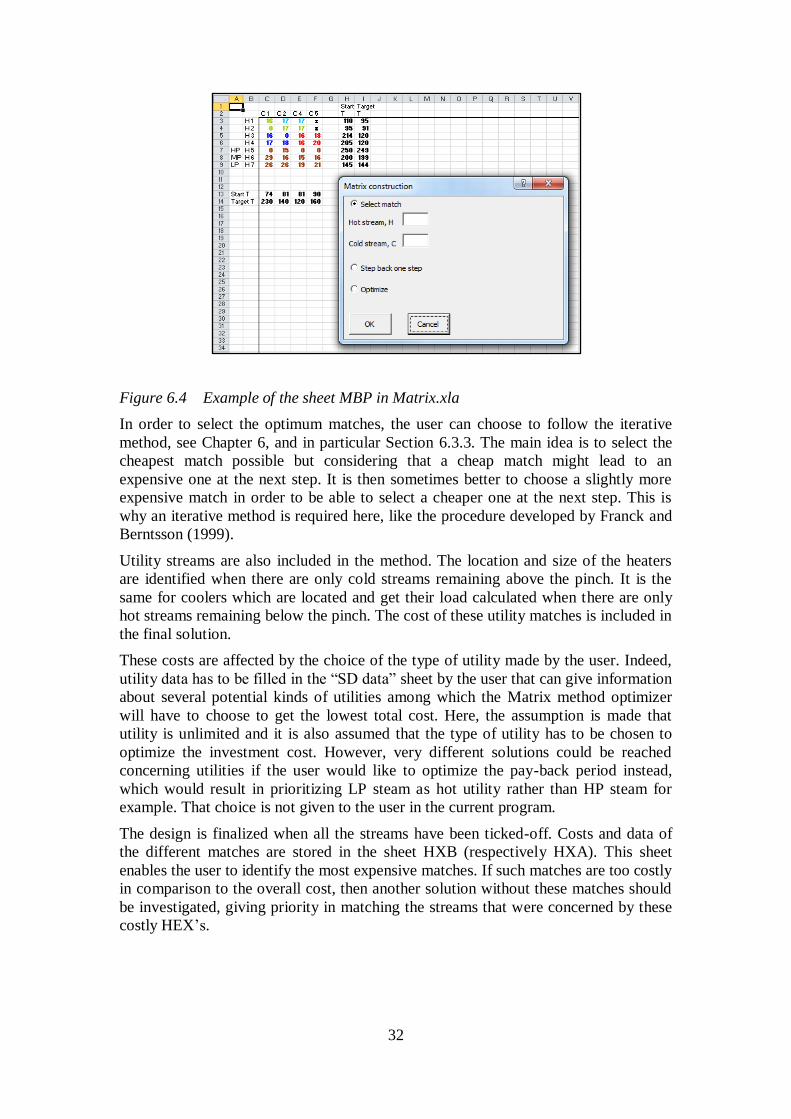
Figure 6.4 Example of the sheet MBP in Matrix.xla
In order to select the optimum matches, the user can choose to follow the iterative
method, see Chapter 6, and in particular Section 6.3.3. The main idea is to select the
cheapest match possible but considering that a cheap match might lead to an
expensive one at the next step. It is then sometimes better to choose a slightly more
expensive match in order to be able to select a cheaper one at the next step. This is
why an iterative method is required here, like the procedure developed by Franck and
Berntsson (1999).
Utility streams are also included in the method. The location and size of the heaters
are identified when there are only cold streams remaining above the pinch. It is the
same for coolers which are located and get their load calculated when there are only
hot streams remaining below the pinch. The cost of these utility matches is included in
the final solution.
These costs are affected by the choice of the type of utility made by the user. Indeed,
utility data has to be filled in the “SD data” sheet by the user that can give information
about several potential kinds of utilities among which the Matrix method optimizer
will have to choose to get the lowest total cost. Here, the assumption is made that
utility is unlimited and it is also assumed that the type of utility has to be chosen to
optimize the investment cost. However, very different solutions could be reached
concerning utilities if the user would like to optimize the pay-back period instead,
which would result in prioritizing LP steam as hot utility rather than HP steam for
example. That choice is not given to the user in the current program.
The design is finalized when all the streams have been ticked-off. Costs and data of
the different matches are stored in the sheet HXB (respectively HXA). This sheet
enables the user to identify the most expensive matches. If such matches are too costly
in comparison to the overall cost, then another solution without these matches should
be investigated, giving priority in matching the streams that were concerned by these
costly HEX’s.

33
6.3 Automated routine program
The automated routine program (Matrix method optimizer) written by Andersson
(2001) calculates the optimal solution to a retrofit problem of a HEN, that is, the most
cost effective one. The routine can shortly be described as an iterative process that
follows a defined pathway towards the most cost optimal solution. Andersson (2001)
represents the whole evaluation problem of a HEN as a tree in his thesis. The initial
cost matrix that is constructed for the HEN according to the Matrix method is referred
to as the “root node” and there is only one root node. A choice of adding/removing
heat from any stream(s) is a “pathway” towards a new constructed matrix which is a
new node. Each possible pathway from the root “branches out” as an intermediate
node and these “branch out” as terminal nodes. The pathway from a terminal node up
to the root node is defined as a complete possible solution. The further any path is
followed from the root, the higher the partial cost of the network will be until a
solution is reached. Sometimes it is impossible for any match between streams to be
selected as this is thermodynamically unfeasible, in such a situation, the program
steps back to a previous branch and tries to find another solution.
6.3.1 Matrix behavior
In the Matrix method optimizer, the rows of a matrix represent cold streams and its
columns represent hot streams which is the other way around from how a matrix is
presented in Matrix.xla (Franck och Berntsson 1999). As a match is selected, a new
possibly smaller matrix is constructed according to the following procedure:
A tick-off of a cold stream results in a new matrix with the corresponding row
taken away and new values added to the corresponding column
A tick-off of a hot stream results in a new matrix with the corresponding
column taken away and new values added to the corresponding row
No tick-off of any stream results in a new equally sized matrix with new
values added to the corresponding column and row, however the same match
cannot be selected again immediately
As the first “root node” matrix is constructed by the program, it selects a match and
registers the cost. The next matrix is then constructed and a new match is selected and
the cost for this match is added and registered to the partial cost of the solution. This
is repeated until the end of a branch is reached and no more HEX’s can be added to
the list. The end of a branch is reached either if a solution has been found or if there is
no possibility to continue, a dead-end. If a dead-end is reached, the routine takes one
step back and tries to find a solution through another branch by selecting a different
match in the previous step of the routine. This is repeated until a solution is found and
once a solution is found, that is; if all the hot streams above the pinch or all the cold
streams below the pinch are empty, the utility matches are optimized. The costs for
the utility matches are added to the partial solution cost and this will represent one
complete solution with a total cost, the end of a branch. When all the stream
combinations are checked by the program and the resultant costs are calculated, the
HEN is fully evaluated according to the Matrix method.

34
6.3.2 Optimization strategies
The Matrix method optimizer is using 5 different strategies for its cost optimization of
HEN’s to work as fast as possible.
6.3.2.1 Upper bound tree search
Once a solution has been calculated, this cost will be recorded as an upper bound limit
for the rest of a tree search. After this has been done, the optimizer steps back and
continues searching by matching streams along other branches, however if the partial
cost will reach a cost higher than that of a previous complete solution, the branch
investigation will be terminated in order to save iteration time and the optimizer steps
back once again until a new solution is possibly reached. When all the combinations
on one level have been tested, the optimizer steps back and tests all the combinations
on a previous level until all the relevant combinations have been tested. If a new
cheaper solution is found, this will be recorded as the new upper bound limit and the
search will continue as previously with this new upper bound limit in attention for
future branch search terminations, see Figure 6.5.
Figure 6.5 Example of the search strategy inside the Matrix method optimizer tool
0
0
5
5
8
5
10 13
10 11
7
20 21 20
20 30 15
40 51 > 45 : Step back 35
Utility: 5 Utility : 0
Solution = 45 Solution = 35 New Upper Bound

35
6.3.2.2 Arrangement
The construction of each new matrix involves an arrangement of the costs according
to their amount. This is done so that the optimizer selects the cheapest cost match of
each matrix first and therefore almost certainly finds a low upper bound limit as early
on in the routine as possible. The amount of iterations will be less this way and
therefore iteration time will be saved in order for the optimizer to work faster. To
understand how this is performed, see Anderson (2001), Chapter 3.2.2.
6.3.2.3 Combination check
Whenever a new matrix is constructed, only the corresponding match row and column
will be altered. Therefore multiple matches checked in any order may not affect each
other. These are called independent matches and will result in a matrix looking
exactly the same no matter the order these independent matches are chosen. A
combination check is thus implied to avoid the same calculations several times by the
program since the resulting matrix will look the same anyway. Hence, independent
matches are stored in the memory and one resulting combination of independent
matches will never be calculated more than once. This saves iteration time further.
6.3.2.4 Pinch violation check
There is a function in the optimizer routine that makes sure that “the three golden
pinch rules” are not violated. This is called temp_possible. If heating needs to be done
below the pinch or if cooling needs to be done above the pinch, temp_possible tells
the program to stop the evaluation of the matrix branch and find another branch to
work on. That can happen for example when the lowest targeted temperature of the
hot streams is lower than the lowest starting temperature of the cold streams above the
pinch. In such a case, a cold utility would be required which is a violation above the
pinch. Heating through the pinch is not considered as the problem is divided into two
parts on each side of the pinch.
6.3.2.5 Loop check
If several HEX’s are used on the same matches of streams more than once, this will
result in a rapid cost increase. Normally, the upper bound limit optimization will take
care of this problem by not letting the optimizer continue on such a branch.
Nevertheless if the first solution investigated is a branch like this and no upper bound
limit has been registered yet, iteration time may be wasted on checking such
combinations. Loop_check is therefore an optimization function that makes sure that
the optimizer does not select a match between two streams if a HEX already is
connecting them from a previous step.

36
6.3.3 Flow chart
Figure 6.6 Flow chart describing the Matrix method optimizer procedure.
Create matrix1
Function=
f(matrix)
Temp_
possible?Exit function
Sort matrix
For all
matches
Tot cost < reg
min cost?Next match
Combination
checked?Next match
Loop? Next match
Calculate new
matrix
New matrix
empty?
Optimise utility
Tot cost < reg
min cost?
Register new
min cost
Next match
Display
optimal result
No
No
No
No
No
No
Yes
Yes
Yes
Yes
Yes
Yes

37
7 Description of issues in the Matrix method, the
calculation tool and the optimizer
In the Matrix method the problem is divided into two parts by dividing the network at
the pinch point. Each problem (above and below the pinch) is then solved separately.
If the user chooses to reach a retrofitted network achieving the MER for a specific
ΔTmin then, all the pinch violations across the pinch will be rearranged. Then, no criss-
cross is allowed in the pinch region and the division of the problem into two might
result in the following issue:
A small part of a stream involved in a violation might end up on one side of the pinch
while its major part remains on the other side. In such a case, the method might use a
different HEX for each part of the stream while it would be cheaper to match this
stream with only one HEX crossing the pinch. That means that it would be cheaper to
merge the two HEX’s by allowing the small part of the stream to violate the pinch
rule.
In order to handle this issue, the current Matrix calculation tool enables the user to
choose which violations he wants to rearrange or not. That allows a more flexible
division of the network and can reduce the number of new units and extended HEX’s
required considerably, resulting in a cheaper overall solution. However, this division
will impact the energy recovery level every time a violation will be tolerated.
Moreover, there is no priority rule to handle the violations in the present Matrix
calculation tool Matrix.xla. It is up to the user to choose which violations to accept or
not. Then, a match that violates the pinch with only a small part of its total heat load
can be equal in priority for rearrangement to another HEX that violates the pinch with
its entire heat load if the user chooses so. That might lead to rearrange a complete
HEX for solving a minor violation instead of using this money for fixing a bigger
violation. The optimal choice of units to rearrange has to be identified. This is not
handled by the current calculation tool and is requiring the user’s knowledge and
experience to prioritize the violations by considering both their size and their cost per
unit of saved energy. A method developed by Carlson (1996) exists and could be
implemented in the Matrix.xla program. That step of the program could easily be
automated in order to prevent expensive retrofit solutions.
7.1 Merging the solutions above and below the pinch
The flexible division of the network described above also brings a second issue. Since
some pinch violations are allowed, it is possible that the same HEX appears in the
solutions both above and below the pinch, because the two problems are solved
independently. That has no direct consequences if it is an already existing HEX since
its cost is set to zero in this case, but it would have consequences on the final solution
if it implies a HEX with costs since the total cost is the addition of the solutions above
and below the pinch.
Consequently, the user has to compare solutions above and below the pinch to verify
if any HEX appears on both sides or if two exchangers on different sides can be put
together as one (how to know if it is possible)
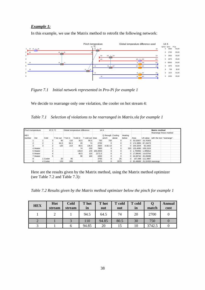
38
Example 1:
In this example, we use the Matrix method to retrofit the following network:
Figure 7.1 Initial network represented in Pro-Pi for example 1
We decide to rearrange only one violation, the cooler on hot stream 4:
Table 7.1 Selection of violations to be rearranged in Matrix.xla for example 1
Here are the results given by the Matrix method, using the Matrix method optimizer
(see Table 7.2 and Table 7.3):
Table 7.2 Results given by the Matrix method optimizer below the pinch for example 1
HEX Hot
stream
Cold
stream
T hot
in
T hot
out
T cold
out
T cold
in
Q
match
Annual
cost
1 2 1 94.5 64.5 74 20 2700 0
2 1 3 110 94.85 80.5 30 750 0
3 1 6 94.85 20 15 10 3742.5 0
Pinch temperature Global temperature difference used 14 K88 °C Qrest Qtot FCp
1 20 20 8 95 95 1 110 110 0 4500 50,00C8 V1
2 65 65 2 95 95 0 2700 90,00V2
3 120 120 3 214 214 0 2820 30,00V3
4 120 120 9 205 205 0 2975 35,00C9
5 20 20 74 74 4 230 230 0 10500 50,00V2 H4
6 81 81 137 137 5 140 140 0 2975 50,00V3 H5
7 30 31 81 8 758 15,00V1
8 81 81 6 120 120 0 2173 55,00H6
9 90 90 7 160 160 0 2450 35,00H7
Pinch temperature 87,5 °C Global temperature difference 14 K Matrix method
Rearrange those marked
HEX
number Hot Cold T hot out T hot in Tcold in T cold out Qvvx
Q through
pinch
Cooling
above
Heating
below Area UA-value with the text "rearrange".
1 1 3 95 110 30,5 80,5 750 750 0 0 33,52607 16,76303
2 2 1 64,5 94,5 20 74 2700 0 0 0 174,3895 87,19473
3 3 2 120 214 80,5 136,9 2820 -4,5E-13 0 0 100,3204 50,1602
4 Heater 1 74 230 7800 0 0 325 133,4085 109,1524
5 Heater 2 136,9 140 155,0003 0 0 0 1,705992 1,395812
6 Heater 4 80,5 120 2172,5 0 0 0 17,89045 14,63764
7 Heater 5 90 160 2450 0 0 0 24,69742 20,20698
8 1 Cooler 20 95 3750 0 25 0 167,098 111,3987
9 4 Cooler 120 205 2975 0 2975 0 30,48689 20,32459 rearrange

39
Table 7.3 Results given by the Matrix method optimizer above the pinch for example1.
HEX Hot
stream
Cold
stream
T hot
out
T hot
in
T cold
in
T cold
out
Q
match
Annual
cost
1 1 3 95 110 30.5 80.5 750 0
2 3 2 120 214 80.5 136.9 2820 0
3 4 1 120 205 74 133.5 2975 16.93208
4 5 1 249 250 133.5 230 4825 0
5 5 2 249 250 136.9 140 155 0
6 5 4 249 250 80.5 120 2172.5 0
7 5 5 249 250 90 160 2450 0
The HEX between Hot stream 1 and Cold stream 3 is present both in the solution
above and below the pinch. Since it is not a HEX that has to be rearranged and
because it already exists, its cost is equal to zero and then, the fact that it is present in
both solutions will not affect the final result.
Example 2:
In this second example, we use the exact same network as in example 1 but in
addition to the cooler on hot stream 4 we also decide to rearrange the HEX between
hot stream 1 and cold stream 3. Here are the results for both sides of the problem (see
Table 7.4 and Table 7.5):
Table 7.4 Results given by the Matrix method optimizer below the pinch for example 2
HEX Hot
stream
Cold
stream
T hot
in
T hot
out
Tcold
out
T cold
in
Q
match
Annual
cost
1 2 1 94.5 64.5 74 20 2700 0
2 1 3 95 79.85 80.5 30 757.5 12.4434
3 1 6 79.85 20 15 10 2992.5 0
Table 7.5 Results given by the Matrix method optimizer above the pinch for example 2
HEX Hot
stream
Cold
stream
T hot
out
T hot
in T cold in
T cold
out
Q
match
Annual
cost
1 3 2 120 214 80.5 136.9 2820 0
2 4 1 120 205 74 133.5 2975 16.93208
3 1 4 95 110 80.5 94.13636 750 17.20568
4 5 1 249 250 133.5 230 4825 0
5 5 2 249 250 136.9 140 155 0
6 5 4 249 250 94.13636 120 1422.5 0
7 5 5 249 250 90 160 2450 0
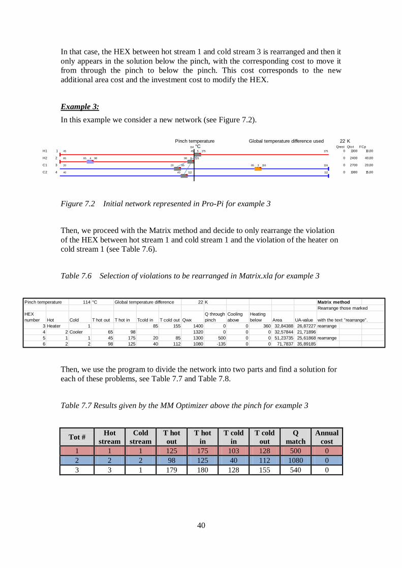
40
In that case, the HEX between hot stream 1 and cold stream 3 is rearranged and then it
only appears in the solution below the pinch, with the corresponding cost to move it
from through the pinch to below the pinch. This cost corresponds to the new
additional area cost and the investment cost to modify the HEX.
Example 3:
In this example we consider a new network (see Figure 7.2).
Figure 7.2 Initial network represented in Pro-Pi for example 3
Then, we proceed with the Matrix method and decide to only rearrange the violation
of the HEX between hot stream 1 and cold stream 1 and the violation of the heater on
cold stream 1 (see Table 7.6).
Table 7.6 Selection of violations to be rearranged in Matrix.xla for example 3
Then, we use the program to divide the network into two parts and find a solution for
each of these problems, see Table 7.7 and Table 7.8.
Table 7.7 Results given by the MM Optimizer above the pinch for example 3
Tot # Hot
stream
Cold
stream
T hot
out
T hot
in
T cold
in
T cold
out
Q
match
Annual
cost
1 1 1 125 175 103 128 500 0
2 2 2 98 125 40 112 1080 0
3 3 1 179 180 128 155 540 0
Pinch temperature Global temperature difference used 22 K114 °C Qrest Qtot FCp
H1 1 45 45 5 175 175 0 1300 10,00V5
H2 2 65 65 4 98 98 6 125 0 2400 40,00C4 V6
C1 3 20 20 85 85 3 155 155 0 2700 20,00V5 H3
C2 4 40 40 112 112 0 1080 15,00V6
Pinch temperature 114 °C Global temperature difference 22 K Matrix method
Rearrange those marked
HEX
number Hot Cold T hot out T hot in Tcold in T cold out Qvvx
Q through
pinch
Cooling
above
Heating
below Area UA-value with the text "rearrange".
3 Heater 1 85 155 1400 0 0 360 32,84388 26,87227 rearrange
4 2 Cooler 65 98 1320 0 0 0 32,57844 21,71896
5 1 1 45 175 20 85 1300 500 0 0 51,23735 25,61868 rearrange
6 2 2 98 125 40 112 1080 -135 0 0 71,7837 35,89185

41
Table 7.8 Results given by the Matrix method optimizer below the pinch for example 3
Tot # Hot
stream
Cold
stream
T hot
in
T hot
out
Tcold
out
T cold
in
Q
match
Annual
cost
1 2 2 125 98 112 40 1080 0
2 1 1 125 91 103 86 340 11,63981
3 2 1 98 65 86 20 1320 16,44882
4 1 3 91 45 25 15 460 11,91078
We can see that both HEX’s between H1-C1 and H2-C2 are present in the solutions
both above and below the pinch. This is not an issue for the HEX linking hot stream 2
to cold stream 2 because this HEX is already existing and we decided not to rearrange
it, then it will not induce costs. However, the HEX between hot stream 1 and cold
stream 1 brings issues. Indeed, above pinch it has not any cost because this HEX
already exists and does not require any changes in its area here. But, if we consider its
price below pinch, this value is calculated by considering the area changes AND the
unit capital cost. The Matrix calculation tool considers that this HEX is a different one
below pinch than the one above pinch and consequently considers that a new HEX
has to be built below pinch. Consequently, the Matrix calculation tool considers that
the final solution is as represented on Figure 7.3:
Figure 7.3 Final merged solution for example 3 as considered by the program.
In reality, the two HEX’s between H1 and C1 are the same HEX. Consequently, the
total price of the retrofitted solution should not consider any capital cost from this
HEX that already exists. The only cost that should be included is that of its area
modification. That issue is really important to fix in the Matrix calculation tool
because it means that in some situations, the additional cost generated by this mistake
can lead to avoiding this solution and choose a retrofitted network that is not the real
optimal solution.
H1
H2
C1
125ºC91ºC
125ºC65ºC
20ºC 103ºC86ºC
C
340 kW1320 kW
460 kW
45ºC
C2112ºC
1080 kW
175ºC
155ºC128ºCH
540 kW500 kW40ºC
98ºC
42
To summarize, there are mainly two issues in the current Matrix calculation tool,
arising from the separation of the network into two parts:
When a HEX is allowed to violate a pinch rule by not being retrofitted, it
might appear in both the solutions above and below the pinch. Since it is not
rearranged, such a situation will not impact the calculation of the total cost of
the final solution. The main issue here is that the user should be careful and
not forget to consider this HEX as only one when he will gather the two
solutions to get the final retrofitted network.
If the same two streams are matched above and below the pinch, the Matrix
calculation tool might generate two different HEX’s (one for both sides). That
might generate additional costs because the calculation tool will consider two
different capital costs while these HEX’s can be combined in a unique one in
the final solution. This issue requires the user to be careful when applying the
tool but it might also lead to non-optimal solutions. Indeed, the additional cost
generated by the division of this HEX into two different ones might lead the
Matrix method optimizer to consider that this solution is not the most
economical one while it should be. It is then important to try to find a way to
cope with this issue, inside the calculation tool or the optimizer itself.
7.2 How to handle stream splitting
7.2.1 Definition + Example
In some cases, a stream should be split in order for a retrofit problem to be solved or
to reduce the number of units as the unit cost is a large part of the HEX cost. Such a
case can occur when the amount of hot and cold streams with starting/ending
temperatures close to the pinch do not match each other and when the criteria for the
temperature driving forces are not met.
The criteria to be met for design at the pinch according to Kemp (2007) are as
follows:
Above the pinch: FCphot ≤ FCpcold Nhot ≤ Ncold
Below the pinch: FCphot ≥ FCpcold Nhot ≥ Ncold
F stands for mass flow of the stream (kg/s), Cp is the specific heat for the fluid in the
stream (kJ/kg.K) where hot and cold denotes whether it is for the hot or the cold
stream. N stands for the amount of stream branches at the pinch (including both split
and full streams).
A relevant example is illustrated in Figure 7.4 below where the streams of an organic
distillation are illustrated.

43
Figure 7.4 Example of network where a stream split is required.
In this situation the ΔTmin has been set to 200C and therefore it is impossible to get a
solution by interchanging HEX’s. A split of the cold stream is necessarily done as
seen in the figure in order to avoid cooling above the pinch and thus solve the MER
retrofit problem. This split is motivated due to the fact that the amount of cold streams
is less than the amount of hot streams according to the criteria above combined with
the fact that cold stream 1 has a higher FCp value.
There is an algorithm that helps the user knowing when and when not to split a stream
due to the previous criteria given. This algorithm is expressed in Figure 7.5. It does
not give answers about which stream to split and in what proportion but it can be
combined with a method from Kemp (2007) and in particular Section 4.3.1 to solve
these issues.
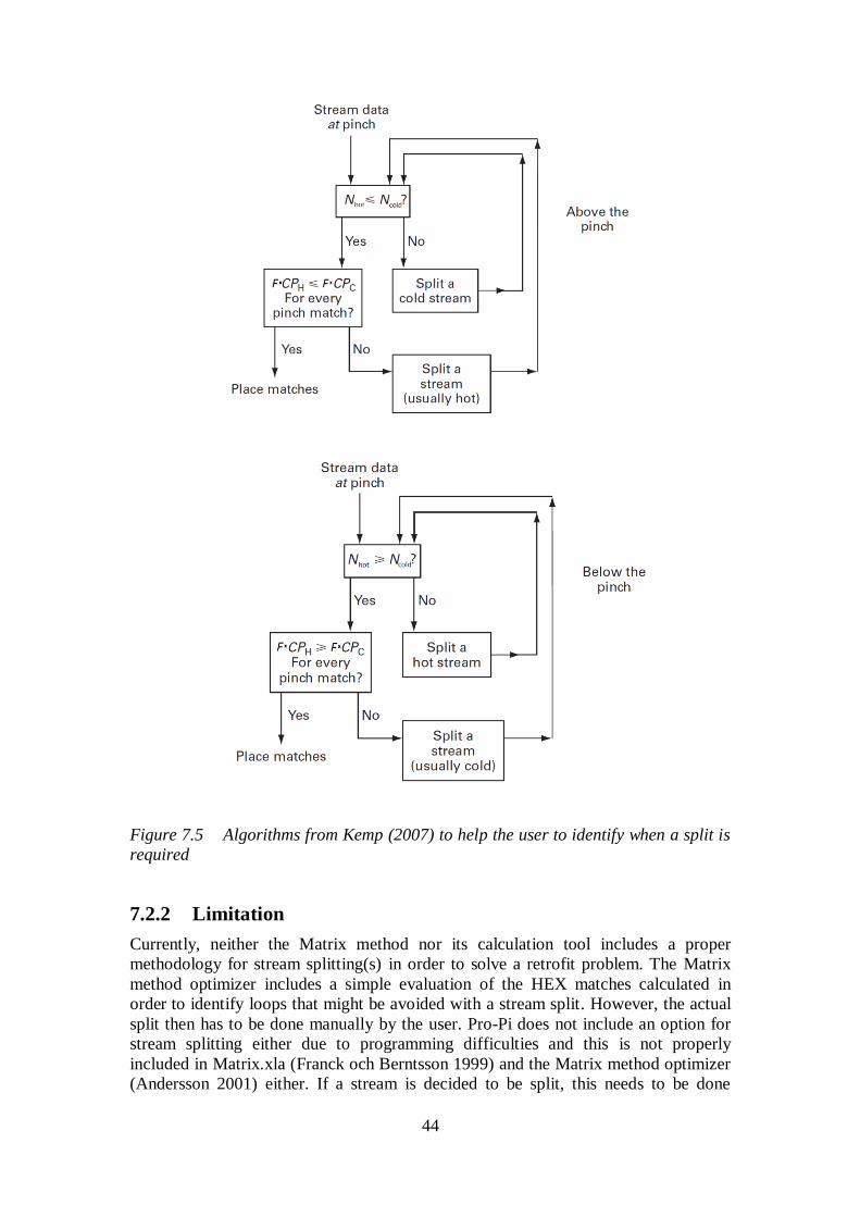
44
Figure 7.5 Algorithms from Kemp (2007) to help the user to identify when a split is
required
7.2.2 Limitation
Currently, neither the Matrix method nor its calculation tool includes a proper
methodology for stream splitting(s) in order to solve a retrofit problem. The Matrix
method optimizer includes a simple evaluation of the HEX matches calculated in
order to identify loops that might be avoided with a stream split. However, the actual
split then has to be done manually by the user. Pro-Pi does not include an option for
stream splitting either due to programming difficulties and this is not properly
included in Matrix.xla (Franck och Berntsson 1999) and the Matrix method optimizer
(Andersson 2001) either. If a stream is decided to be split, this needs to be done

45
manually by starting the process over again from the beginning and altering the input
stream data sheet for Pro-Pi. In the optimizer; if the only possible solution is to split a
stream or a cost efficient solution is a stream split, the internal function temp_possible
will terminate the branch as a stream split will not be an option and thus this solution
is left out of the final evaluation of the matrix.
Yet, the optimizer tool for Matrix.xla gives the user a hint that streams should be split
if a large occurrence of repeatedly alternating HEX’s is part of a branch result (see the
following example). This is due to the internal function named Loop_check,
previously described, that detects if there are many loops between the same two
streams in a terminated solution branch. Nevertheless, a stream split can be very cost
efficient and “in a retrofit situation the heat exchanger area, piping, and pressure drops
all influence the optimal way of splitting the stream” (Carlsson 1996). Furthermore,
Carlsson (1996) mentions in her thesis that stream splits should be included in the
Matrix method as the current approach of splitting a stream is based solely on
judgment of the ΔTlm and the temperature difference of the two sides of the relevant
HEX.
Example:
If we consider the following network (see Figure 7.6) and try to retrofit it by applying
the Matrix method with the optimization tool, we get no solution.
Figure 7.6 Initial network represented in Pro-Pi for example on stream splitting.
In the case below, non-tick-off matches have been selected between the streams C2
and H1 for example; creating loops between the two streams (see Figure 7.7)
Figure 7.7 Retrofitted solution without stream split requiring loops.
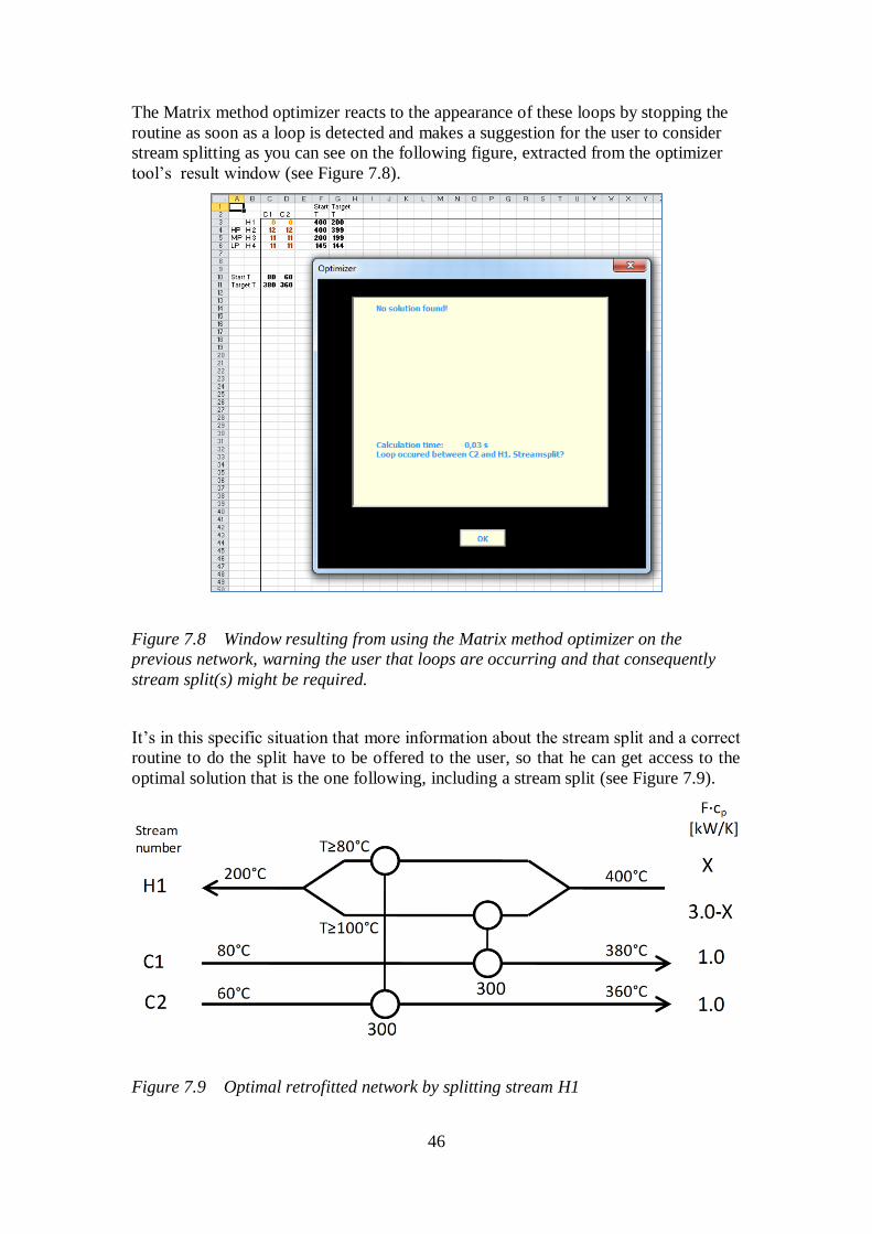
46
The Matrix method optimizer reacts to the appearance of these loops by stopping the
routine as soon as a loop is detected and makes a suggestion for the user to consider
stream splitting as you can see on the following figure, extracted from the optimizer
tool’s result window (see Figure 7.8).
Figure 7.8 Window resulting from using the Matrix method optimizer on the
previous network, warning the user that loops are occurring and that consequently
stream split(s) might be required.
It’s in this specific situation that more information about the stream split and a correct
routine to do the split have to be offered to the user, so that he can get access to the
optimal solution that is the one following, including a stream split (see Figure 7.9).
Figure 7.9 Optimal retrofitted network by splitting stream H1
47
This solution requires only two HEX’s and not any heater nor cooler and is then the
one that should be resulting from the Matrix method optimizer as the best retrofitted
solution.
7.2.3 Possible improvement
“Since the streams are organized in a matrix, it is possible to apply an approximate
stream splitting approach as suggested by Polley” (Carlsson 1996) to the Matrix
method and the optimizing tool. This could be done by implying the stream splitting
algorithm and a proper method for how to split what stream and to what extent as
described in Kemp (2007), and in particular in Section 7.2.1. Since Pro-Pi shows
difficulties in splitting streams due to programming issues, the Matrix method
optimizer could perhaps be altered to do a stream split within the optimization
calculations and then produce a new data input sheet for Pro-Pi where new streams
are represented for a stream split if this is a cost efficient solution to the retrofit
problem.
7.3 How to choose the optimum ΔTmin
To start the process of the Matrix method, the user has to decide a value of Δ
.
The tool only helps the user in this choice by providing a table referencing the pinch
violations of the existing HEX’s for a list of various possible Δ
’s that could be
inquired. The experience and knowledge of the user is required here. When the value
of the Δ
is chosen, the whole method has to be processed. Then, the whole
procedure has to be done again with a different value of Δ
in order to be able
to draw several Cost vs Energy savings curves (see Figure 5.2). These curves will
then enable the user to pick the optimum solution. Given that this is an iterative
procedure, it would be interesting to improve the Matrix calculation tool Matrix.xla to
make it able to run the complete method for a list of several values of Δ
in
order to prevent the user from having to run the complete method several times.
7.4 Improvement of the internal calculations (Costs) and
better simplifications
The main costs, like unit, piping, area and pressure drop costs are all included in the
Matrix calculation tool. However some important costs such as space requirements
and fouling are not included even though they are critical parameters in a retrofit
design.
In addition to these omissions, some costs calculated by the current Matrix calculation
tool are uncertain. The main uncertainty concerns the cost of piping. Indeed, in the
current tool when a match between two streams is identified, the program can
calculate which one of these streams is the least expensive to reroute and calculate the
cost of new piping to bring the stream up to the second one and bring it back to its
original location. This is calculated from fixed distances between the streams, though
these distances could be updated after every match. This is because if we bring a
stream next to another one for a first match and then use this stream again in a second

48
match, it may be cheaper to build new piping to bring it to the second match from the
first match location, instead of it original position. It is also important to notice that
the heat transfer correlation according to Kern (1950) is used, and to calculate the
optimum piping design considering pressure drops and pipe diameters, routines from
Coulson and Richardson (1983) are used. It may be interesting to look at these
theories and see if they can be improved with updated knowledge.
Moreover, other assumptions are made inside the program. First, Shell-and-tube heat
exchangers are assumed except for gas streams in which case ideal tube banks are
assumed. Condensation is assumed to be on the shell side, then, evaporation will be
on the tube side except when the hot stream is a liquid. It has also been chosen to
simplify the program and not to give information about the condensation of steam in
heaters. It may be interesting to consider more accurate calculations here and to give
the opportunity for the user to choose among different types of HEX’s, including plate
HEX’s, independently of the nature of the streams, in order to better fit the situation
and the network he/she has to retrofit.
Finally, the user has to specify several hard data for the different streams for the
program to calculate the costs of the different matches. It may be interesting to link
this data sheet to a database in order to help the user in this process and to keep the
values updated. Indeed, prepared constants for investment costs for HEX’s, pipes and
pumps were set in 1999. While if we consider Figure 7.10 and Table 7.9 we can see
that prices have increased by 78% for HEX’s, by for 40% pumps and by 72% for
pipes since 1999 (Chemical Engineering 2013) . These inflation rates should be used
to update the data inside the program.
Figure 7.10 Equipment indicators chart
0
100
200
300
400
500
600
700
800
900
1000
1985 1990 1995 2000 2005 2010 2015
Ind
ex v
alu
e (B
ase
valu
e fo
r ye
ars
1957
-195
9 =
10
0)
Year
Equipment Heat exchangers& tanks
Processmachinery
Pipe, valves& fittings
Processinstruments
Pumps &compressors

49
Table 7.9 Chemical Engineering Plant’s Cost Index
7.5 Hot and cold utilities?
In the current Matrix calculation tool, the location and size of the heaters (coolers) are
identified when there are only cold (hot) streams remaining above (below) the pinch.
The cost of these utilities is affected by the thermodynamic data of the utility streams
(given by the user). Several types of utility streams can be described so that the
Matrix method optimizer can choose which one is going to be the most economical to
match a specific stream with. The costs of the utility HEX’s are only calculated when
investments in new heaters or coolers are required, but these costs do not include the
costs of the utility streams themself. This is understandable because the cost of the
utility streams will not affect the process of the original Matrix method nor the final
retrofitted design since the Matrix method is based on an energy recovery target (not
an economic target). However, a certain level of energy recovery will not always give
the same economic savings depending on what kind of utility that is reduced. It is
therefore important to include the value of the utility streams within the automated
procedure in order to identify the economically best retrofit design. Thus, very
different solutions could be reached if the user would like to optimize the net annual
profit instead of the HEN cost, which, for example, could result in prioritizing LP
steam as hot utility rather than HP steam. Furthermore, by adding the cost of the
utility streams we could improve the outcome for the user by giving figures on how
much money that would be saved every year with this retrofitted network, and what
the annualized net profit or payback period would be.
Heat
exchangers
& tanks
Process
machinery
Pipe, valves
& fittings
Process
instruments
Pumps &
compressors
Electrical
equipment
Stuctural
support
& misc
1990 357,6 392,2 271,4 329,5 355,9 370,9 366,3 469,8 353,3 502,9 297,1 349,4
1991 361,3 396,9 274,8 332,9 354,5 369,1 375,4 481,1 353,8 531,0 304,2 344,7
1992 358,2 392,2 273,0 334,6 354,1 361,3 378,2 467,2 356,6 553,0 307,8 329,1
1993 359,2 391,3 270,9 341,6 352,3 357,6 385,1 467,0 358,5 572,2 310,9 339,1
1994 368,1 406,9 272,9 353,8 351,1 368,6 394,6 495,3 365,7 585,3 316,2 348,2
1995 381,1 427,3 274,3 362,4 347,6 391,5 408,7 520,7 378,0 600,8 326,9 363,7
1996 381,7 427,4 277,5 365,1 344,2 387,1 415,5 513,7 372,1 614,5 332,1 376,0
1997 386,5 433,2 281,9 371,4 342,5 385,3 424,8 532,8 371,5 632,2 331,9 377,6
1998 389,5 436,0 287,4 374,2 341,2 382,7 430,5 534,8 365,5 648,5 332,8 393,5
1999 390,6 435,5 292,5 380,2 339,9 371,2 433,6 531,6 363,5 658,5 335,8 413,1
2000 394,1 438,0 299,2 385,6 340,6 370,6 439,4 545,9 368,6 667,8 339,4 408,8
2001 394,3 437,3 302,3 385,6 341,5 363,9 439,6 548,7 362,8 683,3 341,2 414,0
2002 395,6 437,5 305,8 390,4 345,3 356,9 444,2 555,8 363,5 699,2 341,4 415,5
2003 402,0 445,1 309,3 400,6 347,3 363,6 451,7 570,7 365,7 705,4 341,6 428,6
2004 444,2 508,1 307,7 427,7 345,2 511,8 511,3 607,8 378,5 724,6 357,4 583,9
2005 468,2 543,6 305,7 444,8 347,0 513,7 519,7 624,1 381,6 752,6 372,1 584,8
2006 499,6 588,0 309,3 468,6 350,9 548,0 549,7 708,0 420,1 785,7 403,1 625,3
2007 525,4 599,4 315,1 476,8 357,0 592,1 598,3 733,6 425,3 831,2 430,5 662,6
2008 575,4 696,8 321,8 506,9 352,9 687,6 643,4 827,6 434,7 871,7 458,5 748,7
2009 521,9 615,7 327,4 492,0 346,9 558,3 598,6 760,7 397,5 897,3 461,5 629,2
2010 550,8 659,4 328,9 504,3 339,1 610,4 622,5 824,4 422,2 902,6 478,7 680,0
2011 585,7 712,9 327,5 517,1 332,4 674,7 666,7 889,2 437,8 903,6 506,3 755,0
2012 584,6 712,5 322,6 525,6 328,2 661,7 668,7 913,8 425,8 920,1 512,5 754,6
Detailed Equipment indicators
Year CEPCI Equipment Construction labor BuildingsEngineering
& supervision

50
7.6 Other small issues
Table 7.10 Description of other small issues identified.
Issue detail Category Comments
Dealing with fouling of the streams
is not included in the calculations. Model issue
Fouling can have a cost
depending on the nature of
the streams and should be
included in the model.
All solutions including loops are
automatically rejected by the
Matrix method optimizer.
Program issue
Solution including loops
should be presented as
results if they are the only
possible result.
For unpinched problems, the Pro-
Pi program puts the entire problem
above or below the pinch. This
means that if the HEN is put above
pinch and heaters or coolers are
present in the HEN, only the cooler
will count as a pinch violation.
However, heating will be a
violation as well as it is
unnecessary in this situation.
Program issue
Unpinched networks
should be handled
separately in the program
so that both cooling and
heating are considered as
violations if unnecessary.
To handle the situation where a
HEX already exists between two
streams and a second one is added
between the same streams in a
different interval separated by a
unit on one of the streams, the
program will not consider
investment costs for this second
HEX.
Program issue
A control function should
be added in the program so
that it will be able to
understand that an
additional HEX is a new
one even if these two
streams already have been
matched.
Sometimes the program calculates
a value that is 40 times larger than
expected when optimum piping is
added to a HEX or a utility HEX
match.
Calculation issue
The VBA code has to be
investigated to find the
origin of this error.
Pre entered in the sheet TD data,
the automatic values for the FCP of
the utility streams = density *
mass-flow which is false.
Calculation issue The VBA code has to be
changed.

51
Unreliable annuity factor might
appear in several situations, where
it is automatically set to zero by the
program, resulting in no annual
cost.
Calculation issue
The VBA code has to be
investigated to find the
origin of this error.
Normally, whenever there is a
pinch violation, if one does not
enter the text “rearrange” next to
that HEX in the pinch violation
sheet, that stream will not be
rearranged and thus that
temperature interval will not be
represented in the match matrix
when doing a retrofit. This is
correct. However, if a pinch
violation does not occur, but one
chooses to still not retrofit a certain
heater, cooler or HEX, it will be
retrofitted by the program anyway.
There has to be a pinch violation
occurring on a unit in order to have
the option of not rearranging it.
Program issue
The code has to be
modified so that the user
can choose not to retrofit
some units even if they do
not violate the pinch rules.
Kinds of situations run manually,
might lead the program Matrix.xla
to give a solution while some
streams still have not reached their
target temperatures. That happens
for example if you have a cold and
a hot stream above the pinch and
you decide to start by putting a
heater on the cold stream. The
program will tick-off the cold
stream and give you the final
solution without handling the hot
stream.
Program issue
A function should be
added to make sure that all
streams reached their
targeted temperature
before delivering the final
solution. Moreover, the
program should be
modified so that heaters
and coolers can be placed
anywhere in the network
and not only at the
extremities of the pinch
(see Chapter 10)

52

53
8 Merging solution
In the previous chapter describing the issues of the current Matrix method and the
calculation tool we have highlighted several issues about the merging of the solutions
above and below the pinch in order to get the final solution.
Issue1: If an already existing HEX is present in both solutions, it has no
consequences on the results because it has no cost, nevertheless a warning
should be given to the user to make him aware that this HEX is only present
one time in the final solution. The best way to handle this issue would be to
produce a unique final solution of the whole merged network.
Issue 2: If a HEX that was previously across the pinch but is now moved to
only one side of the pinch, we have to make sure that the Matrix calculation
tool doesn’t consider it as a new HEX and that its cost is only calculated from
the extended area cost and the investment cost due to the modification of the
HEX. There should not be any cost for investment in a new HEX here. More
generally, every time the area of an existing HEX is increased (even if there is
no violation) we have to make sure that the program doesn’t consider it as a
new HEX and doesn’t add the corresponding investment costs. Only the
extension of area should be added to the cost of the match.
Issue 3: If an existing HEX is present in both solutions we have to make sure
that the program won’t consider it as two HEX’s (the already existing one + a
new one). We also have to make sure that all the area available from this HEX
will be used before any additional costs of the area is calculated. Moreover, if
a new HEX is present in both solutions, it shouldn´t be considered as two new
HEX’s, but only one.
In order to better understand how the program calculates the price of the matches and
how it differs between the already existing HEX’s and the new ones, we tracked this
information inside the VBA code of Matrix.xla. The following diagram (see Figure
8.1) resumes the procedure followed by the program.

54
Figure 8.1 Diagram summing up the procedure followed by the program Matrix.xla
to evaluate the cost of a match.
In this method used by the program we can see that there is no price difference
between the cost of area that is added to an existing HEX and the cost of area for a
new HEX. Since it is not the same cost (often more costly) to invest in a new HEX
rather than extending an existing one, it would be a major improvement in the
program to make it able to make this difference. The following explains how that
easily can be implemented in Matrix.xla.
Calculate the maximum heat load of the match: 𝑄𝑚𝑎𝑥 min(𝐹𝑐 .𝐶𝑝 𝑐 . ∆𝑇𝑐;𝐹 .𝐶𝑝 . ∆𝑇 )
Is 𝐹𝑐 .𝐶𝑝 𝑐 ≠ 𝐹 .𝐶𝑝 AND 𝑥 ≠ 0 𝑥 𝑇 𝑜𝑡 𝑖𝑛 𝑇𝑐𝑜𝑙𝑑 𝑜𝑢𝑡
Calculate 𝑥 :
If we are below pinch: 𝑥 𝑥
𝑒𝑈𝐴.(
𝐹ℎ.𝐶𝑝 ℎ
−
𝐹𝑐.𝐶𝑝 𝑐)
If we are above pinch: 𝑥 𝑥 .𝑒𝑈𝐴.(
𝐹ℎ.𝐶𝑝 ℎ
𝐹𝑐.𝐶𝑝 𝑐) 𝑥 𝑥
Calculate 𝑥 :
Is 𝑥 ≠ 𝑑𝑡𝑜
(𝑤𝑖𝑡 𝑑𝑡𝑜 𝑇 𝑜𝑡 𝑜𝑢𝑡 𝑇𝑐𝑜𝑙𝑑 𝑖𝑛)
∆𝑇𝑙𝑚 𝑥 𝑑𝑡𝑜
l𝑛(𝑥 𝑑𝑡𝑜
) ∆𝑇𝑙𝑚 0 ∆𝑇𝑙𝑚 𝑥
𝑄𝑏𝑒𝑓 𝑈𝐴. ∆𝑇𝑙𝑚
𝑈𝐴 0 𝑖𝑓 𝑡 𝑒 𝐻𝐸𝑋 𝑑𝑜𝑒𝑠 𝑛𝑜𝑡 𝑎𝑙𝑟𝑒𝑎𝑑𝑦 𝑒𝑥𝑖𝑠𝑡𝑠
Is 𝑄𝑚𝑎𝑥 𝑄𝑏𝑒𝑓 > 2 AND ∆𝑇𝑙𝑚 > 0
Does the user ask to add piping costs? Cost of the match = 0
𝐶𝑜𝑠𝑡 𝑜𝑓 𝑡 𝑒 𝑚𝑎𝑡𝑐 𝑐𝐴𝑟𝑒𝑎 + 𝑟𝐴.𝐴𝑓𝑎𝑠𝑡+ 𝑐𝑝𝑡 + 𝑐𝑝𝑠+ 𝑐𝑝𝑜𝑤+ cPiping
𝑟𝐴.𝐶𝑎.𝐴𝑖𝑏 + 𝑟𝐴. (𝐴𝑓𝑎𝑠𝑡1 + 𝐴𝑓𝑎𝑠𝑡2)+ 𝑐𝑝𝑡 + 𝑐𝑝𝑠+ 𝑐𝑝𝑜𝑤+ 𝑐𝑃𝑖𝑝𝑖𝑛𝑔
NB: • rA, Ca and b are constants comming from the
sheet ”HX input” • Ai is the additional area required in the match • Afast1 is the fixed cost to modify a HEX set in ”HX
input” • Afast2 is the optional additional cost to modify a
HEX that is specific to a precise match set in the matrix in ”HX input”
• Cpt is the cost of motors inside • Cps is the cost of motors outside • Cpow is the electricity cost • cPiping is the piping cost
𝑖𝑒 𝑖𝑠 𝑡 𝑒𝑟𝑒 𝑎 𝑛𝑒𝑒𝑑 𝑓𝑜𝑟 𝑎𝑑𝑑𝑖𝑡𝑖𝑜𝑛𝑎𝑙 𝑎𝑟𝑒𝑎?
𝐶𝑜𝑠𝑡 𝑜𝑓 𝑡 𝑒 𝑚𝑎𝑡𝑐 𝑐𝐴𝑟𝑒𝑎 + 𝑟𝐴.𝐴𝑓𝑎𝑠𝑡+ 𝑐𝑝𝑡 + 𝑐𝑝𝑠+ 𝑐𝑝𝑜𝑤 𝑟𝐴.𝐶𝑎.𝐴𝑖
𝑏 + 𝑟𝐴. (𝐴𝑓𝑎𝑠𝑡1 + 𝐴𝑓𝑎𝑠𝑡2)+ 𝑐𝑝𝑡 + 𝑐𝑝𝑠+ 𝑐𝑝𝑜𝑤
NB: • rA, Ca and b are constants comming from the
sheet ”HX input” • Ai is the additional area required in the match • Afast1 is the fixed cost to modify a HEX set in ”HX
input” • Afast2 is the optional additional cost to modify a
HEX that is specific to a precise match set in the matrix in ”HX input”
• Cpt is the cost of motors inside • Cps is the cost of motors outside
• Cpow is the electricity cost

55
8.1 Difference of cost between extension area and new
heat exchanger
The current total price for area is calculated as:
𝐴. . 𝐴 + 𝐴. (𝐴 + 𝐴 )
We can consider that the area cost will stay the same for a new HEX except for that
the fixed investment cost will be different. Then in the sheet “HX input” a new
column 𝐴 should be created next to the column 𝐴 and the cost of area for a
new HEX should be calculated as:
𝐴. . 𝐴 + 𝐴. (𝐴 + 𝐴 ).
The column 𝐴 should be renamed to 𝐴 and should only represent the
investment cost for adding area on an existing HEX.
Then, the program has to know when it should pick the value 𝐴 or 𝐴 to
calculate the area cost.
That is also easy to implement since the criteria already exists in the program but is
not used properly. Indeed, in the sheet “UA data” the UA value of the existing HEX is
automatically written by the program, based on the network to be retrofitted designed
in Pro-Pi. The non-existing HEX’s have a UA value equal to zero in this sheet.
Consequently, just before the very last step in calculating the price of the match one
more step consisting of checking the UA value should be added. If UA is equal to
zero then 𝐴 should be used. If UA is higher than zero then the program should
proceed by using 𝐴 .
Here we can highlight the fact that if a partial match is chosen between two streams, it
should be stressed that two HEX’s (an existing one and a new one for example) might
be present between the same streams on the same side of the pinch, creating a loop.
Such a situation would compromise the UA criteria for the new HEX since this value
would be different from zero. Nevertheless the program uses an internal function
called “loop check” that immediately stops the routine from selecting a match
between two streams that already have a HEX connecting them. Thus, the issue
described above is not one anymore.
Moreover if the same issue occurs but with the existing HEX on the other side of the
pinch than the new HEX (between same streams again) then, this situation is handled
by the merging diagram described further in this chapter.
Here is the modified diagram taking the price difference between a new match and the
increased area of an existing HEX into account (see Figure 8.2).

56
Figure 8.2 Diagram to evaluate the cost of a match taking the price difference of a
new match and the increased area of an existing HEX into account.
Here we can also highlight the fact that there might be an issue in the calculation of
the piping cost (pumps + pipes + electricity). Indeed, the program might not consider
the additional pressure drops generated by an addition of area to an existing HEX.
This increased pressure drop might require an increase in the power of the already
existing pumps. Even if security gaps have been taken into consideration when they
were designed the first time, they might still need to be replaced by more powerful
pumps. That would have consequences on the investment price but also the running
costs of the retrofitted solution. However, this is more related to the internal
calculation issue and is not analyzed in this thesis.
Calculate the maximum heat load of the match:
𝑄𝑚𝑎𝑥 min(𝐹𝑐 .𝐶𝑝 𝑐 . ∆𝑇𝑐;𝐹 .𝐶𝑝 . ∆𝑇 )
Is 𝐹𝑐 .𝐶𝑝 𝑐 ≠ 𝐹 .𝐶𝑝 AND 𝑥 ≠ 0 𝑥 𝑇 𝑜𝑡 𝑖𝑛 𝑇𝑐𝑜𝑙𝑑 𝑜𝑢𝑡
Calculate 𝑥 :
If we are below pinch: 𝑥 𝑥
𝑒𝑈𝐴.(
𝐹ℎ.𝐶𝑝 ℎ
−
𝐹𝑐.𝐶𝑝 𝑐)
If we are above pinch: 𝑥 𝑥 .𝑒𝑈𝐴.(
𝐹ℎ.𝐶𝑝 ℎ
𝐹𝑐.𝐶𝑝 𝑐) 𝑥 𝑥
Calculate 𝑥 :
Is 𝑥 ≠ 𝑑𝑡𝑜
(𝑤𝑖𝑡 𝑑𝑡𝑜 𝑇 𝑜𝑡 𝑜𝑢𝑡 𝑇𝑐𝑜𝑙𝑑 𝑖𝑛)
∆𝑇𝑙𝑛 𝑥 𝑑𝑡𝑜
l𝑛(𝑥 𝑑𝑡𝑜
) ∆𝑇𝑙𝑛 0 ∆𝑇𝑙𝑛 𝑥
𝑄𝑏𝑒𝑓 𝑈𝐴. ∆𝑇𝑙𝑛
𝐻𝑒𝑟𝑒 𝑈𝐴 0 𝑖𝑓 𝑡 𝑒 𝐻𝑋 𝑑𝑜𝑒𝑠 𝑛𝑜𝑡 𝑎𝑙𝑟𝑒𝑎𝑑𝑦 𝑒𝑥𝑖𝑠𝑡𝑠
Is 𝑄𝑚𝑎𝑥 𝑄𝑏𝑒𝑓 > 2 AND ∆𝑇𝑙𝑛 > 0
Does the user ask to add piping costs?
Cost of the match = 0
𝐶𝑜𝑠𝑡 𝑜𝑓 𝑡 𝑒 𝑚𝑎𝑡𝑐 𝑟𝐴.𝐶𝑎.𝐴𝑖𝑏 + 𝑟𝐴.𝐴𝑓𝑎𝑠𝑡+ 𝑐𝑝𝑡+ 𝑐𝑝𝑠+ 𝑐𝑝𝑜𝑤+ cPiping
𝑖𝑒 𝑖𝑠 𝑡 𝑒𝑟𝑒 𝑎 𝑛𝑒𝑒𝑑 𝑓𝑜𝑟 𝑎𝑑𝑑𝑖𝑡𝑖𝑜𝑛𝑎𝑙 𝑎𝑟𝑒𝑎?
𝐶𝑜𝑠𝑡 𝑜𝑓 𝑡 𝑒 𝑚𝑎𝑡𝑐 𝑟𝐴.𝐶𝑎.𝐴𝑖𝑏 + 𝑟𝐴.𝐴𝑓𝑎𝑠𝑡+ 𝑐𝑝𝑡+ 𝑐𝑝𝑠+ 𝑐𝑝𝑜𝑤
Is .𝐴 ≠ 0
𝐴𝑓𝑎𝑠𝑡 𝐴𝑎𝑑𝑑 + 𝐴𝑓𝑎𝑠𝑡 𝐴𝑓𝑎𝑠𝑡 𝐴𝑛𝑒𝑤 + 𝐴𝑓𝑎𝑠𝑡

57
Now, the next step is to consider this improvement of the program and to integrate it
in the method aiming at generating the final merged solution.
8.2 Methodology to generate the final merged solution
In order to not completely change the Matrix method, we decided to keep the solving
procedure based on the splitting of the network into two parts, above and below the
pinch. Instead we developed a method based on the current one. A first solution is
found either below or above the pinch and then, the second solution is built on the
other side of the pinch. The difference from the current method is that this second
solution will be built considering the first one. These two solutions will not be
completely independent anymore.
When building the second solution, for every match investigated, the program will
first have to check if this match already exists in the previous solution. If the match
does not exists in the other side of the pinch then the program proceeds normally
except for the fact that it has to check if this match just implies an extension of area or
a new HEX. If the match already exists in the previous solution, the program has to
check if the already calculated match and the newly calculated one both are close to
the pinch. Indeed, if this is the case these matches can be merged together, but it is
also possible to have two different HEX’s working at temperatures far from the pinch,
thus, two different HEX’s are required. If the HEX’s can be merged, the program has
to check if additional area is required for this second solution, taking the fact that
some area already might have been added or still is available from the previous
solution into account. There is no need to check if this match requires a new HEX
since this additional investment cost would have been added in the first solution.
Moreover even if the user is required to consider piping costs, they should not be
added here since they already have been added in the previous solution. However, if
the match requires an increase in area in this second side of the pinch, additional
pumping costs should be calculated and added to the ones calculated in the first
solution.
Since the first solution impacts the design of the second one, this new procedure
implies a requirement to be run several times with different solutions to the network
on the first side of the pinch in order to not miss the optimal global retrofitted
solution. This increases the complexity of the solution procedure as well as the
calculation time. A compromise is to run the method at least twice, with the solution
above pinch as first solution and then with the solution below the pinch calculated
first.
Finally, the cheapest global solution will be presented to the user. This final solution
should be presented to the user as one global solution and not as two different ones.

58
8.3 Diagram of the method
In this diagram (see Figure 8.3) we assume that the improvement to differentiate the
cost of a new HEX from only additional area is integrated to the Matrix method.
Figure 8.3 Diagram of a method to provide a merged retrofitted solution.
Solve solution Above pinch
Start solving Below pinch
i=1
Is match i present in solution above pinch?
𝑇 𝑜𝑡 𝑜𝑢𝑡 𝑎𝑏𝑜𝑣𝑒 𝑇 𝑜𝑡 𝑖𝑛 𝑏𝑒𝑙𝑜𝑤 𝑇𝑐𝑜𝑙𝑑 𝑜𝑢𝑡 𝑏𝑒𝑙𝑜𝑤 𝑇𝑐𝑜𝑙𝑑 𝑖𝑛 𝑎𝑏𝑜𝑣𝑒
For this match i, do we have:
AND
Is 𝐴𝑖𝑛𝑖𝑡 𝐻𝑋 𝐴𝐻𝑋 𝑎𝑏𝑜𝑣𝑒 > 0 ?
Calculate the cost of the match as usual except that
you don’t have an investment cost for the
new HEX or the piping cost
Calculate cost of the match as usual except that you don’t have an investment cost for
the new HEX, no piping cost and
𝐴𝑖 𝐴𝑖 ( 𝐴𝑖𝑛𝑖𝑡 𝐻𝑋 𝐴𝐻𝑋 𝑎𝑏𝑜𝑣𝑒) NB: 𝐶𝑜𝑠𝑡 0 𝑖𝑓 𝐴𝑖 < 0
Calculate the cost of the match as usual with an
investment cost for the new HEX and piping cost (if required by the user)
Are all streams ticked-off?
i=i+1
Calculate the cost of the match as
usual
Save solution
Have all paths been studied?
Save the cheapest merged solution
Solve the solution below pinch (independently)
Run diagram A-0 again but for solution above pinch
Select the cheapest of the two merged solutions

59
9 Solution for stream splitting
After running the Matrix method optimizer it is possible to end up with the result “no
solution found” or “stream split?” suggesting a stream split to get a solution. So far,
no tool is implemented to help the user with splitting some streams in the network to
be retrofitted. Several situations might require a stream split to improve the retrofitted
solution or to find a solution.
9.1 The two main situations requiring splitting
The first scenario consists of the case where the user runs the Matrix method and is
unable to find any retrofitted solution for the level of heat recovery required. In such a
situation, the opportunity of stream splitting should be considered to bring at least one
correct solution to the retrofit.
The second situation is already identified in the current program. It consists of the
situation where loops appear between two streams. This kind of loops requires a lot of
units and thus, is an expensive way to solve the retrofit problem. Consequently the
Matrix method optimizer cuts off the investigation of the branches involving such
looping in HEN’s and suggests a possible stream split. Here again, an additional tool
should help the user in identifying and proceeding with the optimal stream split in
order to find an economic retrofitted solution (see example in Chapter 7, Section
7.2.2).
9.2 Using splitting instead of HEX’s requiring large areas
Stream splitting should not only be investigated when it is the only remaining way to
find a solution. It should also be considered in order to optimize the retrofit solution
from an economic point of view. Indeed, it is sometimes more expensive to invest in a
new HEX requiring a large area than to proceed with a stream split. This kind of
alternative is not included in the current Matrix method and could be an interesting
improvement.
Moreover, an alternative to stream splitting should also be investigated every time a
split is considered. This alternative consists of using a specific ∆ for some HEX’s
instead of a global one for the complete network. Using individual ∆ ’s is already
available in the current method, but it should be interesting to investigate lower values
in order to see if it would lead to a more economical solution than splitting the stream.
Indeed, by reducing the ∆ of a specific HEX by a few degrees, it can prevent the
user from the necessity of splitting a stream. However this decrease of the ∆ will
induce some additional area costs. The balance between the cost of the split and the
additional area cost should be evaluated in order to choose the cheapest option. The
size of the HEN will alter its impacting result however. Indeed, choosing a more
economic stream split in a small network instead of decreasing ∆ will have a
considerable impact on a small network. However, if the network is much larger, the
savings generated by investigating such a split will represent just a little part of the
overall retrofit cost. Consequently, investigating stream splits in situations that can be
handled in a classic way may not always be as interesting as it looks like, especially
for large networks.
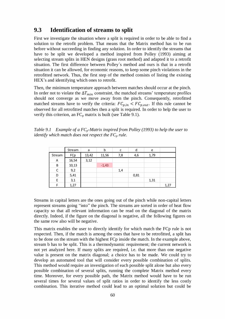
60
9.3 Identification of streams to split
First we investigate the situation where a split is required in order to be able to find a
solution to the retrofit problem. That means that the Matrix method has to be run
before without succeeding in finding any solution. In order to identify the streams that
have to be split we developed a method inspired from Polley (1993) aiming at
selecting stream splits in HEN designs (grass root method) and adapted it to a retrofit
situation. The first difference between Polley´s method and ours is that in a retrofit
situation it can be allowed, for economic reasons, to keep some pinch violations in the
retrofitted network. Thus, the first step of the method consists of listing the existing
HEX’s and identifying which ones to retrofit.
Then, the minimum temperature approach between matches should occur at the pinch.
In order not to violate the ∆ constraint, the matched streams’ temperature profiles
should not converge as we move away from the pinch. Consequently, retrofitted
matched streams have to verify the criteria: < . If this rule cannot be
observed for all retrofitted matches then a split is required. In order to help the user to
verify this criterion, an FCp matrix is built (see Table 9.1).
Table 9.1 Example of a FCp-Matrix inspired from Polley (1993) to help the user to
identify which match does not respect the FCp rule.
Streams in capital letters are the ones going out of the pinch while non-capital letters
represent streams going “into” the pinch. The streams are sorted in order of heat flow
capacity so that all relevant information can be read on the diagonal of the matrix
directly. Indeed, if the figure on the diagonal is negative, all the following figures on
the same row also will be negative.
This matrix enables the user to directly identify for which match the FCp rule is not
respected. Then, if the match is among the ones that have to be retrofitted, a split has
to be done on the stream with the highest FCp inside the match. In the example above,
stream b has to be split. This is a thermodynamic requirement; the current network is
not yet analyzed here. If many splits are required, i.e. that more than one negative
value is present on the matrix diagonal; a choice has to be made. We could try to
develop an automated tool that will consider every possible combination of splits.
This method would require an investigation of each possible split alone but also every
possible combination of several splits, running the complete Matrix method every
time. Moreover, for every possible path, the Matrix method would have to be run
several times for several values of split ratios in order to identify the less costly
combination. This iterative method could lead to an optimal solution but could be
Stream a b c d e
Stream FCp 13,42 11,56 7,8 4,6 1,79
A 16,54 3,12
B 10,13 -1,43
C 9,2 1,4
D 5,41 0,81
E 3,1 1,31
F 1,27 1,27

61
very time consuming since the complete Matrix method would have to be run many
times. Moreover in some situations, for example if there is one hot stream with a very
large FCp value, it is pretty easy to know which streams to split directly. Therefore,
instead of an automated method, an interactive one could be an alternative at this
point. The program would identify the possible splits according to the method
explained above and would present these options to the user so that he can choose
what combination of splits to go with.
9.4 Different splitting scenarios
Once the user has chosen which stream(s) to split, the program has to estimate the
cost of the retrofitted solution including the split(s). To do so, an optimal split ratio
has to be identified for every split. Different methods are possible at this point.
9.4.1 Estimation of split ratio from current network:
In some specific situations, it appears that there already is a HEX on the stream that is
going to be split and that this stream is going to be used in a match with the same
opposite stream before and after the retrofit. In that specific case, the method could
consider the existing network and use the already existing HEX on the stream that is
going to be split to calculate an optimal value of the split ratio before running the
Matrix method. The aim of this method is to make the most of the existing available
area connected to that stream while splitting it. The following example illustrates one
possible way to go for a stream already connected to two HEX’s. The original
network is presented on Figure 9.1 and the retrofitted one on Figure 9.2.
Figure 9.1 Original network before retrofit, with two HEX’s on the stream to be split
Figure 9.2 Retrofitted network with stream split
Pinch temperature Global temperature difference used 10 K65 °C Qrest Qtot FCp
200 200 3 227 227 2 300 300 1 400 400 0 600 3,00C3 V2 V1
80 80 380 380 0 300 1,00V1
60 60 280 280 4 360 360 0 300 1,00V2 H4
T1 T2
T4
T3
T5
T7
T6
T8
A1
A2

62
The aim is to identify the split ratio that minimizes the total area cost of the two
HEX’s. Given that area cost is not a linear function the optimal cost might not
correspond to the situation where A1+A2 reaches a minimum value. To find the
optimal split ratio, we have to calculate the function giving the total area cost as a
function of this ratio. In the following example, for simplification of calculations
counter flow concentric tube type HEX’s are assumed:
𝐴 ( )
∆
( )
( − )−( − )
( − −
)
(7.1)
( )
(7.2)
ℎ
ℎ
(7.3)
With
0.02
.
0.02 [
]
.
0.02 [
]
.
And
ℎ
Equations (7.1), (7.2) and (7.3) enable us to get A1 as a function of x. By using the
same calculations it is possible to get A2 as a function of x too. We can now do the
link with the area cost. If we name 𝐴 and 𝐴 the available area in HEX1 and HEX2
the cost functions are:
(𝐴 > 𝐴 𝐴 [ . (𝐴 𝐴 ) + 𝐴 ] 0) which is a function of
x.
(𝐴 > 𝐴 𝐴 [ . (𝐴 𝐴 ) + 𝐴 ] 0) which is a function of
x.
+ which is a function of x.
We can also calculate the initial areas available in the original HEX’s by using these
calculations. Indeed we cannot simply use the areas given by drawing the network in
Pro-Pi since this program only considers shell & tube type HEX’s. After the
calculation we get 𝐴 21.02 and 𝐴 1 .
.
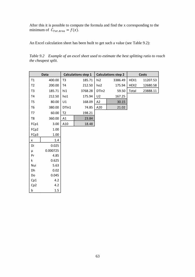
63
After this it is possible to compute the formula and find the x corresponding to the
minimum of ( ).
An Excel calculation sheet has been built to get such a value (see Table 9.2):
Table 9.2 Example of an excel sheet used to estimate the best splitting ratio to reach
the cheapest split.
Data Calculations step 1 Calculations step 2 Costs
T1 400.00 T3 185.71 hi2 3386.49 HEX1 11207.53
T2 200.00 T4 212.50 ho2 175.94 HEX2 12680.58
T3 185.71 hi1 3768.28 DTln2 59.50 Total 23888.11
T4 212.50 ho1 175.94 U2 167.25 T5 80.00 U1 168.09 A2 30.15 T6 380.00 DTln1 74.85 A20 21.02 T7 60.00 T2 198.21
T8 360.00 A1 23.84 FCp1 3.00 A10 18.48 FCp2 1.00
FCp3 1.00 x 1.4 Di 0.025 μ 0.000725 Pr 4.85 k 0.625 Nui 5.63 Dh 0.02 Do 0.045 Cp1 4.2 Cp2 4.2 b 1.5

64
If we use this calculation sheet on the previous network with the initial areas
calculated, we get the results on Figure 9.3:
Figure 9.3 Development of areas and the total cost as a function of the splitting
ratio for the retrofit of the network in Figure 9.2 using stream splitting.
In this example we can see that the total cost reaches a minimum value of 23.9 k$ for
a splitting ratio of 1.4. Areas A1 and A2 of the HEX’s stay higher than their respective
initial areas after the retrofit.
However we can have some big variations in the total cost as soon as these areas
become lower than their initial areas. For example if we consider a fictive network
just to show these possible variations, we can consider the same initial network as
before and change the initial areas (see Figure 9.4).
Figure 9.4 Development of areas and the total cost as a function of the splitting
ratio for increased initial areas of the existing HEX’s creating a fall in the HEX1 area
cost. (A10=20m2 and A20=25m
2).
23,9 15
20
25
30
35
40
45
50
55
60
1 1,2 1,4 1,6 1,8 2
Are
as a
nd
to
tal c
ost
Spliting ratio x
Development of areas and the total cost as a function of the splitting ratio
A1 (m2)
A2 (m2)
Ctot (k$)
A10 (m2)
A20 (m2)
18,39 15
20
25
30
35
40
45
50
55
60
1 1,2 1,4 1,6 1,8 2
Are
as a
nd
to
tal c
ost
Spliting ratio x
Development of areas and the total cost as a function of the splitting ratio
A1 (m2)
A2 (m2)
Ctot (k$)
A10 (m2)
A20 (m2)

65
In this situation we can see that the minimum cost is 18.39 k$ and this is reached for a
splitting ratio close to 1.8. This value corresponds to the ratio where the required area
A1 for HEX1 becomes lower than the already available area A10. At this ratio, the area
cost of HEX1 falls to 0 which explains the fall of the total cost. Then, the cost of the
area for HEX1 stays at 0 but the area cost for HEX2 continues to rise for increased
values of x, which explains the increasing total cost after the sharp fall.
The same phenomenon can be observed for the other HEX if we modify the initial
areas again (see Figure 9.5).
Figure 9.5 Development of areas and the total cost as a function of the splitting
ratio for increased initial areas of the existing HEX’s creating a fall in the HEX2 area
cost. (A10=18m2 and A20=30m
2).
In this situation we have used more points close to the sharp rise in cost to show that
this happens exactly when the required area A2 for HEX2 becomes higher than the
available one A20, i.e. at the intersection of the two curves. In this situation the
optimum cost is 11.50 k$ and is reached for a splitting ratio of 1.4.
By using this method we make sure that the split ratio will optimize the cost of the
split. Then the Matrix method can be run as usually except for that the split cost will
have to be added at the end. This method makes sure to get a solution and it gives a
way to try to minimize the total price induced by the split. However since the Matrix
method is run afterwards, some area changes might appear on the HEX present on the
split stream, or some new HEX’s might appear on this same stream. That means that
at this point the selected value for the split ratio might not be optimal.
Moreover this method is easy to run when the stream to be split already is connected
to at least two HEX’s. But it is also required to investigate how to fix the split ratio if
only one or no HEX is connected to the stream to be split. Another issue of this
method is that the matching of the streams to be split is locked.
11.50
5
15
25
35
45
55
1 1,2 1,4 1,6 1,8 2
Are
as a
nd
to
tal c
ost
Spliting ratio x
Evolution of areas and total cost as a function of splitting ratio
A1 (m2)
A2 (m2)
Ctot (k$)
A10 (m2)
A20 (m2)

66
9.4.2 Iterative method
Another method to handle the stream splits can be based on an iterative process. As
before, if the user cannot manage to get a solution, if an advice is given for splitting
(because of looping) or if the user estimates that a splitting could be beneficial, the
Matrix method optimizer has to be run again. The code should be modified so that
every time the Matrix method optimizer has been run a window asks the user if he
wants to keep this solution (if there is one) or if wants to run the optimizer again to
investigate stream splitting.
If the user chooses to investigate stream splitting, the original network that has just
been retrofitted should be saved by the program in order to be able to remember the
original matches and corresponding areas between the streams. Then, the user can
build a new network in the Pro-Pi sheet without connecting the stream to be split to
any HEX. Then the user runs the Matrix method optimizer on this network. Here
again the code of the current optimizer has to be modified so that every time a match
involving a split stream is investigated, the program has to check if this match was
already present in the network that has been saved previously. If it is the case then the
program has to check if the area required by this match is higher than the one already
present in the network previously saved. If additional area is required, it’s cost should
be added in the cost of the match. That process has to be run for several values of x
until the user gets a solution that fulfills his requirements.
In order to automatize this method, the code could be written so that the user doesn’t
have to re-draw a new network in Pro-Pi for every splitting ratio investigated. Instead,
the FCp values could be automatically changed at every iteration in the TD data sheet.
Indeed, this sheet is the one used by the Matrix method optimizer and is built from the
Pro-Pi network. Modifying TD data directly enables the optimizer to run
automatically for every splitting ratio without asking the user to draw a new network.
One advantage of this method is that the split streams do not have to be matched with
the streams it was matched with before (as it was required in first method). They can
be matched with any other stream. The optimizer will then compare this match with
the saved ones to see if that match existed in the original network or not in order to
adapt the calculation of the cost according to the area available or not. The following
diagram describes this iterative method (see Figure 9.6):
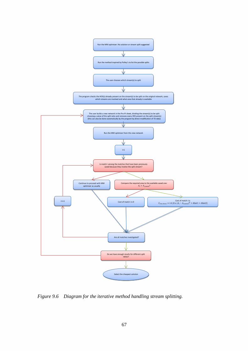
67
Figure 9.6 Diagram for the iterative method handling stream splitting.
Run the MM optimizer: No solution or stream split suggested
Run the method inspired by Polley’s to list the possible splits
The user chooses which stream(s) to split
The program checks the HEX(s) already present on the stream(s) to be split on the original network, saves
which streams are involved and what area that already is available
The user builds a new network in the Pro-Pi sheet, dividing the stream(s) to be split choosing a value of the split ratio and removes every HEX present on the split stream(s) (this can also be done automatically by the program by direct modification of TD data)
Run the MM optimizer from this new network
i=1
Is match i among the matches that have been previously saved because they involve the split stream?
Continue to proceed with MM
optimizer as usually Compare the required area to the available saved one:
𝐴𝑖 > 𝐴𝑖 𝑠𝑎𝑣𝑒𝑑?
Cost of match i is 0 𝐶𝑇𝑜𝑡 𝐴𝑟𝑒𝑎 𝑖 𝑟𝐴. [𝐶𝑎. (𝐴𝑖 𝐴𝑖 𝑠𝑎𝑣𝑒𝑑)
𝑏 +Afast1 + Afast2] Cost of match i is:
Are all matches investigated?
i=i+1
Do we have enough results for different split ratios?
Select the cheapest solution

68
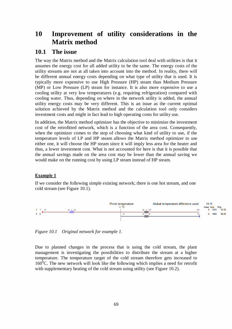
69
10 Improvement of utility considerations in the
Matrix method
10.1 The issue
The way the Matrix method and the Matrix calculation tool deal with utilities is that it
assumes the energy cost for all added utility to be the same. The energy costs of the
utility streams are not at all taken into account into the method. In reality, there will
be different annual energy costs depending on what type of utility that is used. It is
typically more expensive to use High Pressure (HP) steam than Medium Pressure
(MP) or Low Pressure (LP) steam for instance. It is also more expensive to use a
cooling utility at very low temperatures (e.g. requiring refrigeration) compared with
cooling water. Thus, depending on where in the network utility is added, the annual
utility energy costs may be very different. This is an issue as the current optimal
solution achieved by the Matrix method and the calculation tool only considers
investment costs and might in fact lead to high operating costs for utility use.
In addition, the Matrix method optimizer has the objective to minimize the investment
cost of the retrofitted network, which is a function of the area cost. Consequently,
when the optimizer comes to the step of choosing what kind of utility to use, if the
temperature levels of LP and HP steam allows the Matrix method optimizer to use
either one, it will choose the HP steam since it will imply less area for the heater and
thus, a lower investment cost. What is not accounted for here is that it is possible that
the annual savings made on the area cost may be lower than the annual saving we
would make on the running cost by using LP steam instead of HP steam.
Example 1
If we consider the following simple existing network; there is one hot stream, and one
cold stream (see Figure 10.1).
Figure 10.1 Original network for example 1.
Due to planned changes in the process that is using the cold stream, the plant
management is investigating the possibilities to distribute the stream at a higher
temperature. The temperature target of the cold stream therefore gets increased to
1600C. The new network will look like the following which implies a need for retrofit
with supplementary heating of the cold stream using utility (see Figure 10.2).

70
Figure 10.2 Network to be retrofitted due to increased targeted temperature of cold
stream.
If we run the Matrix method, using the optimizer tool, we get the following solution
(see Figure 10.3):
Figure 10.3 Retrofitted network using the current Matrix method optimizer tool.
The heater is using HP steam. If we proceed to the same retrofit using the manual
matrix method calculation tool, when we get to the final step of choosing the utility
for the heater we end up with the following matrix. We have three different hot utility
levels: LP, MP and HP steams (see Table 10.1):
Table 10.1 Description of the different utility streams available.
Here is the matrix evaluating the possibilities to tick-off the cold stream (see Table
10.2).
Table 10.2 Matrix generated in the Matrix calculation tool, estimating the cost of
ticking-off the cold stream with the different levels of utility.
Utility SD data
Name Type T T DT h
°C °C K kW/m2K
HP Hot 250 249 0,5 4,5
MP Hot 200 199 0,5 4,5
LP Hot 145 144 0,5 4,5
CW Cold 10 15 0,5 2
Q = 2100 kW

71
Generally, the rows of the matrix represents the hot streams to be retrofitted with cost
alternatives depending on with which streams they can be matched, and with their
corresponding starting and ending temperatures (0C). The column(s) of the matrix
represents the cold stream(s) to be retrofitted with match costs, including starting and
ending temperatures (0C).The costs are all alternatives (in k$) for ticking of the cold
stream 1 (C1) with the three different levels of utility available (HP, MP and LP). This
cost includes the fixed annual HEX investment cost, the pump costs, the electricity
cost (for running the pumps), the area cost and the piping costs. The price differences
are not very sharp because the fixed annual investment cost to buy the heater (10
k$/year) is much higher than the other costs. However if we focus on the decimals, we
can see that MP is significantly more expensive than HP, and LP is more expensive
than HP. The Matrix method optimizer only considers the prices in this matrix which
explains why it chooses the HP steam.
However, if we consider the cost of steam, we can assume that LP steam costs 15
$/MWh, MP steam costs 20 $/MWh and HP steam costs 30 $/MWh and if we
consider that the annual operation time is around 6000 hrs/year we can estimate the
total annual cost for the heater and utility as:
+
With being the cost for the match according to the Matrix method and
𝐴 (8.1)
We can estimate the new total cost for HP and MP steam utilities (LP steam is not
interesting in this case since it cannot tick-off the cold stream completely). Moreover,
since steam price is based on a current value, we have to consider the inflation of
prices for HEX’s, piping and pumps (see Chapter 7.4). In order to simplify the
calculations, we consider an average inflation of 78% on investment costs,
corresponding to HEX’s inflation rate:
11. 1 1. + 2.1 000
.0 (8.2)
1 .1 1. + 2.1 000
2 . 1 (8.3)
Consequently, considering the utility stream’s cost it is more economical to choose
the MP utility even if the investment cost is higher than the HP utility’s one.
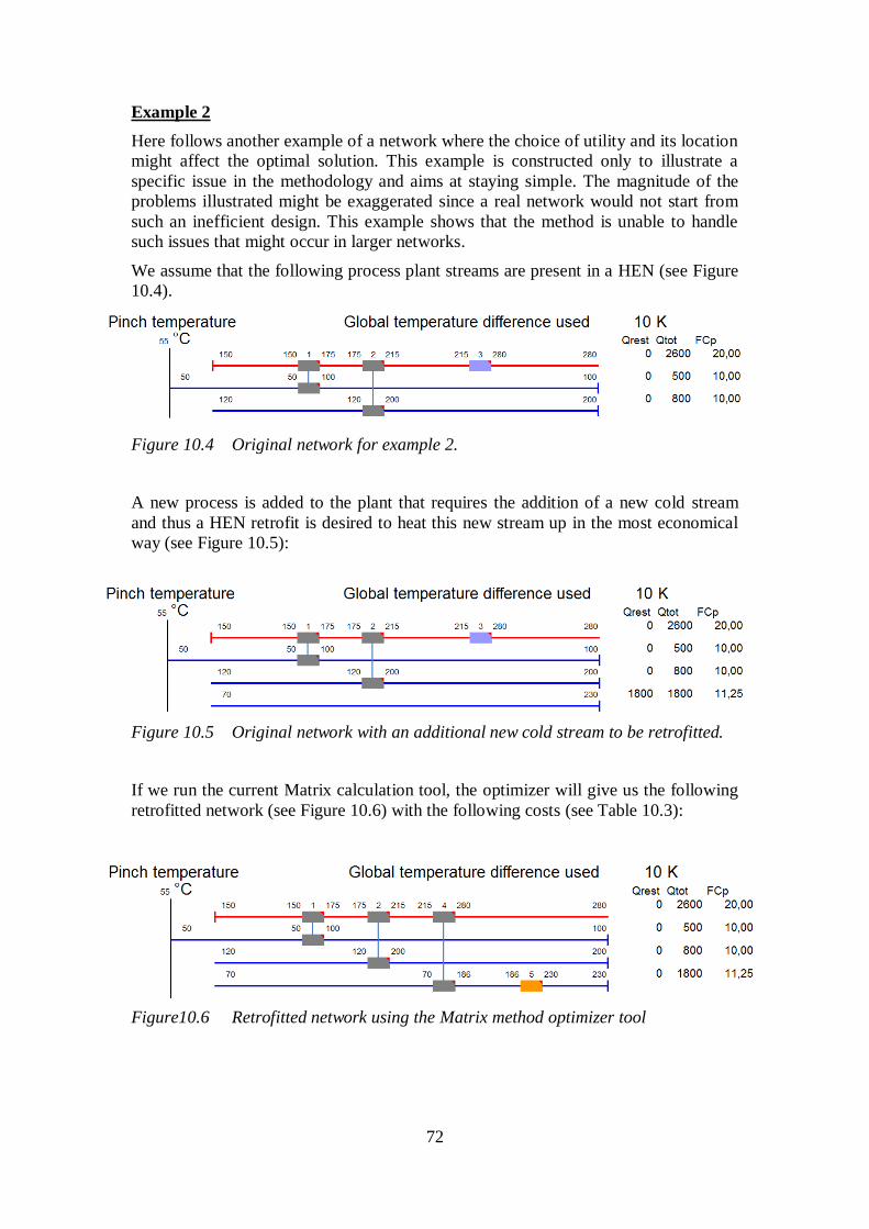
72
Example 2
Here follows another example of a network where the choice of utility and its location
might affect the optimal solution. This example is constructed only to illustrate a
specific issue in the methodology and aims at staying simple. The magnitude of the
problems illustrated might be exaggerated since a real network would not start from
such an inefficient design. This example shows that the method is unable to handle
such issues that might occur in larger networks.
We assume that the following process plant streams are present in a HEN (see Figure
10.4).
Figure 10.4 Original network for example 2.
A new process is added to the plant that requires the addition of a new cold stream
and thus a HEN retrofit is desired to heat this new stream up in the most economical
way (see Figure 10.5):
Figure 10.5 Original network with an additional new cold stream to be retrofitted.
If we run the current Matrix calculation tool, the optimizer will give us the following
retrofitted network (see Figure 10.6) with the following costs (see Table 10.3):
Figure10.6 Retrofitted network using the Matrix method optimizer tool

73
Table 10.3 Cost summary for the retrofitted solution presented in Figure 10.6
Table10.3 shows the result given by the Matrix method optimizer. The annual specific
cost describes the annual cost for each kW installed. The annual cost is the annual
investment cost based on an annuity factor of 0.25, added with the annual running
costs that include the operation cost of the electricity for driving the motor and the
pumps (does not include utility stream cost). The investment cost is based on the fixed
costs for purchasing/retrofitting a HEX added with the additional HEX area and motor
costs. Note that the piping costs are excluded in this example.
The total annual cost is 22.78 k$/year (investment without piping + running costs). If
we add the price of HP steam, assuming an annual operation time of 6000 hours, and
if we consider the increase in process equipment costs (see Section 7.4) we get a total
annual cost of:
22. 1. + 0. 000
1 0. 0 (8.4)
We can decide to place the heater close to the pinch instead of using it at the hot end
of the cold stream. Doing this allows us to use LP steam as a utility stream instead of
HP steam. Such a design is not investigated by the current optimizer but we managed
to run this configuration manually by dividing cold stream 3 into two parts just for the
calculations. The first part goes from 70 to 114oC for the heater and a second part
from 114 to 230oC for the HEX matched with hot stream 1. The results are shown in
the following figures (see Figure 10.7).
Tot annual cost 22.780 k$/year 90.360 k$ 0.190
k$/year
HEX Hot
stream Cold
stream T hot out T hot in T cold in T cold out Q match
Annual specific cost
Annual cost Investment Annual
operation
1 H1 C1 150.000C 175.00
0C 50.00
0C 100.00
0C 500 kW 0 0 0 0
2 H1 C2 175.000C 215.00
0C 120.00
0C 200.00
0C 800 kW 0 0 0 0
3 H1 C3 215.000C 280.00
0C 70.00
0C 185.56
0C 1300 kW 8.739 $/kW 11.361 k$/year 44.939 k$ 0.126 k$/year
4
H2
(HP steam)
C3 249.000C 250.00
0C 185.56
0C 230.00
0C 500 kW 22.840 $/kW 11.420 k$/year 45.421 k$ 0.065 k$/year

74
Figure 10.7 Network with cold stream 3 divided into two streams to run
calculations.
The network above actually represents the network shown below (see Figure 10.8):
Figure 10.8 The real network investigated, without representing cold stream 3 by
two separated streams.
As described previously, the bottom cold stream in the network is represented by two
different streams. This is due to the current heuristics of the Matrix calculation tool
which doesn’t allow a HEX to exchange heat far away from the pinch before heat has
been exchanged close to the pinch.
In order to implement this possibility to place heaters close to the pinch, new
heuristics are required. Indeed, if we place a heater before a HEX, we need to know
how large it should be. The tick-off rule that is normally used is not relevant in this
case. Here it is easy to say that Qheater should be Qh,min, but in a larger network with
several heaters it will be more complex.
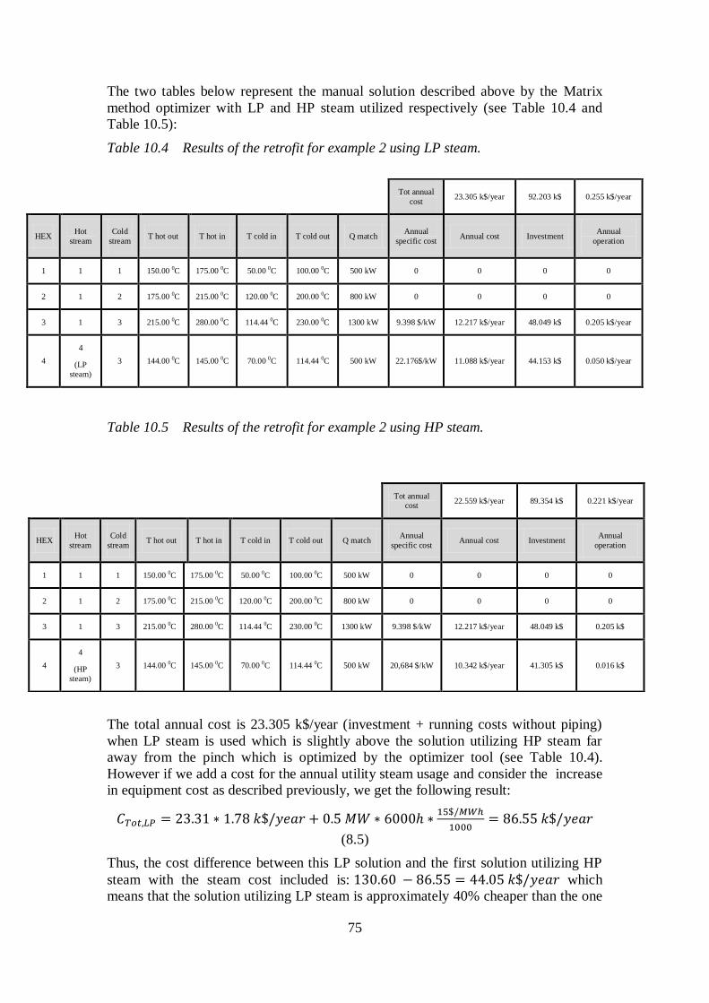
75
The two tables below represent the manual solution described above by the Matrix
method optimizer with LP and HP steam utilized respectively (see Table 10.4 and
Table 10.5):
Table 10.4 Results of the retrofit for example 2 using LP steam.
Table 10.5 Results of the retrofit for example 2 using HP steam.
The total annual cost is 23.305 k$/year (investment + running costs without piping)
when LP steam is used which is slightly above the solution utilizing HP steam far
away from the pinch which is optimized by the optimizer tool (see Table 10.4).
However if we add a cost for the annual utility steam usage and consider the increase
in equipment cost as described previously, we get the following result:
2 . 1 1. + 0. 000
.
(8.5)
Thus, the cost difference between this LP solution and the first solution utilizing HP
steam with the steam cost included is: 1 0. 0 . .0 which
means that the solution utilizing LP steam is approximately 40% cheaper than the one
Tot annual
cost 22.559 k$/year 89.354 k$ 0.221 k$/year
HEX Hot
stream
Cold
stream T hot out T hot in T cold in T cold out Q match
Annual
specific cost Annual cost Investment
Annual
operation
1 1 1 150.00 0C 175.00 0C 50.00 0C 100.00 0C 500 kW 0 0 0 0
2 1 2 175.00 0C 215.00 0C 120.00 0C 200.00 0C 800 kW 0 0 0 0
3 1 3 215.00 0C 280.00 0C 114.44 0C 230.00 0C 1300 kW 9.398 $/kW 12.217 k$/year 48.049 k$ 0.205 k$
4
4
(HP
steam)
3 144.00 0C 145.00 0C 70.00 0C 114.44 0C 500 kW 20,684 $/kW 10.342 k$/year 41.305 k$ 0.016 k$
Tot annual
cost 23.305 k$/year 92.203 k$ 0.255 k$/year
HEX Hot
stream
Cold
stream T hot out T hot in T cold in T cold out Q match
Annual
specific cost Annual cost Investment
Annual
operation
1 1 1 150.00 0C 175.00 0C 50.00 0C 100.00 0C 500 kW 0 0 0 0
2 1 2 175.00 0C 215.00 0C 120.00 0C 200.00 0C 800 kW 0 0 0 0
3 1 3 215.00 0C 280.00 0C 114.44 0C 230.00 0C 1300 kW 9.398 $/kW 12.217 k$/year 48.049 k$ 0.205 k$/year
4
4
(LP
steam)
3 144.00 0C 145.00 0C 70.00 0C 114.44 0C 500 kW 22.176$/kW 11.088 k$/year 44.153 k$ 0.050 k$/year
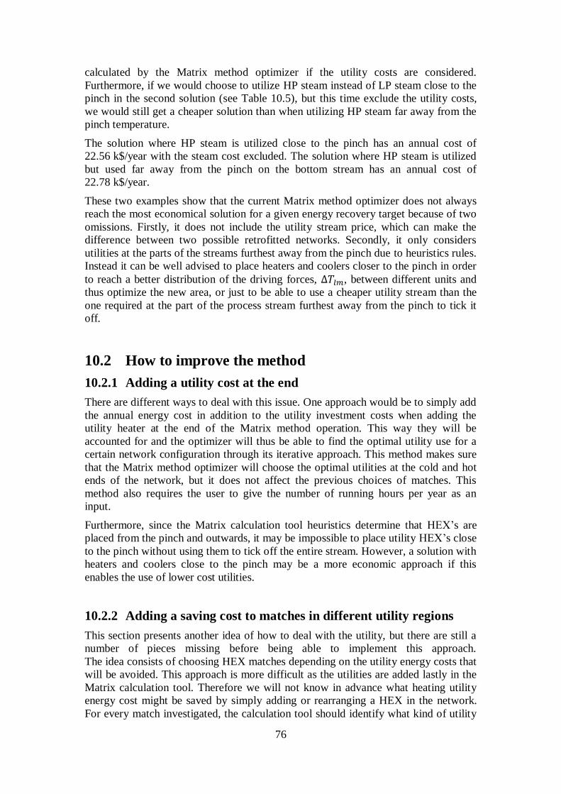
76
calculated by the Matrix method optimizer if the utility costs are considered.
Furthermore, if we would choose to utilize HP steam instead of LP steam close to the
pinch in the second solution (see Table 10.5), but this time exclude the utility costs,
we would still get a cheaper solution than when utilizing HP steam far away from the
pinch temperature.
The solution where HP steam is utilized close to the pinch has an annual cost of
22.56 k$/year with the steam cost excluded. The solution where HP steam is utilized
but used far away from the pinch on the bottom stream has an annual cost of
22.78 k$/year.
These two examples show that the current Matrix method optimizer does not always
reach the most economical solution for a given energy recovery target because of two
omissions. Firstly, it does not include the utility stream price, which can make the
difference between two possible retrofitted networks. Secondly, it only considers
utilities at the parts of the streams furthest away from the pinch due to heuristics rules.
Instead it can be well advised to place heaters and coolers closer to the pinch in order
to reach a better distribution of the driving forces, ∆ , between different units and
thus optimize the new area, or just to be able to use a cheaper utility stream than the
one required at the part of the process stream furthest away from the pinch to tick it
off.
10.2 How to improve the method
10.2.1 Adding a utility cost at the end
There are different ways to deal with this issue. One approach would be to simply add
the annual energy cost in addition to the utility investment costs when adding the
utility heater at the end of the Matrix method operation. This way they will be
accounted for and the optimizer will thus be able to find the optimal utility use for a
certain network configuration through its iterative approach. This method makes sure
that the Matrix method optimizer will choose the optimal utilities at the cold and hot
ends of the network, but it does not affect the previous choices of matches. This
method also requires the user to give the number of running hours per year as an
input.
Furthermore, since the Matrix calculation tool heuristics determine that HEX’s are
placed from the pinch and outwards, it may be impossible to place utility HEX’s close
to the pinch without using them to tick off the entire stream. However, a solution with
heaters and coolers close to the pinch may be a more economic approach if this
enables the use of lower cost utilities.
10.2.2 Adding a saving cost to matches in different utility regions
This section presents another idea of how to deal with the utility, but there are still a
number of pieces missing before being able to implement this approach.
The idea consists of choosing HEX matches depending on the utility energy costs that
will be avoided. This approach is more difficult as the utilities are added lastly in the
Matrix calculation tool. Therefore we will not know in advance what heating utility
energy cost might be saved by simply adding or rearranging a HEX in the network.
For every match investigated, the calculation tool should identify what kind of utility

77
that will be reduced by using this match and by quantifying it. Then, the cost saved by
reducing the utility demand will be reduced from the match cost as a saving cost. By
using this method we make sure that the Matrix method optimizer will make the most
economic choice at every step and will not go through match paths that would
eventually be costly because of high final utility costs. Consequently, this method
optimizes the choice of utilities but it also reduces the iteration time (because of the
upper boundary limit).
One way to use this technique inside the Matrix method is to assign specific price
boundaries to the network corresponding to the utility that is demanded. Then, every
cold stream will be associated to a cost for the zone in between these boundaries, a
cost that corresponds to the relevant hot utility that is demanded for this zone. During
the matrix process, every time a match is chosen, the price of heat load saved by this
match will be deduced from the match´s cost. The following equation describes the
cost of a match according to this approach:
𝐴. . 𝐴 + 𝐴. (𝐴 1 + 𝐴 2) + + + +
𝐴
(8.6)
Corresponding issues by using this approach:
There will be merging issues between the zones (for example; if a cold stream
passes through 2 heating zones, should it assign to a utility price
corresponding to the more expensive zone assigned to one heater installed or
will it be cheaper to install two heaters with two different utility levels?)
This method does not represent the real cost of the match, it is just here to help
the method to find the optimal path
There may be a situation where a heater already exists and uses HP utility in
the MP zone for example. How will this be handled in the calculation of the
saving costs?
10.2.3 Several solutions on a divided network
Another way to improve the true utility cost is to divide the HEN into as many parts
as there are hot utility levels instead of just dividing it at the pinch. When utility
streams are added to the HEN there will be several pinches added which the HEN gets
divided by. Then, we run the Matrix method on each and every one of these parts of
the network. When running the Matrix method, every zone will only be able to use its
own level of hot/cold utility if heaters or coolers are required and the utility will in
this case be added at the end of the Matrix methodology operations with both the
investment and the corresponding annual utility cost.

78
Corresponding Issues:
-It will be difficult to divide the network into more than two parts inside the program
-There will be increased merging issues to get the final solution
-We might end up with several heaters of different energy levels while it would be
cheaper to only use one at the highest energy level to reduce the investment cost. The
economic balance between investment and running costs should be included here.
10.2.4 Including the utility streams inside the network as soft
streams
In this approach, utility streams are included in the network as normal streams, except
that they cannot be ticked-off. The program is allowed to use them in order to tick-off
process streams, but it should not try to tick-off the utility streams. Utility streams
have soft target temperatures that don’t have to be reached to solve the network.
Consequently, utilities will not be considered only at the cold and hot ends of the
network. If they bring a cheap solution close to the pinch, a heater might be used
instead of adding a new HEX for example. The cost of the utility stream also has to be
included here, depending on the location of the heater on the stream. In this method
the utility streams will have to be identified as soft streams from the beginning. By
soft streams we mean streams that have soft ending temperatures, that is that these
temperatures do not need to be reached in order to solve the network and should thus
not be prioritized for usage. The Matrix method optimizer would then be run on hot
streams (that have to be cooled), cold streams (that have to be heated) and soft
streams (that can be used to heat or cool other streams but should not be prioritized).
Issues:
-We have to make sure that the program will not try to use more heat from utility
streams than desired/required (Qh,min)
-New heuristics might be required for placing the matches.
-How should the soft streams be handled in the computer program?
-We still have to include the cost of the utility streams (as a cost this time)
79
11 Conclusion
This thesis brings a better understanding of the Matrix method itself and the manual
matrix calculation tool program used to run this method including the Matrix method
optimizer tool after a thorough investigation and evaluation. The logics of the method
and the programs are explained and analyzed. Several issues are pointed out, among
which the merging issue, the stream splitting issue and the utility issue are the subjects
of a deeper analysis. Improvements have been identified for every one of these issues
where solutions have been developed and presented.
This research is mostly based on the previous work of Carlsson (1996), Andersson
(2001) and Franck (2010) and aims at developing the missing parts in their works to
improve the working area of the Matrix method.
Merging issues refer to the merging of the network above and below the pinch, a step
which has not yet been included in the Matrix method optimizer routine. A complete
solution to handle merging issues is presented. This solution is based on the current
program and is able to bring a final retrofitted solution for the complete network.
Stream splitting is not handled by the Matrix method today. Given the complexity of
stream splitting issues, no perfect solution is presented. Improvements are given to
solve simple situations such as the case where the stream to split is connected to at
least two HEX’s in the existing network. A method is also introduced, helping the
user to identify the situations where a split is required, and an iterative method brings
a general solution. This last method improves the current method considerably; then
again it cannot always lead to the best retrofitted network.
Finally, a major improvement is introduced by considering costs of utility streams. A
simple and easy method to implement is described to consider these costs.
Nevertheless, other methods are also suggested to handle the utilities in a better way
by allowing them to be placed anywhere in the network and not only at the extremities
of the pinch. These utility consideration methods describe the potential gain of such
solutions but they also rise additional difficulties that are not all overcome in this
thesis.
Still, a good overview of the issues with the Matrix method and the program is
presented and the suggested implementations give a good foundation for further
research work and program enhancements.
Finally, the main issues of the Matrix method have been addressed and even if the
methods proposed to solve them cannot always reach the optimal solution or handle
every situation, they definitely increase the application area of the method and enable
it to reach better solutions than previously.

80
81
12 Suggestions for future work
The solutions presented have not been implemented in the program code since this
was not in the scope of the thesis work, which directly results in the fact that no real
tests of the suggested methods could be performed on real scenario networks.
Furthermore, some of the methods suggested are left incomplete due to the
complexity of adapting them to all different kind of networks.
The next step would be to write the code to include the solutions developed for
merging and utilities. However, some research work remains to be pursued before
writing the code for stream splitting if an ideal stream splitting solution is desired. If a
general solution for stream splitting is enough, it may be implemented by following
this thesis advice. Furthermore, there should be an investigation of how interesting it
is to perform a stream split on a network if there already is another way of presenting
a solution. For instance, if it is possible to get a solution by looping HEX’s or by
lowering the ΔTmin, the solution should be compared to the optimal stream split in
order to evaluate the economic effect on the HEN.
Another future work can also be to fix all the small bugs and calculation errors inside
the current program and to improve the accuracy of the input data such as the area
cost of HEX’s.

82

83
13 Bibliography
Andersson. Routine for automatic optimisation of heat exchanger networks with the
matrix method. Master Thesis, Göteborg: Department of heat and power
technology, Chalmers University of Technology, 2001.
Carlsson. Optimum design of heat exchanger networks in retrofit situations. PhD
Thesis, Göteborg: Department of Heat and Power technology, chalmers
university of technology, 1996.
Chemical Engineering. “Chemical Engineering Plant Cost Index (CEPCI).”
www.che.com. 2013.
Coulson, Richardson, and Sinnott. Chemical engineering. Vol. 6. Oxford: Pergamon,
1983.
Franck, and Berntsson. The Matrix method-the Excel program Matrix.xla. Notice,
Göteborg: CIT Industriell Energianalys AB, 1999.
Franck, and CIT Industriell Energy AB. Pro-Pi Software. Göteborg: Department of
energy and environment, Chalmers university of technology, 2010.
Harvey. Industrial Energy Systems (Course compendium). Göteborg: Chalmers
university of technology, 2011.
Incropera, Dewitt, Bergman, and Lavine. Fundamentals of heat and mass transfer.
Notre Dame, Indiana: John Wiley & Sons, Inc, 2007.
Kemp. Pinch Analysis and Process Integration - A User Guide on Process Integration
for the Efficient Use of Energy (2nd Edition). Oxford: Elsevier, 2007.
Kern. Process heat transfert. New York: McGraw-Hill, 1950.
Linnhoff, et al. User guide on process integration. Rugby: The Institution of
Chemical Engineers, 1982.
Polley. Selecting stream splits in heat exchanger network design. Manchester:
Pergamon, 1993.
Smith. Chemical process design and integration. Chichester: John Wiley & Sons, Ltd,
2005.
Tjoe, and Linnhoff. Heat exchanger network retrofits. Bath: IChemE, 1984.
Umeda, and Shiroko. “Heat exchange system synthesis by thermodynamic approach.”
Chem. Engng. Prog,74, 1978: 70-76.

ro
be
rt e
ne
ro
th r
ob
er
t pal
Konsekvensanalys-biobränsle för eldning i en befintlig processugn i ett oljeraffinaderi
2008
chalmers univers ity of technologyse 412 96 Göteborg, SwedenPhone: + 46 - (0)31 772 10 00Web: www.chalmers.se
Konsekvensanalys-biobränsle för eldning ien befintlig processugn i ett oljeraffinaderiExamensarbete inom civilingenjörsprogrammet
robert enerothrobert pal
Institutionen för Energi och miljöAvdelningen för Värmeteknik och Maskinlärachalmers tekniska högskolaGöteborg 2008