Volume 5 Issue 2 Spring 2003

������������� ������������������������������������������

Inside this Issue Conference Summary: Sixth Annual International Crime Mapping Research Conference ...............1

CrimeStat II .............................2

Next Issue .................................3

Mapping Evil - The Impact of the Crimes of Dr. Harold Shipman ............5

Contacting the Crime Mapping Laboratory ...............9

¿Se Habla Español? Reconciling Geocoding Conflict Between Census Street Files and ESRI Software ................10

Further Discussion: Crime Analysis Challenge .....13

Upcoming Conferences and Training ........................... 14

Office of Community Oriented Policing Services (COPS) on the Web ..............................15

About the Police Foundation .............................16

Crime Mapping News This issue of the Crime Mapping News includes articles submitted by crime mapping professionals on a variety of subjects. The articles in this issue cover topics including 1) an overview of the recently released CrimeStat II spatial statistics program, 2) a discussion of the use of maps to depict the scale and impact of the crimes of Dr. Harold Shipman, and 3) a technical discussion of a procedure for improving match rates when geocoding to Spanish-named streets and working with incomplete records. Also included in this issue is a summary of the Sixth Annual International Crime Mapping Research Conference, held in Denver, Colorado in December 2002, and our response to a reader’s comment concerning Question 6 of the “Crime Analysis Challenge.”

The Mapping and Analysis for Public Safety (MAPS) Program’s Sixth Annual International Crime Mapping Research Conference, Bridging the Gap between Research and Practice, was held in Denver, Colorado from December 8th through 11th, 2002. The conference was attended by over 300 individuals representing a variety of agencies—including law enforcement agencies from the United States and abroad, federal agencies, universities, non-profit organizations, and software companies. These individuals attended the conference with the goals of learning more about crime mapping and crime analysis, networking with professionals from around the globe, and learning more about software related to crime analysis and crime mapping. On Sunday, December 8th, the conference began with a welcome address by Sarah V. Hart, the Director of the National Institute of Justice, and a keynote address by John W. Suthers, the US Attorney for the District of Colorado. Several workshops were held Sunday afternoon and Monday morning, covering topics such as crime analysis and mapping on the Web, introductions to cartography and geographic information systems (GIS), spatial statistics, mapping for managers, introduction to CrimeStat II, and tactical/investigative analytical strategies. The majority of the conference sessions held over the next two and a half days were concurrent presentations covering a variety of topics. Introductory sessions, for participants with limited knowledge of crime mapping and analysis techniques, included topics such as geocoding and victimization. Intermediate sessions, for participants with an understanding of crime mapping, focused on topics such as crime and place, warehousing data, and spatial research. Advanced sessions, geared toward individuals with extensive crime mapping experience, included discussions of advanced statistics, offender travel behavior, and forecasting. General interest sessions, appealing to an audience with a variety of interests and skill levels, included topics such as international mapping, cross-jurisdictional data sharing, and problem-solving. A number of showcase sessions, which provide an opportunity for attendees to discuss a specific topic, were also held. Lastly, Jerry Ratcliffe of the New South Wales Police College delivered a lively keynote address on the transfer of crime mapping innovations from academia to police operations, Nancy LaVigne of the Urban Institute led a plenary panel on mapping prisoner reentry, and Rachel Boba of the Police Foundation chaired a plenary panel where representatives from various software companies discussed GIS and homeland security.

Conference Summary: Sixth Annual International Crime Mapping Research Conference

December 8-11, 2002

To view the Crime Mapping News in full color, visit the Police Foundation or COPS Office Web sites at www.policefoundation.org or www.cops.usdoj.gov.

�������������� ����������������2

New statistics in Version 2.0 include the mode, the fuzzy mode, the STAC program (Spatial and Temporal Analysis of Crime) produced by the Illinois Criminal Justice Information Authority, a risk-adjusted nearest neighbor clustering routine, the Knox index, the Mantel index, and a Correlated Walk Analysis module. Many existing routines from Version 1.1 have been improved. Six of the statistical routines also have a Monte Carlo simulation to approximate confidence intervals around the calculated statistic. Hot Spot Routines Version 2.0 includes a collection of seven ‘hot spot’ analysis routines. Many incident distributions tend to be highly concentrated in a limited space. Identifying these concentrations is important to practitioners as well as to researchers who are trying to explain the concentration of the

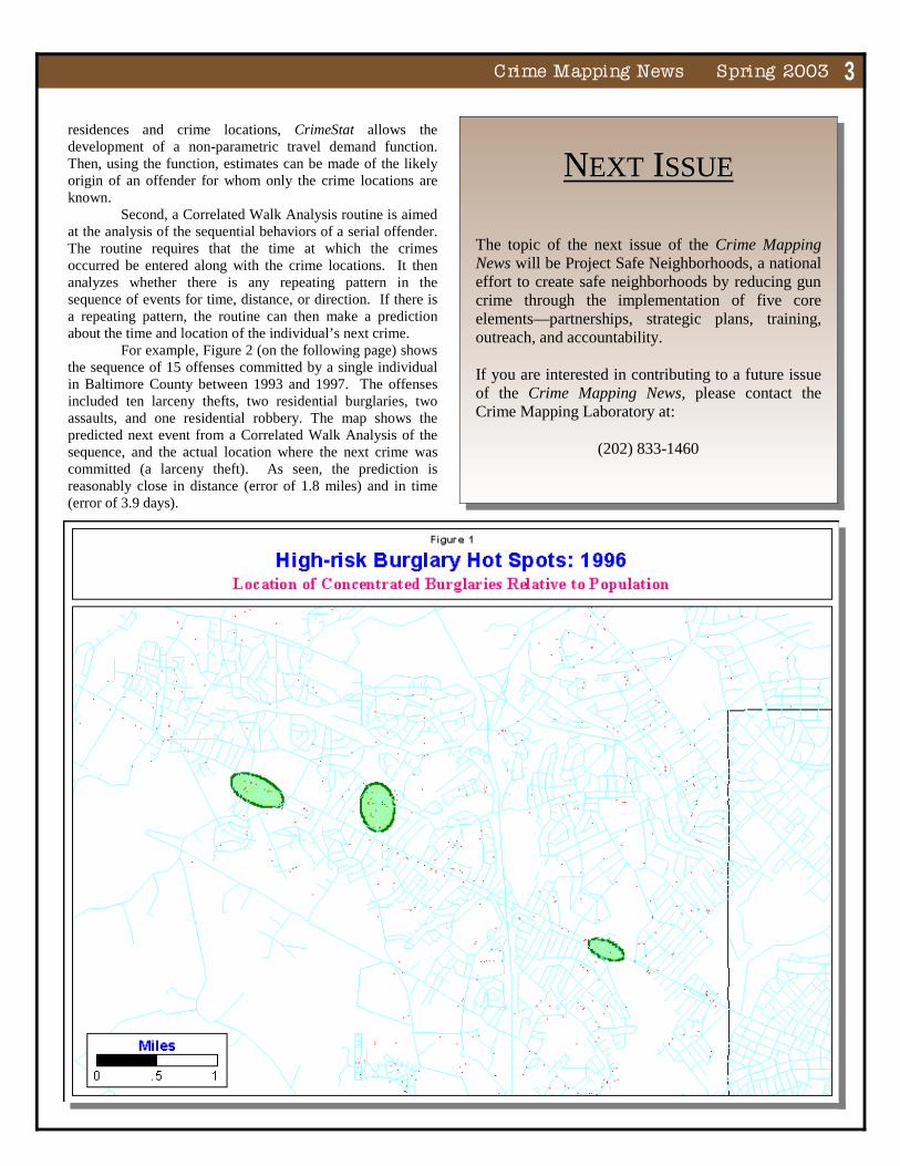
incidents. As an example, Figure 1 shows the standard deviational ellipses of first-order clusters of 1996 burglaries in Baltimore County, MD, relative to the 1990 population. The c l u s t e r s w e r e calculated with the risk-adjusted nearest neighbor clustering routine. As seen in

the map to the right, there are three hot spots where the number of burglaries is higher than that which would be expected on the basis of the population distribution. These are high risk burglary areas. Because the hot spot tools are complex algorithms, statistical significance must be tested with a Monte Carlo simulation. The nearest neighbor hierarchical clustering, the risk-adjusted nearest neighbor hierarchical clustering, and the STAC routines each have a Monte Carlo simulation that allows the estimation of approximate confidence intervals or test thresholds for these statistics. The Analysis of Serial Offenders There are two routines for analyzing the behavior of serial offenders. First, there is a Journey-to-Crime module. This is a method for estimating the likely residence location of a serial offender given the distribution of incidents and a model for travel distance. The routine requires data on the trip behavior of persons in order to estimate a travel demand function (e.g., the origins and destinations of offenders committing burglaries). Given a calibration sample of their

CrimeStat II (version 2.0 of the CrimeStat program) was recently released by the Mapping and Analysis for Public Safety program at the National Institute of Justice (NIJ). CrimeStat is a stand-alone spatial statistics program for the analysis of incident

locations. It was developed by Ned Levine & Associates under research grants from the National Institute of Justice. The National Institute of Justice is the sole distributor of CrimeStat and makes it available for free to law enforcement and criminal justice analysts and researchers.1

The program is Windows-based and interfaces with most desktop GIS programs. The purpose is to provide supplemental statistical tools to aid law enforcement agencies and criminal justice researchers in their crime mapping efforts. Version 2.0 is an evolutionary update of the program that involves improvements in functionality as well a s seve ra l ne w statistical functions. Interface with GIS Programs CrimeStat inputs incident locations (e.g., robbery locations) in .dbf, .shp, .dat, ASCII, and other formats. It can use spherical or projected coordinates. It can also treat zones as pseudo-points (or points with intensities). The program calculates various spatial statistics and writes graphical objects to ArcView®, ArcGis®, MapInfo®, Atlas GISTM, Surfer® for Windows, and ArcView Spatial Analyst©. Improvements in Version 2.0 Among the many improvements in functionality for Version 2.0 is the ability to read files that conform to the Open Database Connectivity (ODBC) standard, such as Microsoft Access or Excel, the ability to save and re-load program parameters, the ability to save and re-load alternative reference files, the output of Monte Carlo simulation data, and an improved help menu that is linked to the manual.

CrimeStat II by Ned Levine, PhD,

Ned Levine & Associates, Houston, TX

1 The program and documentation are available at http://www.icpsr.umich.edu/nacjd/crimestat.html.

“New statistics in Version 2.0 include the mode, the fuzzy mode, the STAC program (Spatial and Temporal Analysis of Crime) produced by the Illinois Criminal Justice Information Authority, a risk-adjusted nearest neighbor clustering routine, the Knox index, the Mantel index, and a Correlated Walk Analysis module.”

������������� �������������������3

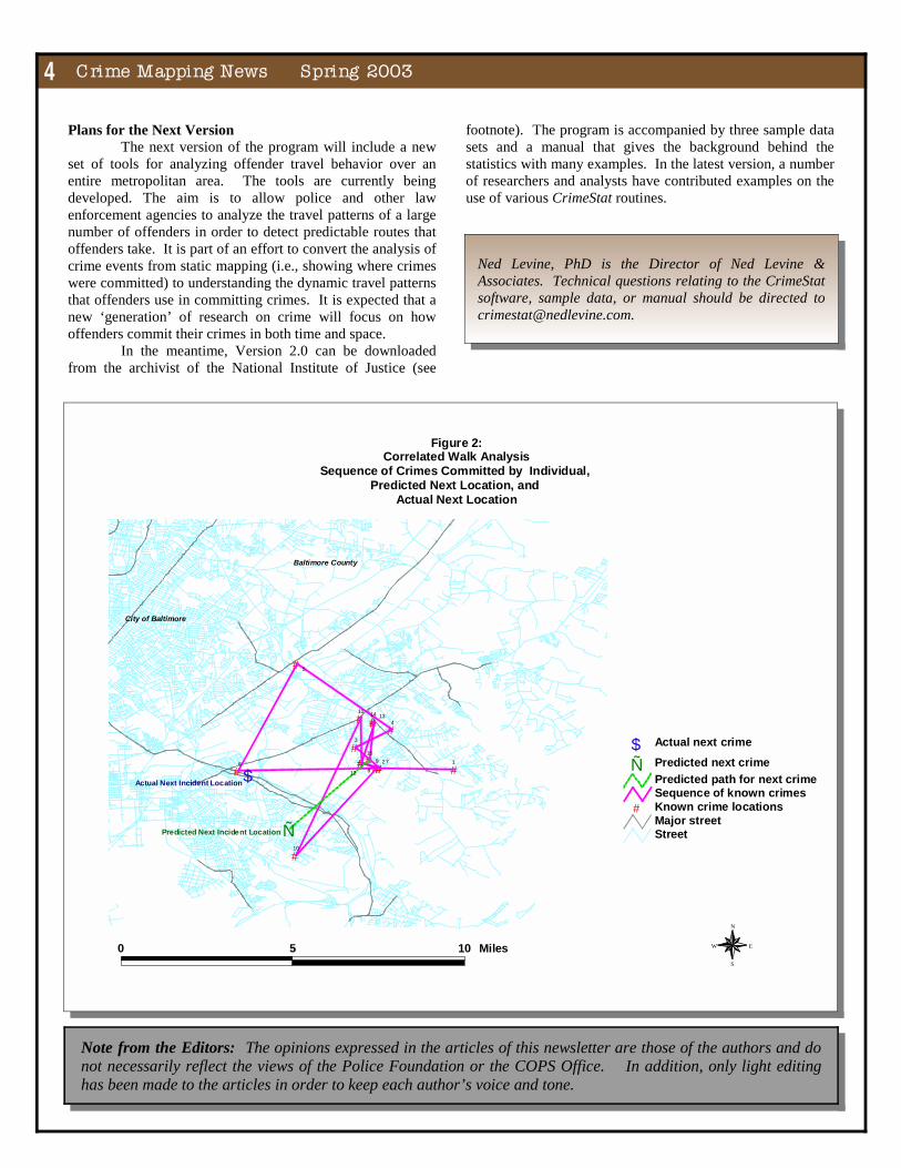
residences and crime locations, CrimeStat allows the development of a non-parametric travel demand function. Then, using the function, estimates can be made of the likely origin of an offender for whom only the crime locations are known. Second, a Correlated Walk Analysis routine is aimed at the analysis of the sequential behaviors of a serial offender. The routine requires that the time at which the crimes occurred be entered along with the crime locations. It then analyzes whether there is any repeating pattern in the sequence of events for time, distance, or direction. If there is a repeating pattern, the routine can then make a prediction about the time and location of the individual’s next crime. For example, Figure 2 (on the following page) shows the sequence of 15 offenses committed by a single individual in Baltimore County between 1993 and 1997. The offenses included ten larceny thefts, two residential burglaries, two assaults, and one residential robbery. The map shows the predicted next event from a Correlated Walk Analysis of the sequence, and the actual location where the next crime was committed (a larceny theft). As seen, the prediction is reasonably close in distance (error of 1.8 miles) and in time (error of 3.9 days).

NNNEXTEXTEXT I I ISSUESSUESSUE The topic of the next issue of the Crime Mapping News will be Project Safe Neighborhoods, a national effort to create safe neighborhoods by reducing gun crime through the implementation of five core elements—partnerships, strategic plans, training, outreach, and accountability. If you are interested in contributing to a future issue of the Crime Mapping News, please contact the Crime Mapping Laboratory at:

(202) 833-1460

�������������� ����������������4

footnote). The program is accompanied by three sample data sets and a manual that gives the background behind the statistics with many examples. In the latest version, a number of researchers and analysts have contributed examples on the use of various CrimeStat routines.

Plans for the Next Version The next version of the program will include a new set of tools for analyzing offender travel behavior over an entire metropolitan area. The tools are currently being developed. The aim is to allow police and other law enforcement agencies to analyze the travel patterns of a large number of offenders in order to detect predictable routes that offenders take. It is part of an effort to convert the analysis of crime events from static mapping (i.e., showing where crimes were committed) to understanding the dynamic travel patterns that offenders use in committing crimes. It is expected that a new ‘generation’ of research on crime will focus on how offenders commit their crimes in both time and space. In the meantime, Version 2.0 can be downloaded from the archivist of the National Institute of Justice (see

Ned Levine, PhD is the Director of Ned Levine & Associates. Technical questions relating to the CrimeStat software, sample data, or manual should be directed to crimestat@nedlevine.com.

Note from the Editors: The opinions expressed in the articles of this newsletter are those of the authors and do not necessarily reflect the views of the Police Foundation or the COPS Office. In addition, only light editing has been made to the articles in order to keep each author’s voice and tone.

##

#

#

#

# ## #

#

#

#

##

#

Ñ

$12

3

4

5

6 78

9

10

11

12

1314

15

Baltimore County

City of Baltimore

Predicted Next Incident Location

Actual Next Incident Location

StreetMajor street

# Known crime locationsSequence of known crimesPredicted path for next crime

Ñ Predicted next crime$ Actual next crime

0 5 10 Miles

N

EW

S

Figure 2:Correlated Walk Analysis

Sequence of Crimes Committed by Individual, Predicted Next Location, and

Actual Next Location

������������� �������������������5

Dr. Harold Shipman has become Britain’s most prolific serial killer. Between 1976 and 1998, he was responsible for killing 215 of his patients. For another 45, there is real suspicion of foul play. Shipman killed the majority of his victims with a lethal injection of diamorphine and hid the evidence by speedily processing his patients’ cremation certificates. To report on the scale of his crimes, the BBC prepared and screened a documentary on the day the Shipman Inquiry was published and used maps to help show the scale and impact of Shipman’s activities across the quiet Cheshire neighborhood of Hyde, England, where he was a general practitioner. The Shipman Public Inquiry In 1998, Shipman was charged and sentenced to life imprisonment for the murder of 15 of his patients. At the time, the British courts said that 15 cases were all they could h a n d l e fo r t h e prosecution, but after pressure by the families of some of S h i p m a n ’ s o t h e r supposed victims, a public inquiry was launched to investigate all 888 cases that were linked to Shipman. The Shipman Inquiry, led by High Court judge Dame Janet Smith, would investigate each case in turn and provide as complete an account as possible on Shipman’s criminality. This would include examining how many Shipman killed, the method he employed, and when the event occurred. To report on the impact of Shipman’s crimes, the BBC planned a documentary that would be screened on the day of the release of the Inquiry. Production began in the winter of 2001/2002, but with little certainty as to the exact date in the summer of 2002 when the Inquiry would be published. The documentary was mainly to involve interviews with families of Shipman’s victims, but included the idea of using maps to help represent the scale and volume of Shipman’s crimes in the town of Hyde. “We wanted both to give a powerful visual presentation of the extent of Shipman’s crimes over the course of his 24-year career as a family doctor and to show how he appeared to become more addicted to killing,” commented Kim Duke, the BBC editor and producer for the documentary. Kim’s vision was to use a series of maps and display Shipman’s crimes in a measles-like effect across Hyde—a point representing each crime, appearing in sequence in relation to the date when the death occurred. “The measles-like effect of an ever-increasing

number of cases appearing would illustrate how Shipman committed murder with increasing frequency until his arrest and also highlight clusters of cases.” With no mapping skills at her disposal, and with no idea how to source the map data she needed, Kim approached the Association for Geographic Information (AGI) and was directed to InfoTech’s crime mapping and analysis experience to help explore and realize the BBC’s vision. The Planning Phase Planning the maps for the documentary began in February 2002. The first challenge was to source name, address, and date of death information for each of the cases being investigated by the Inquiry. As this was a public inquiry, the information was published on the Inquiry’s Internet site (www.shipmaninquiry.com) after each case had been examined. Between the BBC and InfoTech, each case’s

details were entered into a single spread-sheet which was added to when new case material came to light. The second challenge was to source appropriate map data against which the case material was to be displayed. A number of samples of different

types of base mapping were explored, including Ordnance Survey’s MasterMap and raster products and TeleAtlas map data. “We were also keen to explore the use of aerial photographs as these would fit more powerfully within the documentary,” commented Mark Patrick, Senior Consultant at InfoTech. Using its contacts, InfoTech approached a number of aerial photography suppliers, sourced samples, and decided to use data from Getmapping. “We were delighted to provide InfoTech with aerial photography for this project,” said Rachel Eddy, Sales Director at Getmapping. “Aerial photography used to be specially commissioned, but now that we have national coverage, we could provide the exact area that InfoTech required with enough street-level detail to enable viewers to get a real understanding of how small the area was in which Shipman operated.” In early July, it was announced that the Shipman Inquiry would be published on Friday, July 19th. Aerial photographs were imported into MapInfo, and the spreadsheet of cases was completed as best as possible. The spreadsheet of case details could be completed, except for Dame Janet Smith’s verdicts on the remaining one-third of all cases. These would not be made public until the day the Inquiry was

Mapping Evil - The Impact of the Crimes of Dr. Harold Shipman by Spencer Chainey, Head of Consultancy Services

InfoTech Enterprises Europe

“To report on the impact of Shipman’s crimes, the BBC planned a documentary that would be screened on the day of the release of the Inquiry….The documentary was mainly to involve interviews with families of Shipman’s victims, but included the idea of using maps to help represent the scale and volume of Shipman’s crimes in the town of Hyde.”

�������������� ����������������6

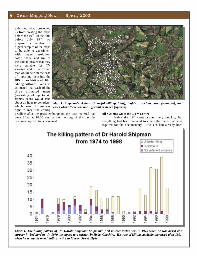
published which prevented us from creating the maps before the 19th. In the time before July 19th, we prepared a number of digital samples of the maps to be able to experiment with image resolution, color, shape, and size of the dots to ensure that they were suitable for TV viewing and in a format that would help in the ease of importing them into the BBC’s sophisticated film editing software. We also estimated that each of the three animated maps (consisting of up to 40 frames each) would take about an hour to complete, which meant that time was tight to meet the editing deadline after the press embargo on the case material had been lifted at 10:00 am on the morning of the day the documentary was to be screened.

All Systems Go at BBC TV Centre Friday the 19th came around very quickly, but everything had been prepared to create the maps that were required for the documentary. InfoTech had already been

Map 1. Shipman’s victims: Unlawful killings (dots), highly suspicious cases (triangles), and cases where there was not sufficient evidence (squares).

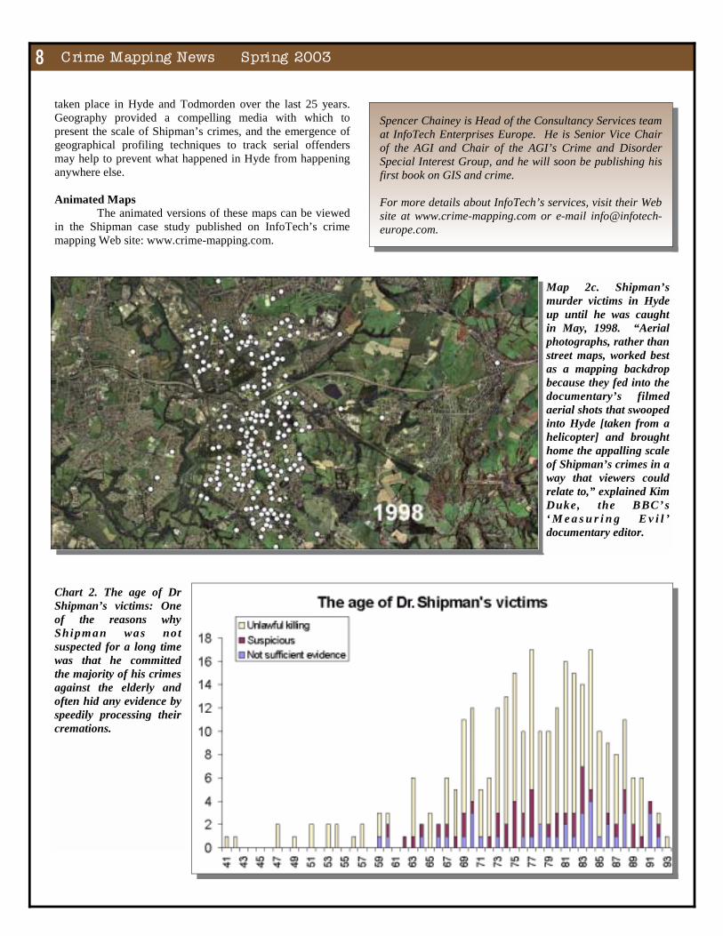
Chart 1. The killing pattern of Dr. Harold Shipman: Shipman’s first murder victim was in 1978 when he was based at a surgery in Todmorden. In 1979, he moved to a surgery in Hyde, Cheshire. His rate of killing suddenly increased after 1991, when he set up his own family practice in Market Street, Hyde.

������������� �������������������7

given a preview of the documentary that contained the majority of the required interview footage (minus the voiceover), and blank spaces where the maps were to fit in. Camped in an editing suite at BBC TV Centre, London, with Kim and the picture editor, Mark Patrick and I set to work as soon as the office’s fax machine began receiving the confirmed case details that were being sent by BBC Manchester after the 10:00 am press embargo had been lifted. “The case material was shooting down the fax at the same time we could see the news being reported live from Manchester on BBC 24,” said Mark Patrick. The immediate headline was that Shipman had actually killed over 30 people more than the 180 for which he had been initially suspected. With the case information loaded in, updated, and geocoded, the three animated maps could be produced. Sue Johnston (a famous British actress who has played a number of BBC roles, most recently the role of a criminal psychological profiler in the TV series ‘Waking the Dead’) joined the team to provide the voiceover for the docu-mentary. Documentary Maps The first animated map that was to appear within the first two minutes o f t h e 6 0 - m i n u t e documentary showed all 215 people Shipman had killed and those that were highly suspicious or where there was insufficient evidence to say whether he had killed the person or not (Map 1). “Immediately you could see how Shipman had appeared to become addicted to killing. His killing rate tended to increase year by year from 1976 to 1990, then all went quiet until he moved surgeries and set up his own private practice in 1991. From that point forward until he was caught in May 1998, the scale of what he was doing was quite staggering,” said Mark Patrick. The second map (Maps 2a, 2b, and 2c) brought this home further

when a time clock was added to the image to show just those cases that had been confirmed as ‘unlawful killing.’ The final animated map (Map 3 on the following page) showed the full extent of Shipman’s crimes and work that was required by Dame Janet Smith and the Public Inquiry in investigating all cases. The map also showed the full extent of just how much this family doctor had destroyed a community. Producing the maps for the documentary was a very sobering experience. Mapping data can often sanitize GIS professionals to the detail that lies behind each symbol. The fact that each dot represented a person’s life left you feeling very touched, appalled, and connected to the events that had

Map 2a. Shipman’s murder victims in Hyde up until 1980.

Map 2b. Shipman’s murder victims in Hyde up until 1990.

�������������� ����������������8

taken place in Hyde and Todmorden over the last 25 years. Geography provided a compelling media with which to present the scale of Shipman’s crimes, and the emergence of geographical profiling techniques to track serial offenders may help to prevent what happened in Hyde from happening anywhere else. Animated Maps The animated versions of these maps can be viewed in the Shipman case study published on InfoTech’s crime mapping Web site: www.crime-mapping.com.

Spencer Chainey is Head of the Consultancy Services team at InfoTech Enterprises Europe. He is Senior Vice Chair of the AGI and Chair of the AGI’s Crime and Disorder Special Interest Group, and he will soon be publishing his first book on GIS and crime. For more details about InfoTech’s services, visit their Web site at www.crime-mapping.com or e-mail info@infotech-europe.com.

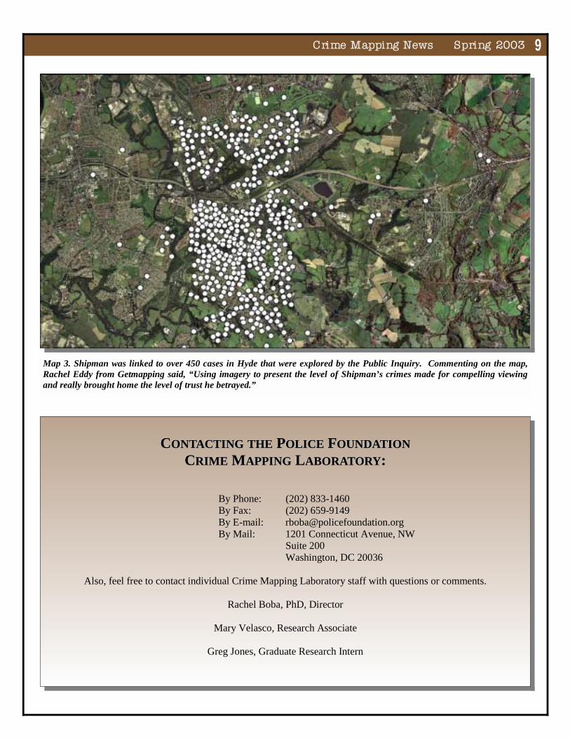
Map 2c. Shipman’s murder victims in Hyde up until he was caught in May, 1998. “Aerial photographs, rather than street maps, worked best as a mapping backdrop because they fed into the documentary’s filmed aerial shots that swooped into Hyde [taken from a helicopter] and brought home the appalling scale of Shipman’s crimes in a way that viewers could relate to,” explained Kim Duke, the BBC’s ‘ M e a s u r i n g E v i l ’ documentary editor.

Chart 2. The age of Dr Shipman’s victims: One of the reasons why Shipm an was no t suspected for a long time was that he committed the majority of his crimes against the elderly and often hid any evidence by speedily processing their cremations.

������������� �������������������9

CCCONTACTINGONTACTINGONTACTING THETHETHE P P POLICEOLICEOLICE F F FOUNDATIONOUNDATIONOUNDATION CCCRIMERIMERIME M M MAPPINGAPPINGAPPING L L LABORATORYABORATORYABORATORY:::

By Phone: (202) 833-1460 By Fax: (202) 659-9149 By E-mail: rboba@policefoundation.org By Mail: 1201 Connecticut Avenue, NW Suite 200 Washington, DC 20036

Also, feel free to contact individual Crime Mapping Laboratory staff with questions or comments.

Rachel Boba, PhD, Director

Mary Velasco, Research Associate

Greg Jones, Graduate Research Intern

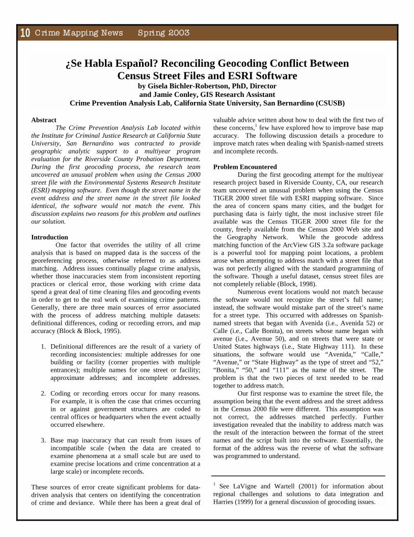
Map 3. Shipman was linked to over 450 cases in Hyde that were explored by the Public Inquiry. Commenting on the map, Rachel Eddy from Getmapping said, “Using imagery to present the level of Shipman’s crimes made for compelling viewing and really brought home the level of trust he betrayed.”

�������������� ����������������10

valuable advice written about how to deal with the first two of these concerns,1 few have explored how to improve base map accuracy. The following discussion details a procedure to improve match rates when dealing with Spanish-named streets and incomplete records. Problem Encountered

During the first geocoding attempt for the multiyear research project based in Riverside County, CA, our research team uncovered an unusual problem when using the Census TIGER 2000 street file with ESRI mapping software. Since the area of concern spans many cities, and the budget for purchasing data is fairly tight, the most inclusive street file available was the Census TIGER 2000 street file for the county, freely available from the Census 2000 Web site and the Geography Network. While the geocode address matching function of the ArcView GIS 3.2a software package is a powerful tool for mapping point locations, a problem arose when attempting to address match with a street file that was not perfectly aligned with the standard programming of the software. Though a useful dataset, census street files are not completely reliable (Block, 1998). Numerous event locations would not match because the software would not recognize the street’s full name; instead, the software would mistake part of the street’s name for a street type. This occurred with addresses on Spanish-named streets that began with Avenida (i.e., Avenida 52) or Calle (i.e., Calle Bonita), on streets whose name began with avenue (i.e., Avenue 50), and on streets that were state or United States highways (i.e., State Highway 111). In these situations, the software would use “Avenida,” “Calle,” “Avenue,” or “State Highway” as the type of street and “52,” “Bonita,” “50,” and “111” as the name of the street. The problem is that the two pieces of text needed to be read together to address match.

Our first response was to examine the street file, the assumption being that the event address and the street address in the Census 2000 file were different. This assumption was not correct, the addresses matched perfectly. Further investigation revealed that the inability to address match was the result of the interaction between the format of the street names and the script built into the software. Essentially, the format of the address was the reverse of what the software was programmed to understand.

Abstract The Crime Prevention Analysis Lab located within the Institute for Criminal Justice Research at California State University, San Bernardino was contracted to provide geographic analytic support to a multiyear program evaluation for the Riverside County Probation Department. During the first geocoding process, the research team uncovered an unusual problem when using the Census 2000 street file with the Environmental Systems Research Institute (ESRI) mapping software. Even though the street name in the event address and the street name in the street file looked identical, the software would not match the event. This discussion explains two reasons for this problem and outlines our solution. Introduction One factor that overrides the utility of all crime analysis that is based on mapped data is the success of the georeferencing process, otherwise referred to as address matching. Address issues continually plague crime analysis, whether those inaccuracies stem from inconsistent reporting practices or clerical error, those working with crime data spend a great deal of time cleaning files and geocoding events in order to get to the real work of examining crime patterns. Generally, there are three main sources of error associated with the process of address matching multiple datasets: definitional differences, coding or recording errors, and map accuracy (Block & Block, 1995).

1. Definitional differences are the result of a variety of recording inconsistencies: multiple addresses for one building or facility (corner properties with multiple entrances); multiple names for one street or facility; approximate addresses; and incomplete addresses.

2. Coding or recording errors occur for many reasons. For example, it is often the case that crimes occurring in or against government structures are coded to central offices or headquarters when the event actually occurred elsewhere.

3. Base map inaccuracy that can result from issues of

incompatible scale (when the data are created to examine phenomena at a small scale but are used to examine precise locations and crime concentration at a large scale) or incomplete records.

These sources of error create significant problems for data-driven analysis that centers on identifying the concentration of crime and deviance. While there has been a great deal of

¿Se Habla Español? Reconciling Geocoding Conflict Between Census Street Files and ESRI Software

by Gisela Bichler-Robertson, PhD, Director and Jamie Conley, GIS Research Assistant

Crime Prevention Analysis Lab, California State University, San Bernardino (CSUSB)

1 See LaVigne and Wartell (2001) for information about regional challenges and solutions to data integration and Harries (1999) for a general discussion of geocoding issues.

������������� �������������������11

box and nothing was typed into the “Replace With” dialog space, then “Replace All” was chosen. This process was repeated until all of the troublesome streets were dealt with. The final result was a street file with three columns—Pretype with street type data only for the problem streets, Name with the actual street name, and the original street name column.3

Finally, the DBF file was re-sorted by street segment identification number (the first column of the street file) so that the file was in its original order. Changes were saved (as a DBF file). This cleaning process was repeated for each of the DBF tables (recall that the county file was split into three regions). Using the Geoprocessing Extension of ArcView 3.2a, the three separate street files were merged into a single file again. This step would not be necessary if the original

DBF table were cleaned in its original form. Step Two: Instructing the Software Once the street file was adjusted, the geocoding software had to be told what to look for in the Census 2000 street file. When address matching in ArcView GIS 3.2a, a geocoding index must

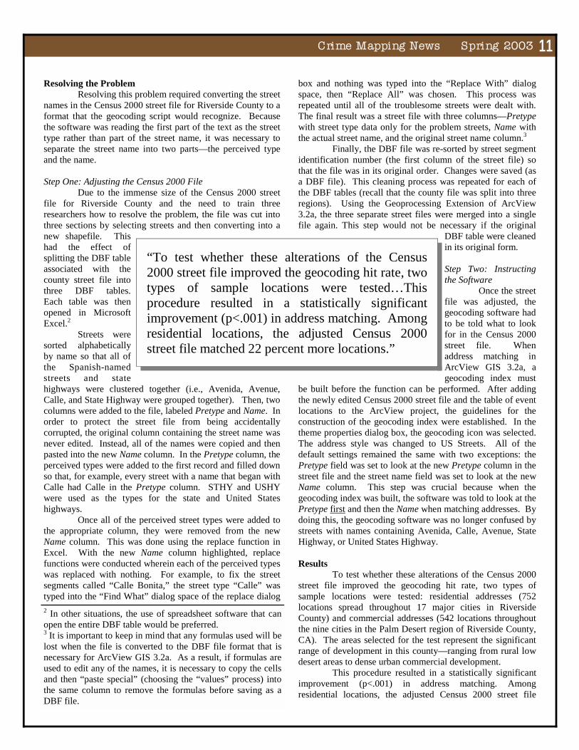
be built before the function can be performed. After adding the newly edited Census 2000 street file and the table of event locations to the ArcView project, the guidelines for the construction of the geocoding index were established. In the theme properties dialog box, the geocoding icon was selected. The address style was changed to US Streets. All of the default settings remained the same with two exceptions: the Pretype field was set to look at the new Pretype column in the street file and the street name field was set to look at the new Name column. This step was crucial because when the geocoding index was built, the software was told to look at the Pretype first and then the Name when matching addresses. By doing this, the geocoding software was no longer confused by streets with names containing Avenida, Calle, Avenue, State Highway, or United States Highway. Results To test whether these alterations of the Census 2000 street file improved the geocoding hit rate, two types of sample locations were tested: residential addresses (752 locations spread throughout 17 major cities in Riverside County) and commercial addresses (542 locations throughout the nine cities in the Palm Desert region of Riverside County, CA). The areas selected for the test represent the significant range of development in this county—ranging from rural low desert areas to dense urban commercial development. This procedure resulted in a statistically significant improvement (p<.001) in address matching. Among residential locations, the adjusted Census 2000 street file

Resolving the Problem Resolving this problem required converting the street

names in the Census 2000 street file for Riverside County to a format that the geocoding script would recognize. Because the software was reading the first part of the text as the street type rather than part of the street name, it was necessary to separate the street name into two parts—the perceived type and the name. Step One: Adjusting the Census 2000 File Due to the immense size of the Census 2000 street file for Riverside County and the need to train three researchers how to resolve the problem, the file was cut into three sections by selecting streets and then converting into a new shapefile. This had the effect of splitting the DBF table associated with the county street file into three DBF tables. Each table was then opened in Microsoft Excel.2 Streets were sorted alphabetically by name so that all of the Spanish-named streets and state highways were clustered together (i.e., Avenida, Avenue, Calle, and State Highway were grouped together). Then, two columns were added to the file, labeled Pretype and Name. In order to protect the street file from being accidentally corrupted, the original column containing the street name was never edited. Instead, all of the names were copied and then pasted into the new Name column. In the Pretype column, the perceived types were added to the first record and filled down so that, for example, every street with a name that began with Calle had Calle in the Pretype column. STHY and USHY were used as the types for the state and United States highways.

Once all of the perceived street types were added to the appropriate column, they were removed from the new Name column. This was done using the replace function in Excel. With the new Name column highlighted, replace functions were conducted wherein each of the perceived types was replaced with nothing. For example, to fix the street segments called “Calle Bonita,” the street type “Calle” was typed into the “Find What” dialog space of the replace dialog 2 In other situations, the use of spreadsheet software that can open the entire DBF table would be preferred. 3 It is important to keep in mind that any formulas used will be lost when the file is converted to the DBF file format that is necessary for ArcView GIS 3.2a. As a result, if formulas are used to edit any of the names, it is necessary to copy the cells and then “paste special” (choosing the “values” process) into the same column to remove the formulas before saving as a DBF file.

“To test whether these alterations of the Census 2000 street file improved the geocoding hit rate, two types of sample locations were tested…This procedure resulted in a statistically significant improvement (p<.001) in address matching. Among residential locations, the adjusted Census 2000 street file matched 22 percent more locations.”

�������������� ����������������12

matched 22 percent more locations (see Table 1). Clearly, this procedure dealt with a naming tendency that affected a substantial number of streets in the region. Though significant, the change for commercial properties was not as dramatic—this geocoding rate improved by nine percent. However, among different types of properties, the improvement was remarkable. Revisiting the Geocoding Hit Rate

The inability to achieve 100 percent matching on all files led the research team to revisit the geocoding hit rate problem. By doing interactive re-matching, it was discovered that the remaining addresses were not matching because the numeric address ranges were missing from the base street file and, in some cases, even the name of the street was absent. Breadth of the Issue

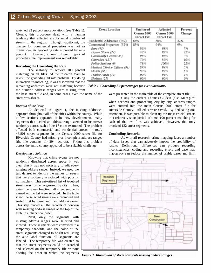
As depicted in Figure 1, the missing addresses appeared throughout all of the cities within the county. While a few sections appeared to be new developments, many segments that lacked an address range seemed to be strewn randomly across each of the 17 cities examined. The problem affected both commercial and residential streets: in total, 43,801 street segments in the Census 2000 street file for Riverside County had missing or incomplete address ranges (the file contains 114,294 records). Fixing this problem across the entire county appeared to be a sizable challenge. Developing a Solution Knowing that crime events are not randomly distributed across space, it was clear that it was not necessary to edit every missing address range. Instead, we used the test dataset to identify the names of streets that were routinely associated with poor or no matches. This prioritized list of troubled streets was further organized by city. Then, using the query function, all street segments named on the list were selected. In the table view, the selected streets were promoted and sorted first by name and then address range. This step placed all the records of concern with missing address ranges at the top of the table in alphabetical order.

Next, only the segments with missing address ranges were selected and viewed. These segments were converted to a temporary shapefile, and the color of the street segments changed to bright red. Using the auto label function, all segments are labeled. The temporary file was created so that the street segments could be searched and selected on the temporary file without altering the order in which the segments

were presented in the main table of the complete street file. Using the current Thomas Guide® (also MapQuest when needed) and proceeding city by city, address ranges were entered into the main Census 2000 street file for Riverside County. All edits were saved. By dedicating one afternoon, it was possible to clean up the most crucial streets in a relatively short period of time; 100 percent matching for each of the test files was achieved. However, this only involved 122 street segments. Concluding Remarks

As with all research, crime mapping faces a number of data issues that can adversely impact the credibility of results. Definitional differences can produce recording inconsistencies, coding and recording errors and base map inaccuracy can reduce the number of usable cases and limit

Table 1. Geocoding hit percentages for event locations.

Figure 1. Illustration of street segments missing address ranges.

������������� �������������������13

the utility of analysis. This discussion presented two strategies to resolve a kink that developed between Census street files and ESRI software. While the problem was encountered when using ArcView 3.2a, the problem remained when we switched to ArcGIS. Essentially, the software was unable to address match events occurring on Spanish-named streets. This is a disconcerting issue for agencies located in the southwest region of the United States.

Addressing the issue of Spanish-named streets had a remarkable impact on the geocoding rate; however, a considerable number of unmatchable events remained. The second issue relating to missing address ranges remains a significant concern, plaguing all users of Census data.

Clearly, by cleaning against such a small test data set, a great deal of inaccuracy remains in the base map. Repeating the process to clean street ranges with different datasets will lead to continued, albeit sluggish improvements in geocoding hit rates. However, with each repetition of this cleaning process, a greater number of cases will map. Running this procedure with a single crime type or for a specific beat each time may improve the efficiency of the procedure. The time and effort invested in developing a more accurate base map will be realized in the quality of analysis produced. Raising the hit rate closer to 100 percent will improve the utility of crime mapping and may lead to more effective problem diagnosis. References Block, R.L. & C.R. Block. (1995). “Space, place and crime:

Hot spot areas and hot places of liquor-related crime.” In R.V. Clarke (Series Ed.), J.E. Eck & D. Weisburd (Vol. Eds.), Crime and place: Crime prevention studies Vol. 4. (pp. 145-184). New York: Criminal Justice Press.

Block, C.R. (1998). “The GeoArchive: An information

foundation for community policing.” In R.V. Clarke (Series Ed.), D. Weisburd & T. McEwen, (Vol. Eds.), Crime mapping and crime prevention: Crime prevention studies Vol. 8. (pp. 27-81). New York: Criminal Justice Press.

Harries, K. (1999). Mapping crime: Principle and practice.

Washington, DC: National Institute of Justice. LaVigne, N. & J. Wartell. (2001). Mapping across

boundaries: Regional crime analysis. Washington, DC: Police Executive Research Forum.

Gisela Bichler-Robertson, PhD is the Director of the Crime Prevention Analysis Lab at California State University, San Bernardino. She can be contacted via e-mail at gbichler@csusb.edu. Jamie Conley is a GIS Research Assistant at the Crime Prevention Analysis Lab and can be contacted via e-mail at jeconley@juno.com.

FFFURTHERURTHERURTHER D D DISCUSSIONISCUSSIONISCUSSION::: “C“C“CRIMERIMERIME A A ANALYSISNALYSISNALYSIS C C CHALLENGEHALLENGEHALLENGE”””

In Volume 4 of the Crime Mapping News, we presented the “Crime Analysis Challenge,” composed of nine questions designed to stimulate thought and discussion among the crime analysis and mapping community. We received a comment from a law enforcement practitioner that requires a follow-up explanation. The comment (paraphrased below) pertains to Question 6, concerning the prediction of future events in a crime series. (For the complete question and answer, please see Volume 4, Issue 3 of the Crime Mapping News, available on both the Police Foundation and COPS Office Web sites). The comment (paraphrased): I think there is a mistake with the answer for Question 6 of the Crime Analysis Challenge. You are stating that within the one standard deviation rectangle, there is a 0.68 probability. Yet using the same reasoning, you are using the joint probability (of independent events) and assuming that the X and Y probabilities are independent, the probability would be 0.46 (0.68 x 0.68). The same holds for a standard deviation ellipse (0.46). Of course, we are assuming that there is a normal distribution of points at each axis. Response: The standard distance, the geographic equivalent of the standard deviation (equal to the square root of the mean squared distance of a point from the spatial mean), encompasses approximately 68% of the points in a distribution. However, the standard deviational rectangle does not seem to appear in the quantitative geography or spatial analysis literature. It is used in crime analysis, but the only definition we could locate with an equation was in Gottlieb, S., Arenberg, S., & Singh, R. (1998), Crime analysis: From first report to final arrest. On page 452, it states, “This rectangle now represents the geographic area in which 68% of the crimes (one standard deviation) have occurred.” But according to the suggested method of calculation outlined on pages 449-452, X and Y values are treated independently, resulting in such a rectangle encompassing only 46% of the incidents (0.68 x 0.68). If Gottlieb et al.’s method were followed, the forecasting probability would have to be reduced (by a factor of 0.68) and would have been 0.46. But in the map shown in the Crime Analysis Challenge for Question 6, we used a true standard deviational rectangle (or approximation thereof) that encompassed 3 of the 5 crimes. We therefore used 0.68 as the probability factor. However, to be exact, we should have used 3/5 or 0.60 in which case the resulting answer would have been a 21% to 24% chance and not 24% to 27%.

�������������� ����������������14

Upcoming Conferences and Training

Early Reminders! Environmental Systems Research Institute (ESRI) International User Conference July 7-11, 2003 San Diego, CA www.esri.com Annual Conference on Criminal Justice Research and Evaluation July 28-30, 2003 Washington, DC http://nijpcs.org Crime Mapping & Analysis Program (CMAP): ArcView Class July 28-August 1, 2003 NCTC, PA Contact: Danelle Digiosio, ddigiosi@du.edu or (800) 416-8086

General Web Resources for Training Seminars

and Conferences http://www.urisa.org/meetings.htm http://www.ifp.uni-stuttgart.de/ifp/gis/ conferences.html http://www.geoinfosystems.com/calendar.htm http://msdis.missouri.edu/ http://magicweb.kgs.ukans.edu/magic/ magic_net.html http://www.nsgic.org/ http://www.mapinfo.com/events http://www.esri.com/events http://www.ojp.usdoj.gov/cmrc/training/ welcome.html http://www.nlectc.org/nlectcrm/ http://www.nijpcs.org/upcoming.htm http://www.usdoj.gov/cops/gpa/tta/default.htm http://giscenter.isu.edu/training/training.htm http://www.alphagroupcenter.com/index2.htm http://www.cicp.org http://www.actnowinc.org http://www.ialeia.org

April

Rio Hondo GIS/GPS Public Safety Training Center: ArcView Training April 21-25, 2003 Whittier, CA Contact: Bob Feliciano, bfeliciano@riohondo.edu or (562) 692-0921

May International Association of Chiefs of Police (IACP): Introduction to Crime Analysis May 7-9, 2003 Oswego, NY Contact: Shirley Mackey, mackeys@theiacp.org International Association of Chiefs of Police (IACP): Advanced Crime Analysis May 12-14, 2003 Oswego, NY Contact: Shirley Mackey, mackeys@theiacp.org Crime Mapping & Analysis Program (CMAP): ArcView Class May 19-23, 2003 Northeast Counterdrug Training Center (NCTC), PA Contact: Danelle Digiosio, ddigiosi@du.edu or (800) 416-8086 International Association of Law Enforcement Intelligence Analysts (IALEIA) 2003 Annual Conference May 25-30, 2003 Boston, MA www.ialeia.org

June Massachusetts Association of Crime Analysts (MACA) 2003 Annual Training Conference June 9-12, 2003 Hyannis, MA www.macrimeanalysts.com

������������� �������������������15

ABOUT THE POLICE FOUNDATIONABOUT THE POLICE FOUNDATIONABOUT THE POLICE FOUNDATIONABOUT THE POLICE FOUNDATION

OFFICE OF RESEARCHOFFICE OF RESEARCHOFFICE OF RESEARCHOFFICE OF RESEARCH

D. Kim Rossmo, PhD Director of Research

Rachel Boba, PhD Director, Crime Mapping Laboratory

David Weisburd, PhD Senior Fellow

Mary Velasco, BS Research Associate

Vanessa Ruvalcaba, BA Research Assistant

Greg Jones, MA Graduate Research Intern

Tamika McDowell, BA Senior Administrative Assistant

BOARD OF DIRECTORSBOARD OF DIRECTORSBOARD OF DIRECTORSBOARD OF DIRECTORS

Chairman William G. Milliken

President

Hubert Williams

David Cole

Wade Henderson

William H. Hudnut III

W. Walter Menninger

Laurie O. Robinson

Henry Ruth

Weldon J. Rougeau

Alfred A. Slocum

Maria Vizcarrondo-DeSoto

Kathryn J. Whitmire

1201 Connecticut Avenue, NW, Suite 200, Washington, DC 20036 (202) 833-1460 !!!! Fax (202) 659-9149 !!!! e-mail: pfinfo@policefoundation.org

www.policefoundation.org

This project was supported by cooperative agreement #2002-CK-WX-0303 awarded by the Office of Community Oriented Policing Services, US Department of Justice. Points of view or opinions contained in this document are those of the authors and do not necessarily represent the official position or policies of the US Department of Justice.

The Police Foundation is a private, independent, not-for-profit organization dedicated to supporting innovation and improvement in policing through its research, technical assistance, and communications programs. Established in 1970, the foundation has conducted seminal research in police behavior, policy, and procedure, and works to transfer to local agencies the best new information about practices for dealing effectively with a range of important police operational and administrative concerns. Motivating all of the foundation’s efforts is the goal of efficient, humane policing that operates within the framework of democratic principles and the highest ideals of the nation.