Embed Size (px)
Citation preview

The College of Wooster LibrariesOpen Works
Senior Independent Study Theses
2018
Crime Around the World: Using MathematicalModeling Techniques to Model AggregatedWorldwide Crime RatesKelly M. SteurerThe College of Wooster, [email protected]
Follow this and additional works at: https://openworks.wooster.edu/independentstudy
This Senior Independent Study Thesis Exemplar is brought to you by Open Works, a service of The College of Wooster Libraries. It has been acceptedfor inclusion in Senior Independent Study Theses by an authorized administrator of Open Works. For more information, please [email protected].
© Copyright 2018 Kelly M. Steurer
Recommended CitationSteurer, Kelly M., "Crime Around the World: Using Mathematical Modeling Techniques to Model Aggregated Worldwide CrimeRates" (2018). Senior Independent Study Theses. Paper 8287.https://openworks.wooster.edu/independentstudy/8287

Crime Around theWorld:using mathematicalmodeling techniques tomodel aggregated
worldwide crime rates
Independent Study Thesis
Presented in Partial Fulfillment of theRequirements for the Degree Bachelor of Arts inthe Department of Mathematics and Computer
Science at The College of Wooster
byKelly Steurer
The College of Wooster2018
Advised by:
Dr. Drew Pasteur


Abstract
This aim of this study was to determine what affects aggregate crime rates
around the world. This thesis used Mathematical Modeling techniques to
build generalized linear models for homicide rates and burglary and
housebreaking rates using the following predictive factors: economic
indicators, education rates, government quality indicators, ethno-linguistic
fractionalization, GDP per capita and its growth, drug consumption rates, and
age and gender ratios. We used a series of factor selection techniques
including linear and stepwise regressions, principal component analysis, and
regression analysis to select factors to use to build final models of homicide
and burglary and housebreaking.
iii


Acknowledgements
I would like to thank my advisor, Dr. Pasteur, for giving me the help and
encouragement throughout the year that I needed to complete this project. I
would also like to thank my mom and dad for providing me with the
opportunity to enrich my education by attending the College of Wooster.
Without their love and support, I would not have been able to make it this far.
Finally, I would like to thank each and every one of my friends for putting up
with me this year, as the stress of this thesis made my presence quite
unpleasant at times.
v


Contents
Abstract iii
Acknowledgements v
1 Introduction 1
1.1 Poverty and Income Inequality . . . . . . . . . . . . . . . . . . . . 1
1.1.1 Poverty . . . . . . . . . . . . . . . . . . . . . . . . . . . . . . 2
1.1.2 Income Inequality . . . . . . . . . . . . . . . . . . . . . . . 3
1.2 Education . . . . . . . . . . . . . . . . . . . . . . . . . . . . . . . . 6
1.3 Government Quality . . . . . . . . . . . . . . . . . . . . . . . . . . 7
1.4 Ethno-Linguistic Fractionalization . . . . . . . . . . . . . . . . . . 10
1.5 Latin America and the Caribbean . . . . . . . . . . . . . . . . . . . 13
1.6 Other Factors . . . . . . . . . . . . . . . . . . . . . . . . . . . . . . 15
1.6.1 GDP Per Capita . . . . . . . . . . . . . . . . . . . . . . . . . 15
1.6.2 Drug Consumption . . . . . . . . . . . . . . . . . . . . . . . 16
1.6.3 Age . . . . . . . . . . . . . . . . . . . . . . . . . . . . . . . . 17
1.6.4 Gender . . . . . . . . . . . . . . . . . . . . . . . . . . . . . . 18
vii

viii CONTENTS
2 Methodology 19
2.1 Data Standardization . . . . . . . . . . . . . . . . . . . . . . . . . . 19
2.2 Linear Regressions . . . . . . . . . . . . . . . . . . . . . . . . . . . 21
2.3 Stepwise Regressions . . . . . . . . . . . . . . . . . . . . . . . . . . 22
2.3.1 T-test . . . . . . . . . . . . . . . . . . . . . . . . . . . . . . . 22
2.3.2 Overfitting . . . . . . . . . . . . . . . . . . . . . . . . . . . . 23
2.3.3 Stepwise Regression . . . . . . . . . . . . . . . . . . . . . . 25
2.4 Eigenvalues and Eigenvectors . . . . . . . . . . . . . . . . . . . . . 26
2.5 Principal Component Analysis . . . . . . . . . . . . . . . . . . . . 27
2.5.1 Covariance Matrices . . . . . . . . . . . . . . . . . . . . . . 28
2.5.2 New Predictors . . . . . . . . . . . . . . . . . . . . . . . . . 29
2.6 Normal Distributions . . . . . . . . . . . . . . . . . . . . . . . . . . 30
2.7 Residual Analysis . . . . . . . . . . . . . . . . . . . . . . . . . . . . 31
2.8 Machine Learning . . . . . . . . . . . . . . . . . . . . . . . . . . . . 34
2.8.1 Decision Trees . . . . . . . . . . . . . . . . . . . . . . . . . . 34
2.8.2 Regression Trees . . . . . . . . . . . . . . . . . . . . . . . . 36
2.8.3 Random Forests . . . . . . . . . . . . . . . . . . . . . . . . . 37
2.9 Generalized Linear Models . . . . . . . . . . . . . . . . . . . . . . 38
3 Results 41
3.1 Data Sources . . . . . . . . . . . . . . . . . . . . . . . . . . . . . . . 41
3.1.1 Assumptions . . . . . . . . . . . . . . . . . . . . . . . . . . 45
3.2 Linear Regressions . . . . . . . . . . . . . . . . . . . . . . . . . . . 46
3.2.1 Homicide Slopes . . . . . . . . . . . . . . . . . . . . . . . . 47
3.2.2 Burglary and Housebreaking Slopes . . . . . . . . . . . . . 48

3.3 Residual Analysis . . . . . . . . . . . . . . . . . . . . . . . . . . . . 50
3.3.1 Residual Plots with Homicide Rates . . . . . . . . . . . . . 51
3.3.2 Residual Plots with Burglary and Housebreaking Rates . . 53
3.4 Principal Component Analysis . . . . . . . . . . . . . . . . . . . . 54
3.5 Trends in Individual Regions . . . . . . . . . . . . . . . . . . . . . 57
3.5.1 Worldwide Averages . . . . . . . . . . . . . . . . . . . . . . 58
3.5.2 Regional Trends . . . . . . . . . . . . . . . . . . . . . . . . . 58
3.5.3 Trends in Developing and Developed Countries . . . . . . 63
3.6 Stepwise Regressions . . . . . . . . . . . . . . . . . . . . . . . . . . 66
3.7 Final Models . . . . . . . . . . . . . . . . . . . . . . . . . . . . . . . 68
3.7.1 Homicide Model . . . . . . . . . . . . . . . . . . . . . . . . 70
3.7.2 Burglary and Housebreaking Model . . . . . . . . . . . . . 71
4 Discussion 73
4.1 Modeling Results . . . . . . . . . . . . . . . . . . . . . . . . . . . . 73
4.1.1 Homicide Model . . . . . . . . . . . . . . . . . . . . . . . . 74
4.1.2 Burglary and Housebreaking Model . . . . . . . . . . . . . 75
4.2 Link Between Property Crime and Homicide . . . . . . . . . . . . 76
4.2.1 Burglary and Housebreaking Data Irregularities . . . . . . 77
4.3 Flaws in the Final Models . . . . . . . . . . . . . . . . . . . . . . . 81
4.4 Future Work . . . . . . . . . . . . . . . . . . . . . . . . . . . . . . . 82
A Tables and Lists 85


List of Figures
1.1 The Lorenz curve with the Line of Equality . . . . . . . . . . . . . 4
1.2 Percentage of homicides committed by various age groups . . . . 17
2.1 Illustration of a normal distribution . . . . . . . . . . . . . . . . . 30
2.2 Residual plot with a random distribution . . . . . . . . . . . . . . 32
2.3 Residual plot with an unbalanced y-axis . . . . . . . . . . . . . . . 32
2.4 Residual plot with an unbalanced x-axis . . . . . . . . . . . . . . . 33
2.5 Binary decision tree with terminology . . . . . . . . . . . . . . . . 35
3.1 Distribution of the raw homicide rates . . . . . . . . . . . . . . . . 42
3.2 Distribution of the logged homicide rates . . . . . . . . . . . . . . 42
3.3 Distribution of the raw burglarly/housebreaking rates . . . . . . . 43
3.4 Distribution of the logged burglary/housebreaking rates . . . . . 43
3.5 Linear regression of the Gini index and homicide rates . . . . . . 47
3.6 Linear regression of the secondary education enrollment ratio
and burglary and housebreaking rates . . . . . . . . . . . . . . . . 49
3.7 Residual plot of unlogged poverty ratios (below $1.90 per day) . . 52
xi
xii LIST OF FIGURES
3.8 Residual plot of logged poverty ratios (below $1.90 per day) . . . 52
3.9 Distribution of unlogged poverty ratios (below $1.90 per day) . . 53
3.10 Distribution of logged poverty ratios (below $1.90 per day) . . . . 53
3.11 Distribution of raw homicide rates in Latin America and the
Caribbean . . . . . . . . . . . . . . . . . . . . . . . . . . . . . . . . 59

List of Tables
3.1 Select factors and their linear regression slopes with homicide rates 48
3.2 Select factors and their linear regression slopes with burglary and
housebreaking rates . . . . . . . . . . . . . . . . . . . . . . . . . . . 49
3.3 Select factors and their linear regression slope improvements
with burglary and housebreaking rates . . . . . . . . . . . . . . . 54
3.4 Linear regression slopes of new data generated by a PCA com-
pared with those of its component factors . . . . . . . . . . . . . . 57
3.5 European means versus worldwide means of select factors . . . . 61
3.6 African means versus worldwide means of select factors . . . . . 62
3.7 Developing country means versus worldwide means of select
factors . . . . . . . . . . . . . . . . . . . . . . . . . . . . . . . . . . 64
3.8 Generalized linear model coefficients for the homicide model . . 70
3.9 Generalized linear model coefficients for the burglary and house-
breaking model . . . . . . . . . . . . . . . . . . . . . . . . . . . . . 71
A.1 Linear regression slope of with homicide for each factor . . . . . . 88
xiii

xiv LIST OF TABLES
A.2 Linear regression slope of with burglary and housebreaking for
each factor . . . . . . . . . . . . . . . . . . . . . . . . . . . . . . . . 89
A.3 Worldwide sample mean and standard deviation of each factor . 90

Chapter 1
Introduction
The purpose of this study was to see which predictors seem to influence
criminal activity the most and use this information to build models predicting
a country’s aggregate crime rates. This chapter discusses the factors that will
be analyzed against the crime rates of 198 countries and regions around the
world. The main predictors that will be evaluated are poverty, income
inequality, education, quality of government, and ethno-linguistic
fractionalization. Additionally, some other factors that will be taken into
consideration are GDP per capita and its growth, drug consumption rates, the
age ratio, the gender ratio, and geographic location. Each factor will be
individually examined and justified as to why it might fit into a crime model.
1.1 Poverty and Income Inequality
There has been debate regarding which factor has a more direct impact on
crime: poverty or income inequality. Poverty is the percentage of a population
1

2 CHAPTER 1. INTRODUCTION
that makes less than a certain specified amount of money per year, while
income inequality is a measure of how unevenly a population’s income is
distributed. Studies have found that income inequality seems to have a
stronger effect on crime than poverty does [29].
1.1.1 Poverty
Many studies have found a link between poverty and criminal activity [40]. A
review of 273 studies examining the relationship between economic status and
crime has found that, in multiple countries, higher crime rates are associated
with lower incomes and occupational statuses [28]. It is often debated whether
poverty directly affects crime rates or whether poverty goes hand-in-hand
with other mediating factors that could cause increases in criminal activity, but
there does seem to be a relationship nonetheless.
It is intuitive that a high poverty rate could directly increase a population’s
rate of crime. A lack of financial stability might cause someone to engage in
illegal activities to maintain a certain standard of living. Here, crime could be
seen as a replacement for employment or simply as a means to earn some extra
money. However, it is also possible that poverty could be linked with other
factors that have a more direct effect on criminal behavior. Empirical evidence
has found that poverty has been directly connected with unemployment,
psychological strain, and exposure to violent environments, all of which have
been associated with crime [40]. It could be that some of these factors have a
greater effect on criminal behavior than poverty itself. Another explanation of
the poverty-crime relationship could be that crime is usually very

CHAPTER 1. INTRODUCTION 3
concentrated in terms of location, so if there are higher rates of poverty in a
population, there may be more clusters of impoverished neighborhoods,
which are more likely to have criminal, or often violent, environments [40].
1.1.2 Income Inequality
While poverty may influence criminal behavior, some studies have found that
income inequality is a more significant determinant of crime than poverty
alone [29]. A United States income study found a significant correlation
between income inequality and crime even when using other variables (such
as GNP per capita, GDP growth, average years of schooling, and degree of
urbanization) as controls [29]. It was also noted that income inequality may be
more effective than poverty in predicting crime because poverty is itself a
function of a population’s degree of income inequality and income level [29].
However, although research shows a link between income inequality and
crime, there is also a link between income inequality and other measures of
deprivation such as poverty and unemployment, so it can be difficult to
determine which of these factors has the most direct impact [32].
There are some social theories that could explain the proposed relationship
between crime and income inequality. The first is called the theory of relative
deprivation, which states that people with lower incomes feel disadvantaged
compared to the wealthier members of society. This then makes them want to
compensate for this inequality, often through committing crimes [29]. Another
social theory is Merton’s strain theory, which claims that low-income
individuals see the success of some of the richer individuals with whom they

4 CHAPTER 1. INTRODUCTION
Figure 1.1: The Lorenz curve with the Line of Equality
are in close proximity and become frustrated with their own lack of success,
making them feel alienated and giving them a desire to commit crimes [32].
The primary indicator used to determine the level of a population’s
income inequality is the Gini index [29]. A population’s Gini index measures
the inequality in its distribution of income on a scale of 0 to 1. A Gini index of
0 signifies that the population has total equality (every single member has the
same amount of wealth) and a Gini index of 1 signifies that the population has
total inequality (one member has all the wealth and everyone else has none).
To calculate a population’s Gini index, we must find its Lorenz curve L(X),
which represents the distribution of income in that population. To plot the
Lorenz curve, the income of each member of a population is plotted in
non-decreasing order from lowest to highest income [5]. The Lorenz curve is
then plotted against the 45◦ line y = x, which represents perfect equality (or,
more specifically, a Gini index of 0). A graph of the Lorenz curve plotted
against this Line of Equality is illustrated in Figure 1.1 [6].

CHAPTER 1. INTRODUCTION 5
If we let A be the area between the Line of Equality and the Lorenz curve
and B be the area between the Lorenz curve and the x-axis, then the calculation
of the Gini index [5] is:
G =A
A + B. (1.1)
Because the area under the Line of Equality is 0.5, we know that A + B has an
area of 0.5 and thus the equation [5] can be re-written as:
G = 2A = 1 − 2B. (1.2)
Since B represents the area under the Lorenz curve, we can use the
Fundamental Theorem of Calculus to re-write the equation for the Gini index.
This formula can be found in Equation 1.3 [5].
G = 1 − 2∫
L(X)dx (1.3)
If only the income values at certain intervals of a population are available,
then the curve can be approximated by building trapezoids to approximate
the lines between the known points. If we let (xk, yk) be known points on the
Lorenz curve (where x represents the cumulative population and y represents
the cumulative income level at that population) with xk < xk+1, yk ≤ yk+1 and
k = 0, 1, 2, · · · ,n (where n is the size of the population), then we can use the
known information to approximate the area B under the Lorenz curve with
trapezoids. This calculation can be found in Equation 1.4 [5].
B = 1 −n∑
k=1
(xk − xk−1)(yk + yk−1) (1.4)

6 CHAPTER 1. INTRODUCTION
1.2 Education
Studies have found that a population’s average level of educational
attainment has a direct impact on its frequency of crimes, particularly for
property crimes. If the members of a population obtain more years of
education on average, then the rate of property crimes that occur are expected
to decrease [35]. There are three possible explanations for this crime reduction:
income effects, time availability, and risk aversion [35]. There could be income
effects because people who have obtained higher levels of education are more
likely to have legitimate and well-paying careers as adults, which (referring
back to the discussion in Section 1.1) decreases the likelihood that they will
engage in criminal behavior. For the time availability aspect, it may be the case
that adolescents who commit more time to education have less time to devote
to crime, causing an overall decrease in crime. Finally, for risk aversion,
people that work hard to get an education may be less likely to take criminal
risks because so much time and patience was put into obtaining that education
and the punishments for crime might void that effort [35].
Studies have also found that higher education rates have had opposite
effects on homicide rates for men and women. More years of education for
men has been correlated with lower homicide rates, but more years of
education for women has actually been correlated with higher rates [35]. One
possible explanation for this phenomenon could be that a higher ratio of
educated women is associated with a higher ratio of women to men in the
workforce, which might lead to a higher rate of unemployed males, causing
more overall violence.

CHAPTER 1. INTRODUCTION 7
1.3 Government Quality
It seems plausible that a country’s crime rates could be dependent on the
quality of its government. For example, if a country has a strong judicial
system and effective police departments, then people may be less willing to
commit crimes out of fear of punishment, particularly incarceration. Similarly,
if a country has an oppressive regime, then there might be more frequent
outbursts of crime, possibly as a form of political protest or another related
agenda.
A worldwide study on homicide found that an indicator on the quality of
the government of each country is a fairly good predictor of the homicide rate
for that country. Countries with lower government quality indicator values
are expected to have homicide rates that are up to six times higher than
countries with average indicator values [27]. Thus, the quality of certain
aspects of a country’s government might play a role in its rate of crime,
whether violent or not.
In 2010, Daniel Kaufmann and Aart Kraay published Worldwide
Governance Indicators from 1996 to the present for over 200 countries and
territories [31]. These include six different indicators, all measuring the quality
of different aspects of governments around the world: Voice and
Accountability, Political Stability and Absence of Violence or Terrorism,
Government Effectiveness, Regulatory Quality, Rule of Law, and Control of
Corruption. The indicators for each country range from −2.5 to 2.5 (with a
mean of zero and a variance of one), with 2.5 being the highest in quality.
There were several hundred variables from thirty-one different data sources

8 CHAPTER 1. INTRODUCTION
considered in the creation of these indicators. These data sources included
survey respondents, non-governmental organizations, commercial business
information providers, and public sector organizations. It should be noted
that many of the data sources are survey-based, and thus their corresponding
factors capture citizen’s perceptions rather than actual empirical data [31]. An
unobserved components model was used to combine the data into the six
indicators. This allowed them to standardize the data from all the sources into
comparable units of measure before constructing the indicators. These
indicators are updated annually with each year’s new data. If an old data
source disappears or a more reliable source is found, all the historical data is
updated by getting rid of the old sources and adding the new ones [31]. This
process ensures that the historical data is as similar as possible to the current
data.
There were three basic governmental categories created by Kaufmann and
Kraay, each of which includes two of the six indicators. The first is “the
process by which governments are selected, monitored, and replaced,” which
includes Voice and Accountability and Political Stability and Absence of
Violence and Terrorism. The second, “the capacity by the government to
effectively formulate and implement sound policies,” includes Government
Effectiveness and Regulatory Quality. Lastly, “the respect of citizens and the
state for the institutions that govern economic and social interactions among
them” includes Rule of Law and Control of Corruption [31].
Each of the six indicators each take their own elements into consideration.
Voice and Accountability observes how much freedom a country’s citizens
have in terms of expression, media, and overall ability to participate in the

CHAPTER 1. INTRODUCTION 9
government selection processes. Political Stability and Absence of Violence
and Terrorism focuses on the likelihood that the government will be
unconstitutionally destabilized, either by terrorism or some form of political
violence from its own citizens. Government Effectiveness looks at the quality
of public and civil services, policy formation and implementation, and
independence from political pressures. Regulatory Quality is the ability of a
government to implement policies that allow the development of private
sectors. Rule of Law is the degree to which laws, contracts, property rights, the
police, and the courts are respected in a country. Lastly, Control of Corruption
measures how likely it is that a political figure will use public power for
private gain [31].
An unobserved components model is a statistical technique that isolates
elements from a larger dataset to combine into smaller, more specific
components [31]. For each of the six indicators, a country’s score was
calculated as a linear function of unobserved governance and an error term:
y jk = αk + βk(g j + ε jk) (1.5)
where y jk is country j’s score for indicator k, g j is the unobserved governance
observed by the unobserved components model, ε jk is the error term, and αk
and βk are parameters that map g j onto yk [31]. Even though different factors
go into all the indicators, there is a moderate level of collinearity between
different indicators. This is likely because the unobserved components model
used to create the indicators observed and measured some underlying
governance element in several factors and used it in multiple indicators [31].

10 CHAPTER 1. INTRODUCTION
1.4 Ethno-Linguistic Fractionalization
Differences in language or ethnicity could be probable causes of homicide and
other crimes across the globe. A theory to describe this is that in a population,
one ethnic group (often the richer or more populous) is “in control” and feels
threatened when other ethnic groups begin to grow in size or power [26],
which could in turn create tension, resulting in crime. Additionally, it has been
shown that communities that have multiple ethnic groups living in close
quarters have lower levels of community trust and social participation [26],
which could potentially cause an increased amount of criminal behavior. The
cohabitation of many ethnic groups has been known to create political strife,
especially due to the fact that some politicians have been known to resort to
oppressing one or more smaller ethnic groups so that they can gain the
support of another more populous group [26]. Thus, there could be discord
within communities that are more ethnically heterogeneous, which could
cause with higher rates of crime within these communities.
The typical measure of the ethnic heterogeneity of a population is called
ethnic fractionalization [22]. Ethnic fractionalization is measured by the
probability that two randomly sampled members of a population belong to
different ethnic groups. In 1961, the Atlas Narodov Mira published an index,
called the ELF index, which gave an ethnic fractionalization probability value
(on a scale from 0 to 1) for 152 countries [22]. The Herfindahl index was used
to calculate this, and the final formula used to find the probability that two
random members of a community belong to different ethnic groups (or ethnic
fractionalization) can be calculated as one minus the Herfindahl index, which
CHAPTER 1. INTRODUCTION 11
is shown in Equation 1.6. In this equation, si j refers to the portion of ethnic
group i (for i = 1, 2, · · · ,n) in country j [22]. The summation segment of this
equation is the Herfindahl index.
FRACT j = 1 −n∑
i=1
s2i j (1.6)
A major concern with the ELF index, however, is that it can be difficult to
classify certain ethnic groups, as there is some degree of ambiguity when it
comes to what exactly defines an ethnic group. In some countries, ethnicity
alone may not be enough to fully define heterogeneity, and so linguistic factors
may need to be taken into account as well [27]. Because of this, the ELF index
has been criticized for merging ethnic and linguistic factors with too much
flexibility [27].
In 2003, a project to improve upon this ELF index was published. Rather
than combining ethnic and linguistic characteristics into one index, Albert
Alesina, Arnaud Devleeschauwer, William Easterly, Sergio Kurlat, and
Romain Wacziarg decided to create three separate indices for ethnic, linguistic,
and religious heterogeneity. The method of calculating fractionalization was
identical (refer to Equation 1.6), but they changed the way in which different
groups were characterized [22]. The data used for this study came from the
early to mid-1990’s and from different sources to ensure aggregation. They
made sure that the information between sources matched so that their indices
would be as reliable as possible. In their data, they considered 1055 linguistic
groups across 201 countries and 294 religious groups across 215 countries and
regions [22].

12 CHAPTER 1. INTRODUCTION
For their ethnic classifications, Alesina et al. continued to consider
linguistic characteristics to an extent (as they cannot always be completely
disregarded), but to a lesser degree–ethnicity by itself was a more dominating
factor than it had been previously. The linguistic index considers languages
alone as its characterizing attribute. The religious index examines religious
heterogeneity, but it should be noted that it may not be entirely reliable, as the
only data available shows the religions that people report. In societies that do
not allow freedom of religion, individuals may openly say that they follow the
national religion while following a different religion in private [22].
As was the case with poverty (discussed in Section 1.1.1), there may be
other underlying factors driving any significance in these ethnic, linguistic,
and religious indicators, particularly GDP per capita growth, which will also
be included in this study (see Section 1.6.1 for further details). It has been
shown that GDP per capita growth is inversely related to ethno-linguistic
fractionalization [22], so to test their indices for significance, Alesina et al.
regressed them against the GDP growth rates for countries around the world.
They found that the ethnic fractionalization index did, indeed, have a strong
negative correlation with GDP per capita growth, but as they controlled for
more and more factors, this correlation gradually disappeared [22]. This
implies that there are underlying factors behind the ethnic index that are really
driving GDP per capita growth. As with the ethnic index, the linguistic index
had a negative correlation with GDP per capita growth, but its correlation was
lower than that of the ethnic index, implying that it was slightly less
significant. Although both indices had notably negative correlations with
GDP per capita growth, its stronger correlation with the ethnic index suggests

CHAPTER 1. INTRODUCTION 13
that ethnic heterogeneity is driving factor between the two [22].
The religious fractionalization index had completely different relationships
with outside factors than the ethnic and linguistic indices, but it was positively
correlated with controlling corruption, preventing bureaucratic delays, tax
compliance, and political rights, among other things [22]. It appears that
religious heterogeneity is linked with factors associated with better overall
governance: countries that do not allow freedom of religion, and thus have a
low religious heterogeneity index, are likely to have more repressive
governments.
In this study, the original ELF index will be considered along with these
three separate indices. It should be noted, however, that ethnic classifications
can be somewhat ambiguous and the merging of ethnic and linguistic factors
can cause complications, so these indices may not be entirely reliable.
1.5 Latin America and the Caribbean
Crime rates, particularly for homicide, in Latin America and the Caribbean
tend to be notably higher than those in most other parts of the world [36].
The many structural changes that have occurred in Latin America in the
last few decades are likely a driving factor in its high crime rates. First,
structural violence began to increase in the 1990’s as a response to a spike in
unemployment and financial inequality. As the division between the rich and
the poor grew wider, structural violence evolved into radical violence. The
radical violence that occurred was politically motivated and often included
strikes and demonstrations. In conjunction with this came criminal violence,

14 CHAPTER 1. INTRODUCTION
which typically stemmed from those that were heavily affected by the
increased rate of poverty. Criminal violence often came in the form of gangs,
homicides, criminal mafias, and drug cartels [36]. This created a circle of
violence: as the violence in Latin America increased, the governments
retaliated by enforcing social control with increasingly violent measures,
which then triggered a more violent response from the citizens [36].
The government response to the escalation of violence in Latin America
and the Caribbean was to place more police and military manpower on the
streets so that they could moderate the citizens better. However, this did not
work out quite as planned, as citizens began to create their own private, more
violent forms of security in retribution. The government could not control
these new private branches of security, and thus the military and police lost
much of their power and security became privatized [36]. Because security
was privatized, it was also somewhat expensive, which meant that the poorer
members of society could not afford quality security. This further widened the
gap between the rich and the poor (which was quite large to begin with) and
caused more violence and crime among the poor [36].
Additionally, there are many undocumented children in Latin America
and the Caribbean, which might cause even more violence and crime. In many
densely populated urban environments, children are often born without
government knowledge, which means that they are never given official birth
certificates. This results in these children being “undocumented” through life,
even though they were born in Latin America [36]. Because they are
undocumented, they do not have access to schools, health care, or formal
sector jobs, so from a very young age they are forced to fend for themselves.

CHAPTER 1. INTRODUCTION 15
This tends to lead to criminal activities such as selling arms, drugs, or stolen
property [36].
Since it appears that homicide rates in this region are higher than those in
other parts of the world, a binomial dummy variable indicating whether or
not a country is located in Latin America or the Caribbean will be considered
in this analysis because it could be significant when modeling crime rates
around the world. Additionally, due to the political turmoil in this region, I
predict that its individual homicide rates will be heavily influenced by the
government quality indicators discussed in Section 1.3.
1.6 Other Factors
In addition to the factors detailed above, there are others factors that might
affect a population’s crime rates that will be considered in this study.
1.6.1 GDP Per Capita
Many studies that analyze the effects of certain predictors on crime use GDP
per capita (or growth in GDP per capita) as a control variable. GDP per capita
growth represents economic growth [23], and because of this, it can be used as
a proxy for employment opportunities [29], which, as discussed in Section
1.1.1, is related to the rate of criminal activity. Additionally, there appears to be
a relationship between GDP per capita and certain factors discussed
previously (notably ethno-linguistic fractionalization) [22], which may cause
analytical issues because it could be difficult to determine whether the rate of

16 CHAPTER 1. INTRODUCTION
crime is influenced more heavily by GDP per capita or by a separate,
underlying factor. This is why GDP per capita is often used as a control
variable rather than its own separate variable, though it has, indeed, been
shown that increases in GDP per capita have a significant crime-decreasing
effect (particularly for violent crimes) [23]. This study will treat GDP per capita
and its growth as their own individual factors rather than as control variables.
1.6.2 Drug Consumption
The rate of drug and alcohol consumption in a population may cause a rise in
criminal activity, as many crimes are committed under the influence of an
intoxicant of some kind. There is a strong correlation between drug users and
crime, which implies that people that regularly use drugs may be more likely
to have a criminal record [24]. This means that a country with a higher
proportion of drug users may have more people with criminal records, so
there may be higher overall crime rates.
Additionally, a correlation between alcohol and homicide has been found,
possibly because regular alcohol abuse is linked with violent behavior [24].
However, it might be difficult to label some crimes as “alcohol-related”
because the line determining whether a crime was actually caused by the
alcohol can be difficult to draw. Even if the perpetrator was under the
influence at the time of the crime, it cannot always be said for certain that the
crime would not have taken place without drugs. Additionally, there is a
scarcity of data relating to the drug habits of criminals, which might
complicate the usage of drug consumption data in this study.
CHAPTER 1. INTRODUCTION 17
1.6.3 Age
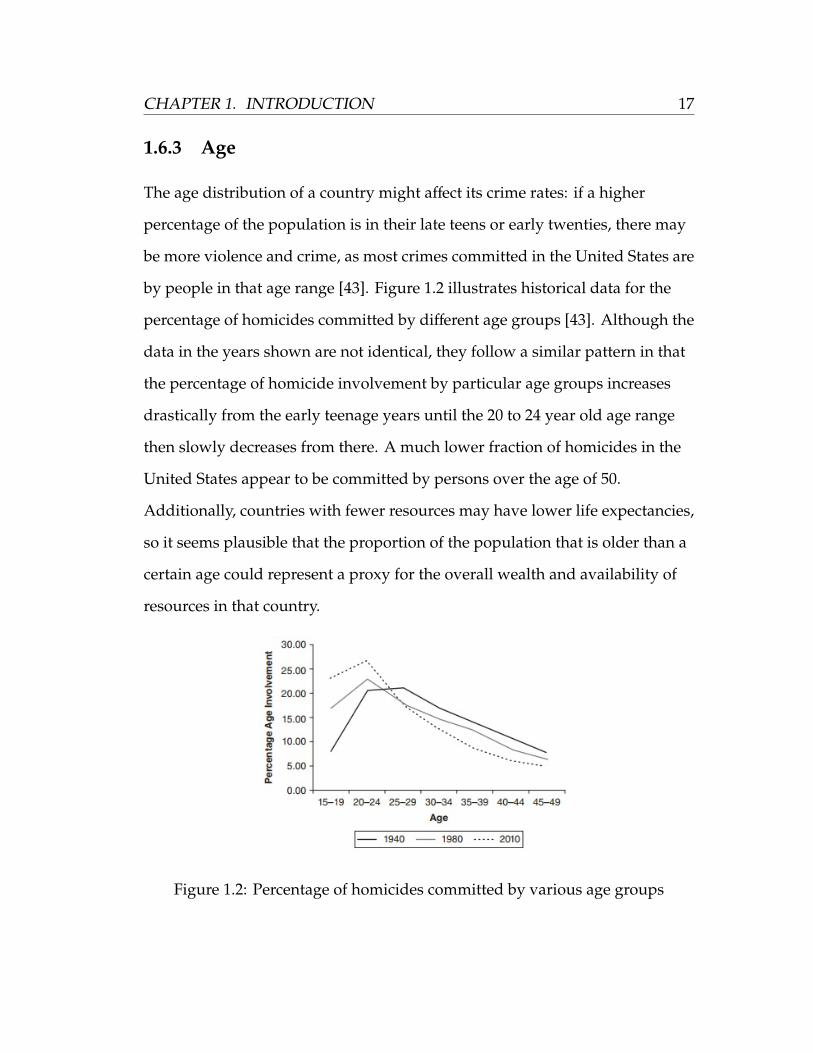
The age distribution of a country might affect its crime rates: if a higher
percentage of the population is in their late teens or early twenties, there may
be more violence and crime, as most crimes committed in the United States are
by people in that age range [43]. Figure 1.2 illustrates historical data for the
percentage of homicides committed by different age groups [43]. Although the
data in the years shown are not identical, they follow a similar pattern in that
the percentage of homicide involvement by particular age groups increases
drastically from the early teenage years until the 20 to 24 year old age range
then slowly decreases from there. A much lower fraction of homicides in the
United States appear to be committed by persons over the age of 50.
Additionally, countries with fewer resources may have lower life expectancies,
so it seems plausible that the proportion of the population that is older than a
certain age could represent a proxy for the overall wealth and availability of
resources in that country.
Figure 1.2: Percentage of homicides committed by various age groups

18 CHAPTER 1. INTRODUCTION
1.6.4 Gender
For all countries with available data on the subject, males have a notably
higher arrest rate for almost every crime than females (save prostitution, for
which females have a much higher arrest rate) [4]. This is particularly true for
serious crimes such as homicide and aggravated assault, for which females
only account for approximately 15% of the total arrests in the United States.
Female property crime arrests are even lower, with less than 10% of the United
States arrests being female [4]. Additionally, it has been shown that females are
less likely to be repeated offenders [4]. Even though these rates have only been
proven true in the United States, it seems possible that countries with a higher
ratio of males to females may have higher overall crime rates. However, since
most countries are likely to have nearly perfect 1:1 gender ratios, there may
not be enough of a difference between the percentage of males and females in
any given country to have a genuine effect on its crime rates.

Chapter 2
Methodology
This chapter discusses the techniques of analysis that were used in
determining the factors that have the most significant influence on worldwide
crime rates and building aggregate crime models from these factors. Methods
detailed in this chapter include data standardization, linear regressions,
stepwise regressions, principal component analysis, residual analysis, random
forests of regression trees, and generalized linear models.
2.1 Data Standardization
Standardizing a dataset re-scales each predictor so that it has a mean of zero
and a standard deviation of one. The standardized form of a random data
sample is often called its z-score. Before standardizing data, we must calculate
the variance of the sample. For a random data sample X with n points
19
20 CHAPTER 2. METHODOLOGY
(x1, x2, · · · , xn) and mean µx, the formula for the variance [42] is:
varX =
∑ni=1(µx − xi)2
n − 1(2.1)
The variance of a sample of data is simply the square of its standard deviation.
If we let µX be the mean of sample X, varx be the variance of X, and xi ∈ X be
the ith individual observation (for i = 1, 2, · · · ,n), then the new standardized
value zi for each element in X [14] will be given by:
zi =xi − µX√
varX(2.2)
The standardization of a data set allows the analysis results for each predictor
to be compared more easily with one another because it puts all the factors on
the same scale [14]. For example, if the values of all the observations in one
predictor range from 0 to 1 and those in another predictor range from −500 to
500, it can be rather difficult to analyze the significance their linear regression
slopes, as their scales are not comparable. Standardizing the data would put
the values of both predictors on the same scale, which would then provide
comparable results. This is desirable down the line because it allows us to
compare model coefficients of every factor: the coefficients with the highest
magnitudes will correspond the most significant factors in the model.

CHAPTER 2. METHODOLOGY 21
2.2 Linear Regressions
Linear regressions estimate the effects of n explanatory data samples
X1,X2, · · · ,Xn on some dependent data sample Y. They find a predicted value
M for each observation of all the dependent variable using the values of the
given predictors. To calculate linear regressions for independent and
dependent variables (in this study, these are the predictive factors and the
crime rates, respectively), a linear equation is built from the values of the
independent variables and then fit to the data. In my regression, I used the
least-squares model to calculate the best-fitting linear equations for the data. A
least-squares model calculates the slope and y-intercept of the linear line that
minimizes the summed squares of the y-axis differences between each data
point and the line [11]. If there are n data points 1, 2, · · · ,n and we let di be the
difference on the y-axis between a linear line and data point i, then the
equation to calculate the line of best fit [11] is:
minn∑
i=1
d2i . (2.3)
The linear equation for the predicted value M of the dependent variable
from n predictors X1,X2, · · · ,Xn and coefficients for the line of best fit
β0, β1, β2, · · · , βn [11] is given by:
M = β0 + β1X1 + β2X2 + · · · + βnXn. (2.4)

22 CHAPTER 2. METHODOLOGY
To use the line of best fit found by a linear regression to calculate the predicted
value Mi for the ith observation of a dataset with m samples and n predictors,
we use the formula shown in Equation 2.5 [11].
Mi = β0 + β1Xi1 + β2Xi2 + · · · + βnXin for i = 1, 2, · · · ,m (2.5)
2.3 Stepwise Regressions
One method that I used to select the factors that seemed to have the greatest
influence on crimes was a stepwise regression, which adds and removes factors
from a predictive model based off of the results of their t-tests. My stepwise
regression included methods to reduce overfitting such as partitioning the
data into testing and training sets and k-fold cross validation.
2.3.1 T-test
A t-test is a ratio of the means of two random samples of data with their
variances taken into account. A t-test is used to compare the means of these
two data samples to determine whether their correlation is significant. If we
have two random data samples X and Y, with µX and µy being their respective
means, nX and nY being their respective number of data points, and varX and
varY being their respective variances (the formula for which can be found in
Equation 2.1), then the equation to find their t-test to determine the strength of
their correlation [42] is:
t =µX − µY√varXnX
+ varYnY
. (2.6)

CHAPTER 2. METHODOLOGY 23
The formula in the denominator of equation 2.6 is also known as the formula
for standard error, which is used to compute a confidence interval for the
difference between the means of both data samples. A confidence interval
calculates the level of certainty of a statistical estimate (a standard confidence
interval is 95%, which means that there is a 95% chance that the sample mean
of a new random sample from the same population would be within that
interval) [2]. In general, a higher t-value indicates a higher correlation between
the data samples [20]. After the t-value of the two sets of data is computed,
they are usually compared to a standard table of significance, which gives its
corresponding p-value. The correlation between two data samples is usually
deemed significant if the p-value is less than 0.05 [42].
2.3.2 Overfitting
A problem that is seen frequently in the realm of model-building is overfitting.
This occurs when a model is built quite accurately for a specific dataset, but
when applied to different data, it loses much of its accuracy (meaning the error
of the model increases). Since models are built directly from data, they often fit
to random noise in that particular dataset, which does not translate to outside
data. There are two methods used in my stepwise regression to combat this:
partitioning the data into two sets (training and testing) and k-fold cross
validation.
To partition the dataset, I randomly split it into training and testing sets at
a 4:1 ratio. In other words, a random 80% of the data is used for training and
the remaining 20% is used for testing. A model is then built from only the data

24 CHAPTER 2. METHODOLOGY
observations in the training set, and this model is then applied to the testing
set to ensure the predictability holds when applied to new data. If the model
error is significantly higher when evaluating the testing set than the training
set, then the model is likely accounting for unwanted noise in the training set.
When modeling data to predict the values of yet-unknown observations of the
dependent variable, a similar technique called validation is often performed. In
this technique, the known data is randomly partitioned into two sets, training
and validation, and the data being used to predict the remaining unknown
dependent values go into the testing set. When this third set is applied, a
model is built from the training data, then validated on the validation set, and
then a the model is applied to predict the the testing data [21]. Since the values
of the dependent variable in the testing set are not known, we cannot calculate
the error of the model, so we use the model error of the validation set as an
approximation for the error of the testing set.
The issue of overfitting can also be resolved by using a k-fold cross
validation (in my analysis, I will be using k = 5 to match the 4:1 training to
testing set allocation ratio). This process randomly splits the data into k smaller
sets (of a roughly equal size), often called folds. Next, k − 1 of these folds are
used as training data from which a model is built, then this model is tested on
the remaining data fold. The folds are then recombined k − 1 more times, so
that each of the folds is used as testing data exactly once, while a model is built
from the data in the other k − 1 folds [21]. Sometimes it can also be helpful to
perform an n-fold (“hold-one out”) cross-validation (where n is the number of
observations in the data), in which n models are built, each of which uses all
the data points but one to predict the value of the remaining data point.

CHAPTER 2. METHODOLOGY 25
2.3.3 Stepwise Regression
A stepwise regression evaluates the effects of each of the predictive factors on
the dependent variable. It adds and removes factors to and from the model
based off the significance of their t-tests. A stepwise regression is a recursive
process, for which predictors are either added or removed at each step, and
the process stops when no more factors can be added because the remaining
are deemed insignificant.
Before starting the regression, p-value thresholds are set for the addition
and removal of factors. In my analysis, I require that a factor must have a
p-value of 0.1 or less to be added and a p-value of 0.15 or more to be removed.
The universal indicator of significance for p-values is 0.05, so I chose 0.1 as the
inclusion value because it provides a margin of freedom–if a factor has a
p-value only slightly higher than 0.05, it will not necessarily be completely
ignored. Similarly, I chose 0.15 as the removal value because it is significantly
higher than 0.05 and, therefore, factors with this high of a p-value are likely to
be insignificant.
To begin the process, zero predictors are included in the stepwise model.
A t-test is then performed on each of the predictors with the dependent
variable and if the factor with the highest t-score has a p-value lower than 0.1,
it is added to the stepwise model; otherwise, the process halts and the model
will include no factors. After the first factor is included, the process is
repeated: this time, the dependent variable is regressed with the variable
selected for the model and each of the other predictors, the t-tests are
performed, and the variable that has the highest t-value is included in the

26 CHAPTER 2. METHODOLOGY
model so long as its p-value is below 0.1. If its p-value is not below 0.1, the
process halts and only the one factor will be included in the model.
Additionally, if the p-value of the first factor increased to a value greater than
0.15 after the second factor was added, then it is removed from the model and
we are left with only the second factor [20]. This process is repeated,
regressing all the current factors in the model against the remaining factors,
adding the factors with the highest t-test values if they have significant
p-values, and removing any current model factors that become insignificant in
the process. The process only halts when there are no remaining factors with
large enough p-values to add [20]. The model at the end of the stepwise
regression contains all the factors that, together, will minimize the model error.
However, it should be noted that there is no guarantee that the model found is
the optimal model, as there could be multiple different combinations of factors
selected from running several stepwise regressions [20].
2.4 Eigenvalues and Eigenvectors
Finding the eigenvalues and eigenvectors of a matrix can tell us important
information about that matrix, which will be further detailed in Section 2.5. If
we have a n × n matrix X, its eigenvalues and corresponding eigenvectors are
some λ and v (respectively) such that Xv = λv. There are many different ways
to find these values, but we will be using a simple linear algebra technique
that uses the determinants of X to find its eigenvalues and then using those
eigenvalues to find their corresponding eigenvectors.

CHAPTER 2. METHODOLOGY 27
To calculate the determinant of X, we use the equation
det(X) =
n∑j=1
xi jXi j (2.7)
where i is a fixed integer between 1 and n, xi j is the entry in row i and column j
of X, and Xi j is (−1)i+ j multiplied by the determinant of the matrix that is the
result of removing the ith row and jth column of the former Xi j [33]. This
equation is often referred to as “expansion by minors.” To find the eigenvalues
λ1, λ2, · · · , λn of X, we use Equation 2.7 to solve det(X − λIn) = 0 where In is the
n × n identity matrix [3]. There are n solutions to this equation because
det(X − λIn) is a polynomial of degree n [3]. However, some solutions might be
complex or repeated: complex and duplicate values are disregarded.
When we have the n eigenvalues of X (not all of which are necessarily
distinct), for each λi (where i = 1, 2, · · · ,n), we solve
(X − λiIn)vi = 0 (2.8)
for vi, which represents its corresponding eigenvector [3].
2.5 Principal Component Analysis
When there is a high correlation between predictors in a model, there are often
underlying similarities among them, and including many similar factors in the
model can result in overfitting. Additionally, the sheer size of some raw
datasets can be nearly impossible to work with, as there are often far too many

28 CHAPTER 2. METHODOLOGY
factors to directly analyze and model. One way to fix this problem is by the
use of Principal Component Analysis (PCA) to identify patterns and underlying
correlations between factors. These patterns are then used to combine the
original factors in a way that results in fewer predictors, making the data
easier to work with [37].
PCA is a multi-step process that involves several linear algebra techniques.
The process is as follows: a matrix of predictors to be combined are
standardized (let us call this matrix W) and a covariance matrix is formed from
these predictors. Then the eigenvalues and eigenvectors of the covariance
matrix are found, the eigenvalues are sorted from largest to smallest in
magnitude, and the k eigenvectors with the highest corresponding eigenvalues
(where k is the desired number of final predictors) are put into a new matrix Z.
Finally, calculating W × Z produces the k new columns of predictors [37].
2.5.1 Covariance Matrices
A covariance matrix C is an n × n matrix that calculates the covariance
between X and Y and places that value in its ith row and jth column. Let W be
an m × n data matrix such that m is the number of data points and n is the
number of predictors. To perform a PCA on W, we must first standardize the
data using the formula given in Equation 2.2. Next, to find the covariance
matrix, we must first calculate the covariance between each data sample. The
covariance between two samples indicates the strength of their correlation: a
higher covariance implies a stronger correlation and a covariance of zero
indicates that the samples are statistically independent from one another [44].

CHAPTER 2. METHODOLOGY 29
Let X be the ith predictor and Y be the jth predictor in W, both with m data
points and respective sample means µX and µY. The equation for the
covariance of X and Y [10] is given by
Cov(X,Y) =
∑mi=1(X − µX)(Y − µY)
m − 1(2.9)
The covariance between each predictor is calculated and placed into the
covariance matrix C (the covariance between predictor i and predictor j is
placed in the ith row and jth column of C).
2.5.2 New Predictors
Next, we find the eigenvalues and eigenvectors of C (the process for which is
detailed in Section 2.4) and we sort the real eigenvalues from largest to
smallest in magnitude. If we want k new predictors from the PCA, we select
the eigenvectors that correspond to the k eigenvalues with the greatest
magnitudes, combine them into a new matrix Z (the eigenvector with the
eigenvalue of greatest magnitude is in column 1, that with the second highest
is in column two, and so on), and multiply the original data matrix W by this
new matrix Z [37] so that we get:
A = W × Z (2.10)
Each column of this m × k matrix A represents a new predictor that is a
combination of the original predictors.

30 CHAPTER 2. METHODOLOGY
2.6 Normal Distributions
A normal distribution takes of the form of a bell curve in which data is
distributed symmetrically around the sample mean, with the majority of the
data observations close to the mean and fewer and fewer observations as the
distance from the mean increases. The probability density function of a
normal distribution is
f (y) =1√
2πσe−
12 ( y−µ
σ )2(2.11)
where µ is the mean of the data and σ is the standard deviation. This formula
calculates the probability that the value of any given observation in a normally
distributed random data sample will equal y.
Normal distributions occur naturally in many situations: many random
samples of data are at least somewhat normal. Normal distributions indicate
the portion of the data that is distributed within a certain standard deviation
of the mean: 68% falls within one standard deviation, 95% falls within two,
Figure 2.1: Illustration of a normal distribution

CHAPTER 2. METHODOLOGY 31
and 99.7% falls within three [12]. A visual representation of these normal
distribution distributions on a bell curve can be found in Figure 2.1 [19].
2.7 Residual Analysis
The equation to find the residuals R of a dependent data sample Y is given in
Equation 2.12, where Ri is the residual at data point i, yi ∈ Y is the actual value
of the dependent variable at i, and Mi is the value predicted forY at that
observation found by the linear regression of some predictor with Y.
Ri = yi −Mi (2.12)
Performing a residual analysis of one or more predictors and a dependent
variable can reveal whether a linear model is the best fit for a specific dataset.
A residual analysis evaluates patterns in the residual plot of a data sample and
compares them to those of samples that are well-fit for linear models. The
residual plot of a predictor displays the values of the independent variable on
the x-axis and the residual values of the dependent variable Y on the y-axis.
Since the residual values can be either positive or negative, they are plotted
around the horizontal axis to observe the distribution of positive and negative
values. If the residual values are randomly dispersed around the horizontal
axis (signifying that there is no clear pattern among them), then a linear
regression model may be an appropriate fit for the data [7]. An example of this
can be found in Figure 2.2 [7]. A random residual distribution as seen in this
figure implies that the data values likely have a relatively normal distribution
32 CHAPTER 2. METHODOLOGY
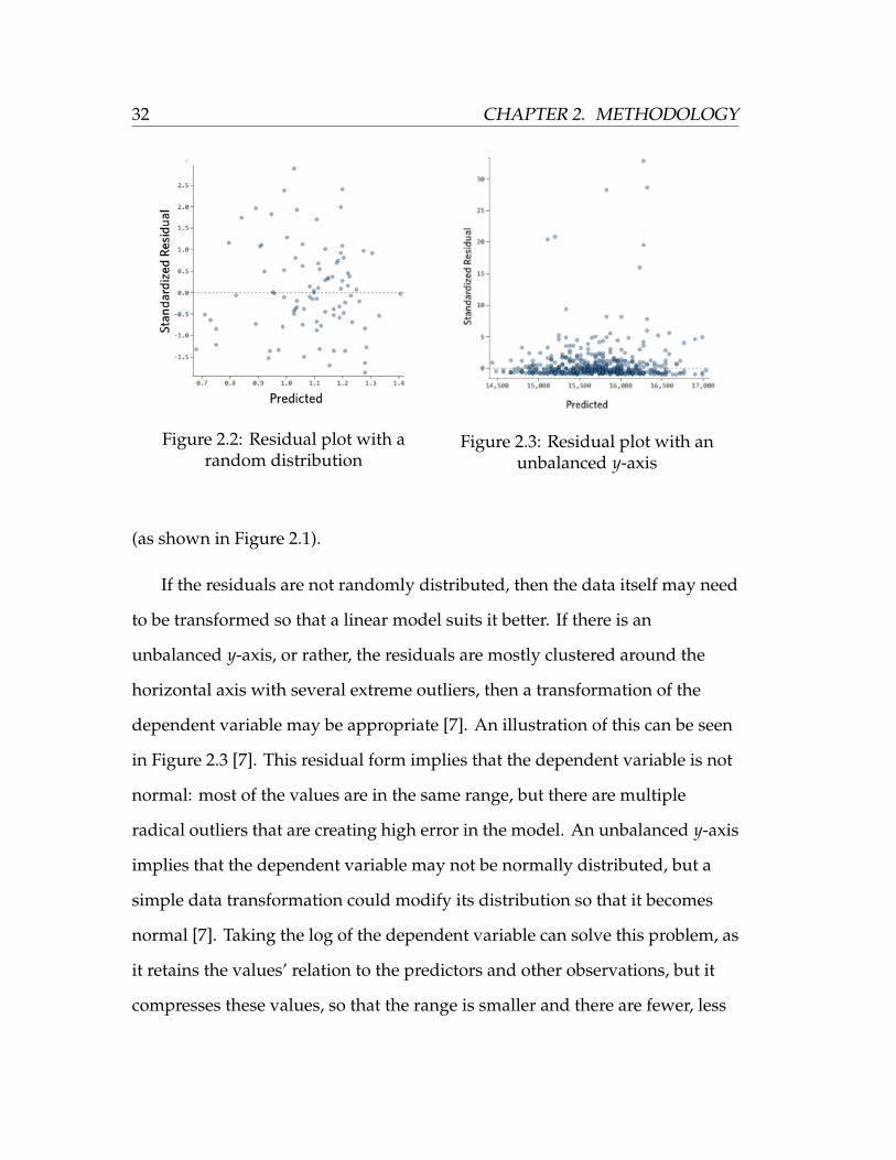
Figure 2.2: Residual plot with arandom distribution
Figure 2.3: Residual plot with anunbalanced y-axis
(as shown in Figure 2.1).
If the residuals are not randomly distributed, then the data itself may need
to be transformed so that a linear model suits it better. If there is an
unbalanced y-axis, or rather, the residuals are mostly clustered around the
horizontal axis with several extreme outliers, then a transformation of the
dependent variable may be appropriate [7]. An illustration of this can be seen
in Figure 2.3 [7]. This residual form implies that the dependent variable is not
normal: most of the values are in the same range, but there are multiple
radical outliers that are creating high error in the model. An unbalanced y-axis
implies that the dependent variable may not be normally distributed, but a
simple data transformation could modify its distribution so that it becomes
normal [7]. Taking the log of the dependent variable can solve this problem, as
it retains the values’ relation to the predictors and other observations, but it
compresses these values, so that the range is smaller and there are fewer, less

CHAPTER 2. METHODOLOGY 33
Figure 2.4: Residual plot with an unbalanced x-axis
extreme outliers [7]. If the logarithmic form of a predictor is normal, it is often
referred to as “log-normal”. After taking the log of the dependent variable, a
linear model may fit the data more appropriately than before.
It is also common for a residual plot to have an unbalanced x-axis. In this
case, the residuals are mostly clustered along the vertical axis with a few
significant outliers. An illustration of this can be seen in Figure 2.4 [7]. In some
cases, a residual plot in this form can be disregarded: it sometimes implies that
there is nothing wrong with the model. However, other times it means that the
model can be improved by transforming the independent variable, often by
taking its log or squaring it [7]. In this case, as before, a simple data
transformation of a predictor could modify it so that it has a more normal
distribution, which could help it fit better in a linear model. To determine
which step to take if an unbalanced x-axis is encountered in a residual plot is
to experiment by transforming the independent variable in different ways and
observing whether or not the model error decreases.

34 CHAPTER 2. METHODOLOGY
However, if the residual plot of the model is not similar to the residual
plots shown in Figures 2.2, 2.3, or 2.4, or if a histogram of the data
distributions do not match the normal distribution shown in Figure 2.1, then a
linear model may not be a good fit for that particular dataset. This could
suggest that another factor should be added to the model or that a nonlinear
model may be a better overall fit for the dataset.
2.8 Machine Learning
Machine learning algorithms are a class of data modeling techniques in which
computers recognize and evaluate data and build models from that data using
artificial intelligence. Computers use iterative methods to adapt to new data
and make their own decisions regarding its categorization [13]. The specific
machine learning techniques that will be used in this study are binary
regression trees and random forests, which are an extension of regression trees.
2.8.1 Decision Trees
Both of the machine learning techniques in this study are forms of decision
trees, which play a key role in data classification. Decision trees partition data
into two or more categories based on previously established splitting criteria
[18]. The algorithm begins with a full dataset, then the splitting criteria
partitions the data into different categories, and from there, the data is often
partitioned into even more categories. This process continues until the data
has been fully partitioned (or when the splitting criteria is no longer

CHAPTER 2. METHODOLOGY 35
Figure 2.5: Binary decision tree with terminology
applicable). Each point at which a split value is created and more data is
partitioned is called a node. A binary decision tree is a decision tree that has at
most two partitions from any given node. Figure 2.5 illustrates a binary
decision tree labelled with the proper node terminology. The root node is the
node at the very beginning of the algorithm. This node evaluates the entire
dataset before it is partitioned. Each decision tree contains exactly one root
node. Following the root node are the decision nodes. Each decision node
evaluates a set of data that has been previously partitioned at least once,
creates a new split value, and proceeds to divide the data further. Finally, a
terminal node is the last step in a decision tree algorithm: the data from this
path of the decision tree has been fully partitioned. Hence, the data in each of
the terminal nodes represent the final classification of the data [18].

36 CHAPTER 2. METHODOLOGY
2.8.2 Regression Trees
A binary regression tree partitions the data at optimal split values based on a
process called binary recursive partitioning. This algorithm is similar to a
decision tree in that the root node evaluates the entire dataset, the data is split
into decision nodes based off of an original split value, and the terminal nodes
contain the final subsets of the data and generate the predicted model values
for these subsets. Equation 2.13 shows the formula to calculate the optimal
split value (the value that will generate the least amount of model error) for
each partition in factor i, where n is the number of data points in the current
partition X, µX is the sample mean of the partition, and xi ∈ X is the actual
value for a particular data point.
split value = minn∑
i=1
(µX − xi)2 (2.13)
This formula is applied to each of the individual factors under consideration
and the factor with the smallest split value is used for the partition [13]. This
process continues until each path contains a user-specified number of decision
nodes. If the factor is categorical (meaning there are a finite number of
categories into which each observation is already classified), the data is
partitioned based on the category to which they belong. If the factor is
continuous, all the data observations that have values less than that particular
split value are partitioned in one group, and the rest are partitioned into the
other group [13]. When a data observation goes through a complete binary
regression tree, it starts at the root node, and, for each partition, follows the
path that matches the observation’s value against the partition’s split value at

CHAPTER 2. METHODOLOGY 37
that factor. The value at the terminal node that an observation ends up at is the
predicted model value for that particular observation.
A major issue with many binary regression trees is overfitting. When data
is entered into a regression tree to be partitioned, the split values of the tree
will be biased toward that data. In other words, the tree fits very closely to the
information in the given data (including all the random noise), but this overly
close fit may not hold its predictive value as well for any new data. For this
reason, it is very important to use training and testing data when modeling
with this method to observe how much of the model’s accuracy can be
attributed solely to overfitting.
To combat this overfitting problem, there is a built-in process for most
binary regression trees called pruning. Pruning evaluates each terminal node
and decides whether any should be eliminated. There are multiple methods to
prune, but the method that will be used in this analysis is cross-validation,
which is detailed in Section 2.3.2. This method tests all the different
combinations of adding and removing terminal nodes until the
cross-validation error is at a minimum [30]. If a terminal node is removed, the
previous decision node becomes, itself, a terminal node, and is then considered
among the combinations of terminal nodes for the cross-validation testing.
2.8.3 Random Forests
The random forest machine learning algorithm is the next step in the field of
regression trees. In this method, individual regression trees are built for
multiple random subsets of the data. When new data is input, it is evaluated

38 CHAPTER 2. METHODOLOGY
by each of the regression trees and its final predictive value is the average of
the predictions from all the trees [25]. For efficiency and to avoid bias, the
individual trees are not pruned as they would be in single regression tree
modeling. Additionally, to reduce overfitting and to avoid trees that are too
similar, not every factor is considered for each tree when the algorithm
searches for the optimal split value. If n is the total number of factors in the
dataset, I set the number of factors randomly selected to be considered for
each tree as n3 , as it is the default in MATLAB [25]. This step ensures more
diversity among the regression trees.
2.9 Generalized Linear Models
Another method that will be used to model aggregated crime rates in this
study will be generalized linear models. Generalized linear models predict the
ith value of the dependent variable yi based off of some function η of its
independent variables xi1, xi2, · · · , xin. This study will use the linear regression
model form of generalized linear models (refer to Section 2.2 for further details
about linear regression models).
A generalized linear model has three main components: systematic,
random, and link [1]. The systematic component determines the specific linear
combination in which the model factors are applied to predict the dependent
variable µY. The random component adds random error to the model by
applying a probability distribution to the dependent variable. The probability
distribution is specific to the model type. The linear regression model assumes
that every data sample has a normal distribution. Finally, the link component

CHAPTER 2. METHODOLOGY 39
ties the systematic and error components together by applying a function η to
the predictors to best capture how the dependent variable responds to its
independent variables. A linear regression model uses the identity function as
the link (η = µY) [1].
Generalized linear models do make assumptions about the data that could
generate error in the results. First, it assumes that all the factors are completely
uncorrelated from one another, which is not likely the case [1]. Many factors
are likely to have some degree of correlation with at least a few other factors.
Second, it assumes a probability distribution for the dependent variable [1]. It
is likely that there is some form of distribution for the dependent variable, but
this is not guaranteed. When a model is created from a linear model, the
predicted values for the dependent variable follow a normal distribution.

40 CHAPTER 2. METHODOLOGY

Chapter 3
Results
This section specifies the distinct predictors that were analyzed from the
categories discussed in Chapter 2 and the results of the modeling of these
predictors on aggregated worldwide crime rates. Unless otherwise specified,
every factor was standardized for this analysis (see Section 2.1 for details
about the standardization process), thus these results are displayed in
comparable units.
3.1 Data Sources
The data used in this study came from a variety of sources. 196 countries from
around the world were included in the dataset, but not all countries had data
available for every factor. Additionally, there were two regions of China
included, Macau and Hong Kong, but for the sake of simplicity I will refer to
them as countries throughout this study.
I considered two categories of crime rate (the dependent variable) in this
41

42 CHAPTER 3. RESULTS
Figure 3.1: Distribution of the rawhomicide rates
Figure 3.2: Distribution of the loggedhomicide rates
study: homicide rates and burglary and housebreaking rates. These rates were
in the form of annual number of cases per 100,000 population. This data came
from knoema [17], a worldwide data atlas that presents statistics from every
country in the world. The crime rates given are the most recent years available
for each country. 197 of the 198 countries had homicide rates available, but
only 103 countries had burglary and housebreaking rates available. The
homicide rates ranged from 0.2 to 74.6 cases per year and the burglary and
housebreaking rates ranged from 1.3 to 947.2 cases.
Unless otherwise specified, the logarithms of both crime rates were used
for all analyses performed in this section so that they had a more normal
distribution. This allowed for a better fit in a linear model. Figure 3.1 shows a
histogram of the distribution of the raw homicide rates and Figure 3.2 shows
the distribution of the logged rates. Each observation represents a country and
the red line in Figure 3.2 represents a normal distribution of the data. The
logged homicide rates appear to be much more normal than the raw rates,
suggesting that the homicide rates are log-normal. It should be noted,

CHAPTER 3. RESULTS 43
Figure 3.3: Distribution of the rawburglarly/housebreaking rates
Figure 3.4: Distribution of the loggedburglary/housebreaking rates
however, that the logged rates do not perfectly match the true normal
distribution illustrated in Figure 2.1.
Similarly, Figure 3.3 shows a histogram of the distribution of the raw
burglary and housebreaking rates and Figure 3.4 shows the distribution of the
logged rates. It appears that the burglary and housebreaking rates are also
log-normal. As we saw with the homicide rates, even though the logged
burglary and housebreaking rates are much more normal than the raw rates,
but they are not perfect.
The data for many of the attributes in this study also came from knoema
[17]. The full list of factors considered that came directly from knoema can be
found below. All ratios were represented in the form of percentages.
1. Poverty: the unemployment ratio, the poverty ratio below $1.90 per day,
the poverty ratio below $3.10 per day, the poverty ratio below the
national poverty line, the rural poverty ratio, the urban poverty ratio
2. Income inequality: the Gini index

44 CHAPTER 3. RESULTS
3. Education: annual expenditure on education as a share of GNI, annual
total public expenditure on education, the adult literacy ratio, the gross
enrollment ratio in primary education, the completion ratio for primary
education, the gross enrollment ratio in secondary education, the gross
graduation ratio for secondary education, the female student ratio in
primary education, the female student ratio in secondary education
4. Other factors: GDP per capita, GDP growth, GDP per capita growth, the
population ratio for ages 0-14, the population ratio for ages 65 and older,
the female population ratio
The values of $1.90 and $3.10 per day for the poverty rates were those that
were attached to the data on knoema. It is not specified why these particular
values were chosen.
As discussed in Section 1.3, the government quality data came from the
Worldwide Governance Indicators [31] and was divided into six indices: Voice
and Accountability, Political Stability and Absence of Violence or Terrorism,
Government Effectiveness, Regulatory Quality, Rule of Law, and Control of
Corruption.
The ethnolinguistic fractionalization data came from two sources. I
considered the ELF index mentioned in Section 1.4 [38] as well as the three
separate indices for ethnic, linguistic, and religious fractionalization [22].
I created a binomial variable for whether a country is located in Latin
America or the Caribbean from consulting a list of countries located in that
area [8]. For this category, I gave every country a 1 if it was on the list and a 0
otherwise.

CHAPTER 3. RESULTS 45
I got drug consumption data from the World Health Organization [16] and
the World Drug Report [15]. The data in this category included the number of
pure liters of alcohol consumed annually per capita (for ages 15 and older) and
the percentage of a country’s population that admitted to consuming cannabis
(for ages 15-64). However, these values may not accurately represent the
actual rates of consumption, as it is possible that many cannabis users would
not admit to its use, as it is illegal in many countries.
3.1.1 Assumptions
There were some assumptions that I made about the data to facilitate my
analysis.
First, I assumed that any and all data that came from surveys was reliable,
which may not actually be the case. This includes the government quality and
drug consumption data. The possible reliability of both these factors was
previously discussed in Sections 1.3 and 3.1, respectively.
Second, the data for each country provided by knoema were given by the
most recent year in which data is available, so I assumed that these values are
representative of each country’s usual crime rates. This may not necessarily be
the case, as there may have been special circumstances that year that caused
an increased or decreased amount of crime from the usual amount.
Additionally, the year in which data is represented for a single factor may vary
from country to country.

46 CHAPTER 3. RESULTS
3.2 Linear Regressions
To perform a single variable linear regression in MATLAB, I used the regress
command and input the crime rate that I was examining with the predictor
that I was considering. This output two values: an estimate of the y-intercept
of the regression line (β0) and an estimate of the slope (β1), both of which were
calculated using the least-squares model discussed in Section 2.2. For a linear
regression with some predictor X, for each observation i, the regression
estimate Mi for every value xi ∈ X was given by Mi = β0 + β1xi.
Performing linear regressions on the crime rates yielded surprising initial
results: almost every factor had opposite regression slope directions for the
two different crimes. The only factors that had matching slope directions were
expenditure on education as a share of GNI (both positive), the religion index
(both positive), and the female population ratio (both positive).
A linear regression of homicide rates with burglary and housebreaking
rates yielded a slope of −0.12. This indicates that there was actually a fairly
low correlation between the two types of crime in this study. Additionally, the
relationship they did have appears to be negative: as a country’s homicide rate
increases, its burglary and housebreaking rate may be prone to slightly
decrease. This does not follow intuition, as one might expect both crime rates
to have a strong, positive relationship. However, these unusual results could
partially explain why most of the factors had opposite coefficient signs in their
respective linear regressions.
Because the predictors were standardized, the strength of their linear
regression slopes with the individual crime rates are shown in comparable

CHAPTER 3. RESULTS 47
units. This means that the regressions that generated stronger slopes with a
particular crime rate had a higher correlation with that crime.
3.2.1 Homicide Slopes
The factor that appeared to have the strongest correlation with homicide was
the Gini index with a linear regression slope of 0.61. The positive slope
indicates that countries with more income inequality (represented by higher
Gini indices) are likely to have higher homicide rates as well. Figure 3.5 shows
the regression slope of the raw Gini indices and logged homicide rates. The
blue dots represent individual countries and the red line represents the
least-squares linear regression line. These results match our expectations: we
predicted in Section 1.1 that income inequality would have a higher
correlation with crime than poverty alone. Table 3.1 shows the next five factors
that had the strongest slopes when regressed with homicide rates. It should be
noted that four of these factors are governance indicators. All the governance
Figure 3.5: Linear regression of the Gini index and homicide rates

48 CHAPTER 3. RESULTS
Factor Linear Regression Slope
Government Effectiveness −0.54Rule of Law −0.53
Regulatory Quality −0.49Control of Corruption −0.47
Population ratio for ages 65 and older −0.47
Table 3.1: Select factors and their linear regression slopes with homicide rates
indicators had negative coefficients, which follows our prediction in Section
1.3: countries with higher government indices tend to have lower aggregate
homicide rates. A full list of linear regression slopes for each factor with
homicide can be found in the Appendix.
3.2.2 Burglary and Housebreaking Slopes
The linear regression slopes of the factors with burglary and housebreaking
rates tended to be slightly stronger than those for the factors with homicide
rates. Because there were significantly fewer countries that had available
burglary and housebreaking rates than there were that had available homicide
rates, the regression results may not be quite as accurate.
The factor that had the strongest regression slope with burglary and
housebreaking was the gross enrollment ratio in secondary education with a
coefficient of 0.79. The positive slope indicates that an increased enrollment in
secondary education is actually correlated with higher burglary and
housebreaking rates, which does not necessarily follow intuition. Figure 3.6
shows the linear regression line for the unstandardized enrollment in
secondary education with the logged burglary and housebreaking rates. The

CHAPTER 3. RESULTS 49
Figure 3.6: Linear regression of the secondary education enrollment ratio andburglary and housebreaking rates
blue dots represent individual countries and the red line represents the
least-squares linear regression line. Notice that some of these ratios exceed
100: this is because over-aged and under-aged students entering school early
or late are included, as are students that have repeated a grade [17]. Table 3.2
shows the next five factors that had the strongest linear regression slopes with
burglary and housebreaking rates. A full list of factors and their linear
regression slopes with burglary and housebreaking rates can be found in the
Appendix.
Factor Linear Regression Slope
Voice and Accountability 0.74Poverty Ratio below $1.90 per day −0.74
Female student ratio in primary education 0.73Gross graduation ratio in secondary education 0.66
Adult literacy ratio 0.64
Table 3.2: Select factors and their linear regression slopes with burglary andhousebreaking rates

50 CHAPTER 3. RESULTS
We can see that these results are quite different from the homicide
regression results (in addition to having opposite coefficient signs for most
factors). Poverty appears to have a stronger correlation with burglary and
housebreaking than income inequality (which only had a coefficient of −0.38),
which was the opposite of what we found in the homicide regressions.
Additionally, the government quality indicator that had the highest
correlation with burglary and housebreaking was Voice and Accountability,
which was the indicator that had the lowest correlation with homicide.
3.3 Residual Analysis
Next, I evaluated each factor to determine whether a data transformation
would be appropriate. To do so, I performed two steps for each factor:
1. I performed a linear regression with both crime rates. I then made a
residual plot of this model to see if the residual distribution was random
(as detailed in Section 2.7).
2. I created a histogram of the distribution of the data to observe whether it
somewhat matched a normal distribution.
I then transformed the factors that did not have random residual plots or
semi-normal distributions. To see what kind of transformation would
generate the most significant results, I tested these factors with three types of
transformations: logarithmic, square root, and square. I then evaluated
whether the transformed variables had a stronger correlation with the crime
rates by standardizing them and observing whether their linear regression

CHAPTER 3. RESULTS 51
slopes were stronger than before they were transformed, and, if so, which
transformation generated the strongest slope. All factors transformed in this
section were analyzed and modeled in their transformed state for the
remainder of the study.
3.3.1 Residual Plots with Homicide Rates
The factors that did not have a random residual plot for their linear regression
models with homicide rates were: the poverty ratio below $1.90 and $3.10 per
day, expenditure on education as a share of GNI, the adult literacy ratio, the
completion ratio for primary education, the gross enrollment ratio in primary
education, the female student ratio in secondary education, GDP per capita,
GDP per capita growth, and the female population ratio. After applying the
three types of transformations mentioned above to each of these factors, I
found that the only transformation that generated a significant improvement
for any of the factors was a logarithmic transformation. With this
transformation, the slopes of two factors were improved: the poverty ratio
below $1.90 per day slope increased from 0.12 to 0.28 and the poverty ratio
below $3.10 per day slope improved from 0.13 to 0.28. The logarithmic
transformation of these factors produced a better overall fit with the homicide
data and gave them a more normal distribution. The remaining factors were
not significantly improved by any of the transformations.
To further evaluate the transformed factors, I created residual plots with
the logged factors against the logged homicide rates to see whether they
became random, as desired. Figure 3.7 shows the residual plot of the unlogged

52 CHAPTER 3. RESULTS
Figure 3.7: Residual plot of unloggedpoverty ratios (below $1.90 per day)
Figure 3.8: Residual plot of loggedpoverty ratios (below $1.90 per day)
poverty ratio below $1.90 per day regressed with homicide. Each blue dot
represents a residual value (the value predicted by the regression subtracted
from the actual value). We can see that it resembles the example residual plot
with the unbalanced x-axis illustrated in Figure 2.4. Figure 3.8 shows the
residual plot of the logged poverty rates regressed with logged homicide rates.
This figure has a mostly random distribution of residuals, as illustrated in
Figure 2.2, which was desired. Similar residual results were found for the
poverty ratio below $3.10 per day.
As we saw in Section 3.1 with the log-transformed crime rates, taking the
log of these factors produced a more normal distribution (implying that these
factors are log-normal), which could potentially allow them to be more
effective in a linear model. Figure 3.9 shows the distribution of raw poverty
rates and Figure 3.10 shows the distribution of logged poverty rates. Each
observation represents a country and the red line in Figure 3.10 represents a
normal distribution of the data. Though the log-transformed poverty ratio
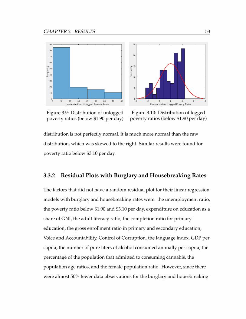
CHAPTER 3. RESULTS 53
Figure 3.9: Distribution of unloggedpoverty ratios (below $1.90 per day)
Figure 3.10: Distribution of loggedpoverty ratios (below $1.90 per day)
distribution is not perfectly normal, it is much more normal than the raw
distribution, which was skewed to the right. Similar results were found for
poverty ratio below $3.10 per day.
3.3.2 Residual Plots with Burglary and Housebreaking Rates
The factors that did not have a random residual plot for their linear regression
models with burglary and housebreaking rates were: the unemployment ratio,
the poverty ratio below $1.90 and $3.10 per day, expenditure on education as a
share of GNI, the adult literacy ratio, the completion ratio for primary
education, the gross enrollment ratio in primary and secondary education,
Voice and Accountability, Control of Corruption, the language index, GDP per
capita, the number of pure liters of alcohol consumed annually per capita, the
percentage of the population that admitted to consuming cannabis, the
population age ratios, and the female population ratio. However, since there
were almost 50% fewer data observations for the burglary and housebreaking

54 CHAPTER 3. RESULTS
Factor Unlogged Slope Logged Slope
Unemployment ratio 0.15 0.23Expenditure on education as share of GNI 0.52 0.63Completion ratio for primary education 0.32 0.40
Female student ratio in primary education 0.73 0.79GDP per capita 0.37 0.67
Table 3.3: Select factors and their linear regression slope improvements withburglary and housebreaking rates
rates than for the homicide rates, the distributions and residual plots were
much more erratic.
I applied the same three types of transformations introduced in Section
3.3.1 (logarithmic, square root, and square) to these factors to determine
whether a stronger linear regression slope could be generated. As with
homicide, I found that only certain factor transformations yielded significant
results, and all of these significant transformations were logarithmic. Table 3.3
shows the improvements that were made to the slopes of the linear regressions
of certain logged factors and burglary and housebreaking rates.
3.4 Principal Component Analysis
To perform Principal Component Analyses (PCA) in MATLAB, I used the pca
command. This command takes one input: a matrix containing only the
factors to be combined. I designed my code so that each separate PCA would
output the principal component variances and one new data column of
combined predictors.
I could not perform a PCA on the entire dataset of predictors, as there were
too many observations missing. Thus, I selected factors that seemed to have

CHAPTER 3. RESULTS 55
high correlations and used the PCA to combine those.
To select factors to combine in a PCA, I observed the relationships between
factors and determined which factors had high correlations with each other. I
approximated the strength of the relationship between factors by performing a
linear regression on two factors and examining the strength of the slope. It
should be noted here that since this was an entirely manual process, I did not
test every possible combination of factors and it is therefore likely that there
were strong factor relationships that I did not include among the
combinations. The nine factor combinations on which I performed a PCA to
merge into one column are:
1. The urban poverty ratio and rural poverty ratio
2. The female enrollment ratio in primary education and gross enrollment
ratio in primary education
3. The gross enrollment ratio in secondary education and gross graduation
ratio in secondary education
4. The female student ratio in primary education and female student ratio
in secondary education
5. Voice and Accountability and Government Effectiveness
6. Voice and Accountability, Government Effectiveness, and Political
Stability
7. The population ratio for ages 0-14 and population ratio for ages 65 and
older

56 CHAPTER 3. RESULTS
8. GDP per capita and GDP per capita growth
9. The number of pure liters of alcohol consumed annually per capita and
the percentage of the population that admitted to consuming cannabis
Next, I tested the new data produced by the PCA to see whether it would
be more beneficial to the model to leave the original factors or to replace them
with the new data. To do so, I performed a linear regression on each of the
new data columns with both homicide rates and burglary and housebreaking
rates. I would then decide to replace the original data with the new data if the
slope was stronger for both of the crime rates in the new data. If the new data
was only stronger for one of the crime rates, I would add it to the dataset and
leave the original data as well, making a note not to use the new data and
original data in the same predictive model.
Most of the factor combinations yielded insignificant results when I
attempted a PCA on them. In almost every case, one of two things happened.
Sometimes the new data would be almost identical to one of the factors (except
perhaps on a slightly different scale), so using the new data would be pointless.
Other times, the new data would be a proper combination of both factors, but
its correlation with both crime rates would be weaker than those of its original
components, so using it might reduce the accuracy of the final model.
The only factor combination that produced successful results was the final
combination listed: the number of pure liters of alcohol consumed annually
per capita and the percentage of the population that admitted to consuming
cannabis. This combination produced a stronger linear regression slope with
both crime rates than either of its individual components did. Table 3.4 shows

CHAPTER 3. RESULTS 57
Crime Component #1 Component #2 Combined Data
Homicide −0.18 −0.14 −0.25Burglary and Housebreaking 0.56 0.31 0.57
Table 3.4: Linear regression slopes of new data generated by a PCA comparedwith those of its component factors
the linear regression slopes for both crimes with the new data after the PCA to
those with the original components. Let Component #1 represent the number
of pure liters of alcohol consumed annually per capita and Component #2
represent the percentage of the population that admitted to consuming
cannabis. I did leave the original two factors in my dataset as a precaution,
even though this did, admittedly, somewhat negate the purpose of performing
the PCA.
3.5 Trends in Individual Regions
Next, I evaluated the data to see if the impact of certain predictors on crime
varied in different parts of the world.
First, I found the sample mean and standard deviation of each predictor at
a worldwide level. For each region, I found the mean of every raw factor to
see if any of them were at least one standard deviation away from the global
mean. This told me whether that region differed significantly from the rest of
the world for any of the predictors.
Additionally, for each region I performed a linear regression on every
standardized factor with both of the crime rates. This showed me which
factors appeared to have a heavier impact on certain regions.

58 CHAPTER 3. RESULTS
3.5.1 Worldwide Averages
The global average homicide rate was 7.66 annual cases per 100,000
population with a standard deviation of 11.42. The “country” with the lowest
recorded homicide rate was Macau, a southern region of China, with a rate of
0.2, and the country with the highest rate was Honduras, a country in Latin
America, with a rate of 74.6.
The global average burglary and housebreaking rate was 171.76 cases per
100,000 population with a standard deviation of 284.03. The country with the
lowest recorded burglary and housebreaking rate was Cameroon, a country in
Africa, with a rate of 1.3, and the country with the highest rate was Saint Kitts
and Nevis, a country in the Caribbean, with a rate of 947.2.
A full list of the worldwide means and standard deviations for each factor
can be found in the Appendix.
3.5.2 Regional Trends
To see how various predictors affected regions differently, I split the data into
four groups: Latin America and the Caribbean, Europe, Africa, and Asia.
Countries that are not located in these regions were not included in this
section of the study.
Latin America and the Caribbean
I predicted in Section 1.5 that Latin America and the Caribbean would have
higher homicide trends than the global average. To test this, I found the
average homicide rate of the 33 countries in the dataset that are located in
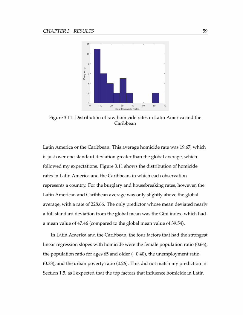
CHAPTER 3. RESULTS 59
Figure 3.11: Distribution of raw homicide rates in Latin America and theCaribbean
Latin America or the Caribbean. This average homicide rate was 19.67, which
is just over one standard deviation greater than the global average, which
followed my expectations. Figure 3.11 shows the distribution of homicide
rates in Latin America and the Caribbean, in which each observation
represents a country. For the burglary and housebreaking rates, however, the
Latin American and Caribbean average was only slightly above the global
average, with a rate of 228.66. The only predictor whose mean deviated nearly
a full standard deviation from the global mean was the Gini index, which had
a mean value of 47.46 (compared to the global mean value of 39.54).
In Latin America and the Caribbean, the four factors that had the strongest
linear regression slopes with homicide were the female population ratio (0.66),
the population ratio for ages 65 and older (−0.40), the unemployment ratio
(0.33), and the urban poverty ratio (0.26). This did not match my prediction in
Section 1.5, as I expected that the top factors that influence homicide in Latin

60 CHAPTER 3. RESULTS
America would be the government indicators. The four factors that had the
strongest slopes with burglary and housebreaking rates were GDP per capita
(2.66), Voice and Accountability (1.40), the female student ratio in primary
education (1.33), and the number of pure liters of alcohol consumed annually
per capita (1.20). Because only roughly half the countries in the dataset as a
whole had recorded burglary and housebreaking rates, they were only
available for 22 out of 33 of the countries in this region.
Europe
There were 47 European countries in the dataset. The average homicide rate
for these countries was 1.84, which is quite low, though not an entire standard
deviation below the worldwide mean. For the burglary and housebreaking
rates, the average across the European countries was 209.52, which is actually
slightly higher than the worldwide average. The factors whose means
deviated by at least one standard deviation (or very close to one standard
deviation) from the worldwide means can be found in Table 3.5.
In Europe, the factors that had the strongest linear regression slopes with
homicide were the adult literacy ratio (1.36), the female population ratio (0.81),
the population ratio for ages 0-14 (0.76), and Government Effectiveness
(−0.43). The factors that had the strongest slopes with burglary and
housebreaking rates were the adult literacy ratio (−1.74), the female student
ratio in primary education (1.03), the female student ratio in secondary
education (0.68), and the gross graduation ratio for secondary education (0.62).
These results suggest that education may play a large role in burglaries and

CHAPTER 3. RESULTS 61
Factor Europe Average Global Average
Gini index 31.72 39.54Gross enrollment ratio in secondary education 106.51 80.91
GDP per capita 79242 14520Annual pure liters of alcohol consumed per capita 9.48 4.98
Population ratio for ages 65 and older 16.58 8.38
Table 3.5: European means versus worldwide means of select factors
housebreakings in Europe. Burglary and housebreaking rates were available
for 41 out of the 47 European countries.
Africa
The Africa subset of the dataset included 53 countries, which is a larger
sample size than the previous two regions examined, but a large portion of
these countries were missing data for many of the factors. The average
homicide rate for the African countries was 7.99 per 100,000 population, which
is just marginally greater than the worldwide average of 7.66. The average
burglary and housebreaking rate in Africa was only 36.87, which is
significantly lower than the worldwide average. The factors whose means
deviated by at least one standard deviation (or very close to one standard
deviation) from the worldwide means can be found in Table 3.6. Notice that,
in general, many poverty-related factors in Africa had significantly higher
means and many education-related factors had significantly lower means than
those of the rest of the world.
In Africa, the factors that had the strongest slopes in a linear regression
with homicide were the population ratio for ages 65 and older (−0.49), GDP
per capita (−0.46), the Gini index (0.36), and the unemployment ratio (0.25).

62 CHAPTER 3. RESULTS
Factor Africa Average Global Average
Poverty ratio below $1.90 per day 37.43 19.27Poverty ratio below $3.10 per day 58.65 33.94
Poverty rate below the national poverty line 45.29 31.51Adult literacy ratio 67.70 84.18
Completion rate for primary education 73.39 89.76Gross enrollment ratio in secondary education 50.99 80.91Gross graduation ratio for secondary education 40.96 71.67
GDP per capita 2413 14520
Table 3.6: African means versus worldwide means of select factors
The factors that had the strongest slopes with burglary and housebreaking
rates were GDP per capita (3.68), the female population ratio (2.29), GDP per
capita growth (0.92), and the population ratio for ages 65 and older (0.75).
However, only 15 of the 53 had data available for burglary and housebreaking
rates, so these regression results are not particularly reliable.
Asia
There were 49 countries and two additional regions in China (Hong Kong and
Macau) included in the separate dataset for Asia. As was the case with Africa,
even though the dataset had more countries than those of Europe and Latin
America, a larger proportion of the countries were missing data for many of
the factors. The mean homicide rate in Asia was 4.48, which is lower than the
global mean, but still higher than Europe’s mean. The mean burglary and
housebreaking rate was 65.98, which is also lower than the global mean. The
only factor that was nearly a full standard deviation away from the worldwide
mean was the rural poverty ratio. The mean of this factor in Asian countries
was 23.82, which is much lower than the worldwide mean of 41.87.
The factors in Asia that had the steepest linear regression slopes with

CHAPTER 3. RESULTS 63
homicide were GDP per capita (−0.64), Control of Corruption (−0.64), Rule of
Law (−0.62), and Government Effectiveness (−0.57). These results are similar
to the worldwide homicide trends: three of the top four factors with the
strongest regression slopes were government indicators. The factors that had
the strongest slopes with burglary and housebreaking rates were the poverty
ratio below $1.90 per day (−1.74), the gross enrollment ratio in secondary
education (0.81), the rural poverty ratio (−0.81), and the poverty ratio below
$3.10 per day (−0.73). Notice that three of the factors with the highest
correlations with burglary and housebreaking in Asia were poverty-related.
Of the Asian regions and countries, 23 out of 51 had recorded burglary and
housebreaking rates.
3.5.3 Trends in Developing and Developed Countries
After I tested the four individual regions, to further observe the varying effects
of the attributes, I split the data into two categories: developing and
developed countries. Every country in the dataset was included in this portion
of the study.
Developing Countries
The United Nations Committee for Development Policy published a list of the
least developed countries around the world as of June 2017 [9]. I separated all
the countries on this list to analyze independently and assumed that all
countries not on the list are developed. There were 47 countries in total on the
list: 33 located in Africa, 9 in Asia, 4 in Oceania, and 1 in the Caribbean.

64 CHAPTER 3. RESULTS
Factor Developing Average Global Average
Poverty ratio below $1.90 per day 40.41 19.27Poverty ratio below $3.10 per day 63.55 33.94
Adult literacy ratio 61.72 84.18Completion rate for primary education 70.42 89.76
Gross enrollment ratio in secondary education 45.52 80.91Gross graduation ratio for secondary education 35.00 71.67
GDP per capita 1106 14520Population ratio for ages 0-14 40.57 28.11
Population ratio for ages 65 and older 3.39 8.38
Table 3.7: Developing country means versus worldwide means of select factors
The mean homicide rate in the 47 least developed countries was 7.70,
which is extremely close to the worldwide mean of 7.66, which suggests that
developing countries may not be inherently susceptible to higher rates of
homicide than other parts of the world. Homicide rates in these locations
tended to range from 1.8 to 14 cases per 100,000 population. Madagascar and
Burkina Faso were outliers on the low end of the spectrum with rates of 0.6
and 0.7, respectively, and Tuvalu and Lesotho were outliers on the high end of
the spectrum with rates of 20.3 and 38.0, respectively. Only 9 of the 47 least
developed countries had recorded burglary and housebreaking rates, so I only
analyzed homicide for this section of the analysis. A list of factors whose
means in developing countries deviated by at least one (or nearly one)
standard deviation from the worldwide means can be found in Table 3.7. Since
the majority of the developing countries were located in Africa, these results
are quite similar to those of Africa recorded in Table 3.6. Notice that a higher
portion of the population in these countries is younger than in other parts of
the world. There are generally fewer resources in these countries than in other
parts of the world, so it seems plausible that the age expectancy would be

CHAPTER 3. RESULTS 65
significantly lower. Additionally, as one might expect, the poverty ratios were
extremely high in these areas while the quality of education and GDP per
capita were fairly low.
The factors in the least developed countries that had the strongest linear
regression slopes with homicide were GDP per capita (2.54), the population
ratio for ages 65 and older (−0.68), the gross graduation ratio in secondary
education (−0.29), and Government Effectiveness (−0.28).
Developed Countries
I categorized the remaining 151 countries as developed, although I do
recognize that some of these countries are probably more developed than
others. The mean homicide rate of the developed countries was 7.68, which, as
was the case with the developing countries, is extremely close to the
worldwide mean. This matches our previous remark that a country’s
homicide rate may not be directly affected by whether or not it is developed.
Because roughly 75% of the countries were included in this category, none of
the factors differed significantly from the worldwide means. Since I was not
able to include burglary and housebreaking information in my analysis of the
least developed countries, I left it out of this section as well.
The four factors in the developed countries that had the strongest slopes in
linear regressions with homicide were the Gini index (0.69), the population
ratio for ages 0-14 (0.65), Government Effectiveness (−0.64), and Rule of Law
(−0.58). Notice that, as one might expect, these results are similar to those in
Section 3.2.1 regarding the worldwide linear regressions with homicide.

66 CHAPTER 3. RESULTS
3.6 Stepwise Regressions
There were many components to my code for the stepwise regression in
MATLAB. I did not want to perform the regression on all the factors in the
dataset at once for two reasons. First, all countries with missing data for any of
the predictors in the regression had to be removed for the regression to run
properly, and there were very few countries that had data available for every
factor, so the sample size in the regression would have been exceedingly small
if I had run all the factors at once. Secondly, I was concerned that considering
too many factors at once would confuse the stepwise regression and it would
therefore produce less accurate results. Thus, for the first round of stepwise
regressions that I ran, I split the data into categories and picked out the factors
that were selected often in these smaller categories.
As I previously mentioned, I did not run all the factors in a single stepwise
regression, so I split it into categories, ran the regression multiple times for
each category, and then combined all the factors from each category that were
regularly selected. The categories that I split my data into were: poverty and
income inequality, education, governance indicators, ethno-linguistic and
religious indices, and other. After I divided the data into categories, I built a
loop to temporarily remove every country that had data missing for any of the
factors under consideration. Next, I randomly split the remaining data into
training and testing data at a 4:1 ratio. I used MATLAB’s stepwiseglm
command to run a stepwise regression on the factors, with a p-value of 0.1
necessary to be added to the model and a p-value of 0.15 necessary to be
removed. For every factor that I added, I calculated the model’s mean square

CHAPTER 3. RESULTS 67
error with cross-validation using MATLAB’s cvMSE command with the
number of folds set to 5. I arbitrarily chose to have 5 folds because I felt that it
was enough to sufficiently evaluate the data without splitting it up too much.
It also followed the 4:1 training to testing ratio that I used throughput this
study. My code then continued adding and removing factors and running the
cross-validation error calculation until there were no more factors to add to the
model. The cross-validation recorded the model error with cross-validation as
each factor was added. If the cross validation error increased as factors were
added, then the factors were probably overfitting with one another.
I ran the stepwise regression with these chosen factors numerous times
and took note of the different combinations of factors that were selected
together. I eventually tested all of these final combinations (more details on
this process will be provided in the next section). The full list of predictors that
I selected to be evaluated in the final stepwise regressions for both of the
crimes can be found in the Appendix.
Often, I found that different combinations of factors were selected by the
stepwise regression with homicide on separate runs of my code. I made a note
of every combination to be modeled later, but there were some combinations
that were selected more often than others. The combinations of factors that
were selected three or more times for homicide can also be found in the
Appendix. Even though different combinations were often selected, I noticed
that there were some factors that were selected often and others that were
almost never selected.
However, the stepwise regression with burglary and housebreaking rates
very rarely produced duplicate factor combinations: almost every regression

68 CHAPTER 3. RESULTS
produced a combination that I had not previously seen. Additionally, it was
much more difficult to pick out factors that were selected regularly because
the selection of factors seemed much more erratic. This may have been due to
the smaller sample size.
3.7 Final Models
To build final models for aggregated crime rates around the world, I created
models for every factor combination yielded by the stepwise regressions
(detailed in Section 3.6) to observe which combinations produced the lowest
mean absolute error value. I built two different models for each combination:
a random forest of regression trees and a generalized linear model (the
methodology of these techniques is detailed in Sections 2.8 and 2.9,
respectively). To test the models, I randomly separated 80% of the data
observations to be included in the training dataset, built a model to that, and
tested the predictability of the model on the remaining 20% (the testing set). I
then found the average crime rate of the testing data to use as a baseline model
and compared the mean absolute error of the baseline model tho that of the
random forest model and generalized linear model (when applied to the
testing data). I considered the most successful model to be that which had the
largest error reduction from that of the baseline.
Because the mean absolute error of the models depended heavily on
exactly how the data was separated into the training and testing sets, I made a
loop that built 200 models for each combination of factors, with each loop
randomly partitioning the data into training and testing, building a model

CHAPTER 3. RESULTS 69
from the training data, applying that model to the testing data, finding the
baseline value of the testing data, and calculating the mean absolute error of
my model. I then averaged the error values over the 200 loops. I also averaged
the baseline model’s mean absolute error values over the loops. I arbitrarily
selected 200 as the number of loops because I felt that it was a large enough
number to produce reliable error results without being so large that it
substantially slowed the program. I compared the average error of my models
to the average error of the baseline models so that I could observe how the
accuracy of my model compared to that of the baseline over the 200 loops. I
also averaged the linear model coefficients of the predictors in both models at
each loop.
To create a random forest of regression trees in MATLAB, I used the
TreeBagger command with the training observations of the factors I wanted to
model and the crime rates, the number of regression trees I wanted in each
forest (I arbitrarily chose 10 for this analysis), and the keyword ‘regression’ as
parameters. This built a random forest from the testing data, from which I
then built a model using the testing observations of the factors with the predict
command.
To find generalized linear model coefficients in MATLAB, I used the glmfit
command with the training observations of the factors that I wanted to model
together, the crime rates, and the desired model fit (for my models, I used the
keyword ’normal’ to indicate that I wanted to use the linear regression model)
as parameters. I then used the glmval command with the testing observations
of the factors and the model coefficients that I had found to generate model
prediction values.

70 CHAPTER 3. RESULTS
3.7.1 Homicide Model
To model worldwide homicide rates, the combination of factors that generated
the largest mean absolute error reduction from the baseline model was: the
Gini index, Rule of Law, the unemployment ratio, and the binomial variable
indicating whether or not a country is located in Latin America. With mean
absolute error values averaged over 200 loops, the generalized linear model
with these factors had approximately 38.5% less error than the baseline. For
almost every combination of factors that I tested, the generalized linear
models produced less error than the random forest modeling technique.
We saw that countries in Latin America and the Caribbean do, indeed,
tend to have higher average homicide rates than other parts of the world, so it
is not surprising that it was included in the final aggregate homicide model.
Additionally, we showed in Section 3.2.1 that the Gini index and Rule of Law
both had strong correlations with homicide, so it was also expected that they
would be included in the model. The unemployment ratio did not have a
particularly strong correlation, so its inclusion in the model was more
unexpected. The list of average model coefficients is shown in Table 3.8.
Factor Average Model Coefficient
Rule of Law −0.40Gini index 0.32
Latin America binomial indicator 0.30Unemployment ratio 0.07
Constant Term 0.04
Table 3.8: Generalized linear model coefficients for the homicide model

CHAPTER 3. RESULTS 71
3.7.2 Burglary and Housebreaking Model
To model worldwide burglary and housebreaking rates, the combination of
factors that generated the largest mean absolute error reduction from the
baseline model was: Voice and Accountability, the gross enrollment ratio in
secondary education, Regulatory Quality, and Control of Corruption. The
generalized linear model with these factors had approximately 31% less error
than the baseline. As with the homicide model, the generalized linear models
usually had lower error values than the random forest technique for most
combinations of factors.
It was not surprising that the gross enrollment ratio was included in this
model, as it was the factor that had the highest correlation with burglary and
housebreaking. It was unexpected, however, that the other factors were all
government indicators, as Voice and Accountability was the only indicator
that had a strong linear regression slope with burglary and housebreaking
rates. Additionally, there may have been some overfitting among the three
governance indicators, but the cross validation mean square error did not
increase as any of these indicators were added to the model, so I decided it
was appropriate to include them all together. The list of average model
coefficients is shown in Table 3.9.
Factor Average Model Coefficient
Voice and Accountability 0.46Gross enrollment ratio in secondary education 0.42
Control of Corruption 0.29Regulatory Quality −0.28
Constant Term −0.30
Table 3.9: Generalized linear model coefficients for the burglary andhousebreaking model

72 CHAPTER 3. RESULTS

Chapter 4
Discussion
This chapter concludes my crime modeling study by reviewing and
interpreting the results found in the previous chapter, discussing the flaws of
the final crime models, and examining future research opportunities that
follow this analysis.
4.1 Modeling Results
In Chapter 1, I initially predicted, based on literature, that worldwide crime
would be influenced by economic indicators (specifically poverty and income
inequality), education rates, government indicators, ethno-linguistic
fractionalization, GDP per capita and its growth, drug consumption rates, and
age and gender ratios. I found that some of these factors did, indeed, come into
play for both aggregate homicide rates and burglary and housebreaking rates,
although various factors affected the two crimes differently. In fact, the crimes
actually seemed to have opposite correlations with most of the predictors.
73

74 CHAPTER 4. DISCUSSION
I found that, when performing linear regressions with the predictors and
crime rates in individual regions around the world, some predictors repeatedly
generated strong slopes in different regions. These factors included the gross
enrollment and graduation ratios in secondary education, the government
indicators, GDP per capita, and the population and gender ratios. However,
when building the final aggregate models, neither GDP per capita nor the
population and gender ratios were included in either crime’s model. It could
therefore be possible that these factors have a high correlation with crime rates
regionally, but they lose some of that significance at a worldwide level.
4.1.1 Homicide Model
The Gini index had the strongest linear regression slope with homicide. It was
also included in the final homicide generalized linear model. This suggests
that income inequality may, indeed, be a driving factor in many homicides
around the world. Interestingly enough, the Gini index did not have a strong
correlation with homicide in any of the regions examined individually (Latin
America and the Caribbean, Europe, Africa, and Asia)–it only seemed to be
significant at a worldwide level.
The government indicators seemed to have a high correlation with
homicide rates both globally and regionally. The government indicators that
had notably strong linear regression slopes with homicide were Government
Effectiveness, Rule of Law, Regulatory Quality, and Control of Corruption. Of
these, only Rule of Law was included in the final homicide model, but this was
the factor with the strongest model coefficient, which tells us that it was the

CHAPTER 4. DISCUSSION 75
driving factor in the model.
The unemployment rate was included in the homicide model, but it did
not have a significant linear regression slope with homicide, nor did it have a
high model coefficient. It was often selected by the stepwise regression along
with the Gini index, though, and its inclusion in the model slightly reduced its
mean absolute error, so I elected to use it.
The binomial indicator regarding whether a country is located in Latin
America or the Caribbean was also used in the homicide model, and it had a
reasonably high model coefficient, which means that the model automatically
predicts that a country in this region will have a higher homicide rate than it
otherwise would have if it was located in another part of the world. This is in
accordance with the results in Section 3.5.2 that showed that the mean
homicide rate in Latin America and the Caribbean is a full standard deviation
higher than that of the rest of the world.
4.1.2 Burglary and Housebreaking Model
The gross enrollment ratio in secondary education had the strongest linear
regression slope with the burglary and housebreaking rates, and it was,
unsurprisingly, included in the burglary and housebreaking model. In fact,
most of the factors relating to education seemed to have a heavier impact on
burglary and housebreaking than they did on homicide.
The other three factors that were included in the burglary and
housebreaking model were all government indicators: Voice and
Accountability, Control of Corruption, and Regulatory Quality. Note that

76 CHAPTER 4. DISCUSSION
these government indicators all came from separate categories of government
quality (refer to Section 1.3 for more details). It is possible, or perhaps likely,
that overfitting occurred between these factors in the final model, but
combinations of these factors were frequently selected together in the stepwise
regression, and since the cross-validation mean square error did not increase
when the factors were used together, I allowed them all to be used in the same
model.
4.2 Link Between Property Crime and Homicide
This study did not find a strong positive correlation between homicide and
burglary and housebreaking; on the contrary, it found a slightly negative
correlation between the two. This was quite unexpected, as one might predict
that countries with higher homicide rates would have higher property crime
rates and vice versa. In fact, literature regarding the relationship between
violent and property crime indicated that there should have been a positive
relationship between the crime rates in this analysis. Previous crime analyses
have found significant positive correlations between homicide and property
crime [39].
Studies have found that property crime and homicide tend to have similar
trends over time. This means that as one increases, the other is likely to follow
suit, and vice versa [39]. This is often due, in part, to a country’s changing
economic conditions: as the economy worsens, both types of crime are likely
to fluctuate along with it [39]. This was not surprising, as this study did find a
relationship between economic conditions (specifically poverty and income

CHAPTER 4. DISCUSSION 77
inequality) and both forms of crime.
In addition to economic conditions, there is usually a correlation between
property crime and violent crime because, in many cases, involvement in
property crime directly results in involvement in violent crime [39]. For
example, if a burglar is caught breaking and entering in someone’s home, the
victim may react by attacking, or even killing, the perpetrator as an act of
self-defense. Thus, the two forms of crime have the potential be directly
connected with each other, which does lead one to suspect that an increase in
one could provoke an increase in the other.
This study found a slight negative correlation between homicide rates and
burglary and housebreaking rates, which begs the question: was there
something wrong with the data?
4.2.1 Burglary and Housebreaking Data Irregularities
A possible explanation for the unexpected correlation between worldwide
homicide rates and burglary and housebreaking rates could be attributed to a
lack of reporting of burglary and housebreaking, both by victims and police
departments.
When a homicide is committed, it is almost always reported, as it is
probably quite difficult to ignore. In most parts of the world, instances of
homicide are taken seriously, so the majority of police departments around the
world probably have reasonably reliable homicide records. However, this may
not be the case with burglary and housebreaking rates. Police departments
may not be as meticulous with their property crime records as they are with

78 CHAPTER 4. DISCUSSION
their homicide records, so the rates reported by a country may not be an
accurate representation of its actual frequency of property crime occurrences.
Additionally, many victims of burglary and housebreaking may not feel the
need to report the crime if they feel that the crime was not particularly severe:
they may fear that it would be a waste of police time. Thus, these incidences
would also go unrecorded.
Police Misreporting of Property Crime
The police departments of different countries around the world may have
different levels of attentiveness when it comes to recording and reporting
burglary and housebreaking rates. It has been shown that a large amount of
measurement error can be found in many forms of property crime data,
mainly relating to differences in police jurisdictions and reporting practices as
well as technological variations in crime reporting around the world [34].
Studies have found that property crimes are more likely to be reported if
there is a larger and more reliable police department [34]. A stronger police
department is often correlated with lower homicide rates, as people are less
likely to commit violent crimes if there is a higher chance that they get caught
and punished. However, there tend to be more reported incidences of
property crimes in areas with stronger police departments [34]. This could be
due to an increase in reporting of these crimes rather than an actual increase in
the frequency of the crimes, especially considering the fact that homicide rates
decrease under the same circumstances [34].
Additionally, stronger police forces may have the extra manpower that

CHAPTER 4. DISCUSSION 79
allows them to be more careful in their reporting of property crimes [34]. If
there are two locations with perfectly equal amounts of crime, but different
amounts of manpower in their respective police departments, the location
with the larger police department may report more property crimes, as they
have the extra manpower to put in the time to record every crime, even the
minor ones. However, because homicide is taken more seriously in most parts
of the world, even the smaller police departments are probably fairly diligent
with their homicide records.
Victim Misreporting of Property Crime
The possible lack of property crime reporting may not be solely the fault of
police departments: some victims of burglary and housebreaking may not feel
the need to report an incident, and if the victim does not file a report, then it
will not go on record.
There are many reasons for which a burglary or housebreaking victim
might not inform the police of the crime. The victim may feel that the costs
outweigh the benefits of reporting the crime–they might think that the
inconvenience would not be worth it, as they could be forced to go to the
police station, or even court, in the process. They might not want their friends
and neighbors to find out that they were robbed, as that might cause them to
feel embarrassed or vulnerable. They might also fear that the crime was so
minor that a report would be a waste of time for all parties involved [41]. They
also might suspect that there is a small likelihood that the crime would be
solved, even if it was reported, and that reporting it would just create an

80 CHAPTER 4. DISCUSSION
unnecessary hassle [41]. Studies have found that victims of property crime
that have higher incomes and levels of educational attainment are more likely
than others to report an incident [41]. This could be, in part, because people
with higher incomes may have more to gain by reporting the crime, even
taking into consideration the costs incurred in the process.
However, some victims may not want to report an instance of property
crime for reasons that are rooted in the quality of their local police department.
First, as mentioned before, someone may not want to report a crime if they feel
that it has a low chance of being solved. A low amount of manpower on the
local police force could hamper the chances of catching the perpetrator, thus
making any reports of minor crimes seem futile. It has also been found that
people who hold the police in higher regards are more likely to report minor
crimes like burglary and housebreaking [41]. Hence, if the victim of property
crime feels that they have a poor local police force, then they may have a more
negative opinion about the police and therefore wish to avoid them.
Quality of Governance and Property Crime
It seems reasonable to suspect that countries with overall better governments
may have higher quality police forces (with generally more manpower). In
particular, countries with strong governments may have more money to
allocate to their nations’ police departments.
The homicide rates had, for the most part, the relationships with the
factors that were predicted in Chapter 1, but the burglary and housebreaking
rates did not. This study found strong positive correlations between

CHAPTER 4. DISCUSSION 81
government quality ratings and burglary and housebreaking rates: countries
with better governments actually have more reported instances of burglary
and housebreaking. While, at first glance, this does appear counter-intuitive,
when observed from a different angle, it seems plausible that the ideas
discussed in this section came into play in the burglary and housebreaking
data used in this study. It is possible that countries with stronger governments
have stronger police forces, which could lead to an increased percentage of
minor property crimes being reported.
These ideas are one possible interpretation of the unexpected correlations
found by this study between most of the predictors and burglary and
housebreaking rates, but they are, by no means, guaranteed to be the only
definitive answer. It should also be noted that the government indicator that
measured the respect of the general population for the police (among other
things) was Rule of Law, which had a strong correlation with homicide, but
not with burglary and housebreaking.
4.3 Flaws in the Final Models
There were some flaws in the data and modeling techniques used in this study
that may have inhibited the success of the final models.
As one will find in any analytical study, there was noise in the data that the
models were unable to predict. We saw this particularly in the case of the
burglary and housebreaking model, as these crime rates were particularly
erratic. It is possible that some of the other data factors had similar noise
levels. Next, as detailed in Section 3.1.1, the data in this study was aggregated

82 CHAPTER 4. DISCUSSION
and each country’s data was given by the most recent recorded value for each
factor, which means that different factors were composed of values from
different years for some countries. It is also probable that many of these factors
are highly dependent on one another, even if they belong to different
categories, so even though precautions were put in place to avoid overfitting
(such as cross-validation and the separation of data into testing and training
sets), it still may have occurred to some degree. Finally, none of the factors or
crime rates had perfectly normal distributions, and the generalized linear
models used for the final models assumes normality for all the data.
There were also flaws in the modeling techniques that may have affected
the models’ accuracy. First, researching machine learning techniques beyond
random forests may have allowed me to find a model that was both more
accurate than the generalized linear models and did not assume normality for
all the factors. Additionally, exploring more methods of data transformation
may have helped me alter certain factors so that they were more normal and
had stronger linear regression slopes with the crime rates, as the logarithmic
transformation did not yield successful results for all the factors tested (further
details of the data transformation process can be found in Section 3.3).
4.4 Future Work
This study pinpointed factors that appear to influence crime rates around the
world, whether positively or negatively. The data used in this analysis,
however, was aggregated and only available on a country-wide level. An
interesting next step could be to examine more specific data centered on

CHAPTER 4. DISCUSSION 83
individual countries and observe which factors appear to affect crime in
individual countries (rather than on a worldwide level).
Further work on this analysis could also involve modeling crime rates in
different regions around the world. While this study did take into account
linear regressions and mean values of all the factors for multiple regions and
developing countries, looking more closely at these regions and actually
modeling location-specific crime rates could have been a next step to
understanding what influences crime around the world.
Another direction that could have been taken if this study were to be
continued would be to analyze more varieties of crime. This study only
considered homicide rates and burglary and housebreaking rates, but there are
more types of crime that could be interesting to examine, such as assault or
kidnapping. Modeling homicide rates with and without firearms to see
whether there is a trend in which people may be more likely to use guns as a
primary murder weapon could also be a next step.

84 CHAPTER 4. DISCUSSION

Appendix A
Tables and Lists
This section contains tables and lists referenced throughout Chapter 3.
The list of factors considered in the final stepwise regressions with the
homicide data were:
1. The unemployment ratio
2. The rural poverty ratio
3. The poverty ratio below $3.10 per day
4. The Gini index
5. Expenditure on education as a share of GNI
6. The gross enrollment ratio in primary education
7. The gross enrollment ratio in secondary education
8. The gross graduation ratio for secondary education
9. The female student ratio in primary education
85

86 APPENDIX A. TABLES AND LISTS
10. Voice and Accountability
11. Rule of Law
12. Ethnic index
13. Language index
14. ELF index
15. GDP per capita
16. GDP per capita growth
17. Liters of alcohol consumed annually per capita
18. The population ratio for ages 65 and older
19. The female population ratio
20. The binomial Latin America and Caribbean indicator
Of these factors, the combinations that were selected three or more times by
the stepwise regression were:
1. The unemployment ratio, the rural poverty ratio, and the gross
enrollment ratio in primary education
2. The Gini index and the gross enrollment ratio in primary education
3. The Gini index, the gross enrollment ratio in primary education, and the
binomial Latin America and Caribbean indicator
4. The Gini index, Rule of Law, the unemployment ratio, and the binomial
Latin America and Caribbean indicator

APPENDIX A. TABLES AND LISTS 87
The list of factors considered in the final stepwise regression with the
burglary and housebreaking data were:
1. The unemployment ratio
2. The poverty ratio below $3.10 per day
3. The urban poverty ratio
4. The rural poverty ratio
5. Expenditure on education as a share of GNI
6. The gross enrollment ratio in primary education
7. The gross enrollment ratio in secondary education
8. The gross graduation ratio in secondary education
9. The female student ratio in secondary education
10. Voice and Accountability
11. Regulatory Quality
12. Control of Corruption
13. Ethnic index
14. GDP per capita
15. The population ratio for ages 65 and older
16. The female population ratio
17. The PCA of drug consumption rates (illustrated in Table 3.4)

88 APPENDIX A. TABLES AND LISTS
Factor Linear Regression Slope
Gini Index 0.61Government Effectiveness −0.54
Rule of Law −0.53Regulatory Quality −0.49
Control of Corruption −0.47Population ratio for ages 65 and older −0.47
Population ratio for ages 0-14 0.45GDP per capita −0.40
Gross enrollment ratio in secondary education −0.35Political Stability −0.33
Gross graduation ratio in secondary education −0.33ELF index 0.31
Rural poverty ratio 0.30Completion ratio for primary education −0.28
Poverty ratio below the national poverty line 0.27Ethnic index 0.26
Public expenditure on education 0.25Unemployment ratio 0.23
Voice and Accountability −0.23Urban poverty ratio 0.22
GDP per capita growth −0.22Adult literacy ratio −0.21
Liters of alcohol consumed annually per capita −0.18Female student ratio in primary education −0.16
Percent of population that admitted to consuming cannabis −0.15Language index 0.13
Poverty ratio below $3.10 per day 0.13Poverty ratio below $1.90 per day 0.12
Female population ratio 0.10Gross enrollment ratio in primary education −0.05Female student ratio in secondary education −0.05
Religious index 0.05Expenditure on education as a share of GNI 0.01
Table A.1: Linear regression slope of with homicide for each factor

APPENDIX A. TABLES AND LISTS 89
Factor Linear Regression Slope
Gross enrollment ratio in secondary education 0.79Voice and Accountability 0.74
Poverty ratio below $1.90 per day −0.74Female enrollment ratio in primary education 0.73
Gross graduation ratio for secondary education 0.66Adult literacy ratio 0.64
Female enrollment ratio in secondary education 0.62Poverty ratio below $3.10 per day −0.62
Population ratio for ages 0-14 −0.62Rule of Law 0.61
Control of Corruption 0.58Government Effectiveness 0.58
Regulatory Quality 0.58Liters of alcohol consumed annually per capita 0.56
Political Stability 0.56Population ratio for ages 65 and older 0.52
Expenditure on education as a share of GNI 0.52Rural poverty ratio −0.50
Poverty ratio below the national poverty line −0.48Ethnic index −0.45
Language index −0.39GDP per capita 0.37
Urban poverty ratio −0.36Completion ratio for primary education 0.32
Percent of population that admitted to consuming cannabis 0.31ELF index −0.29Gini index −0.24
GDP per capita growth 0.20Female population ratio 0.15
Unemployment ratio 0.15Religious index 0.12
Public expenditure on education −0.10Gross enrollment ratio in primary education −0.04
Table A.2: Linear regression slope of with burglary and housebreaking foreach factor
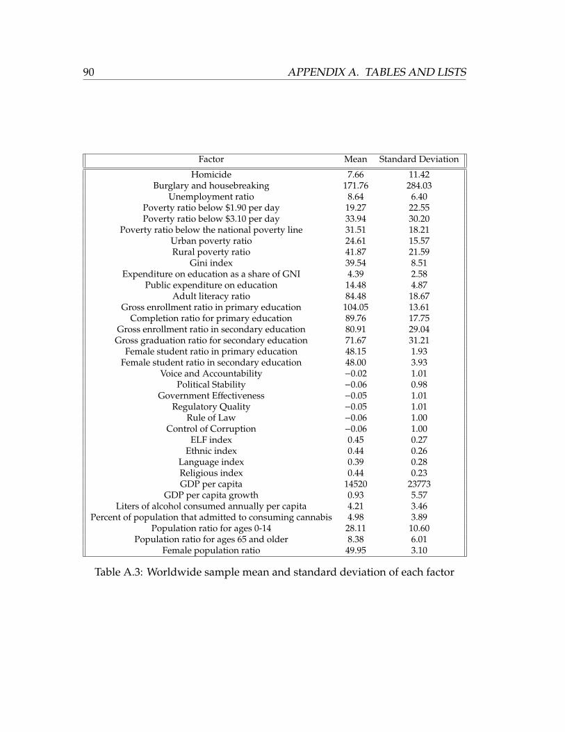
90 APPENDIX A. TABLES AND LISTS
Factor Mean Standard Deviation
Homicide 7.66 11.42Burglary and housebreaking 171.76 284.03
Unemployment ratio 8.64 6.40Poverty ratio below $1.90 per day 19.27 22.55Poverty ratio below $3.10 per day 33.94 30.20
Poverty ratio below the national poverty line 31.51 18.21Urban poverty ratio 24.61 15.57Rural poverty ratio 41.87 21.59
Gini index 39.54 8.51Expenditure on education as a share of GNI 4.39 2.58
Public expenditure on education 14.48 4.87Adult literacy ratio 84.48 18.67
Gross enrollment ratio in primary education 104.05 13.61Completion ratio for primary education 89.76 17.75
Gross enrollment ratio in secondary education 80.91 29.04Gross graduation ratio for secondary education 71.67 31.21
Female student ratio in primary education 48.15 1.93Female student ratio in secondary education 48.00 3.93
Voice and Accountability −0.02 1.01Political Stability −0.06 0.98
Government Effectiveness −0.05 1.01Regulatory Quality −0.05 1.01
Rule of Law −0.06 1.00Control of Corruption −0.06 1.00
ELF index 0.45 0.27Ethnic index 0.44 0.26
Language index 0.39 0.28Religious index 0.44 0.23GDP per capita 14520 23773
GDP per capita growth 0.93 5.57Liters of alcohol consumed annually per capita 4.21 3.46
Percent of population that admitted to consuming cannabis 4.98 3.89Population ratio for ages 0-14 28.11 10.60
Population ratio for ages 65 and older 8.38 6.01Female population ratio 49.95 3.10
Table A.3: Worldwide sample mean and standard deviation of each factor

Bibliography
[1] 6.1–Introduction to Generalized Linear Models.
https://onlinecourses.science.psu.edu/stat504/node/216.
[2] Confidence Interval. http://stattrek.com/statistics/dictionary.
aspx?definition=confidence%20interval.
[3] Finding Eigenvalues and Eigenvectors.
https://www.scss.tcd.ie/˜dahyotr/CS1BA1/SolutionEigen.pdf.
[4] Gender and Crime - Differences Between Male And Female Offending
Patterns. http://law.jrank.org/pages/1250/
Gender-Crime-Differences-between-male-female-offending-patterns.
html.
[5] Gini coefficient. http://www3.nccu.edu.tw/˜jthuang/Gini.pdf.
[6] Gini coefficient. https://en.wikipedia.org/wiki/Gini_coefficient.
[7] Interpreting residual plots to improve your regression.
http://docs.statwing.com/
91

92 BIBLIOGRAPHY
interpreting-residual-plots-to-improve-your-regression/
#large-axis-header.
[8] Latin America and the Caribbean. http://www.unesco.org/new/en/
unesco/worldwide/latin-america-and-the-caribbean/.
[9] List of Least Developed Countries (as of June 2017).
https://www.un.org/development/desa/dpad/wp-content/uploads/
sites/45/publication/ldc_list.pdf.
[10] Mean Vector and Covariance Matrix. http:
//www.itl.nist.gov/div898/handbook/pmc/section5/pmc541.htm.
[11] Multiple linear regression.
http://www.stat.yale.edu/Courses/1997-98/101/linmult.htm.
[12] Normal Distributions: Definition, Word Problems.
http://www.statisticshowto.com/probability-and-statistics/
normal-distributions/.
[13] Regression Trees. https://www.solver.com/regression-trees.
[14] zscore. https://www.mathworks.com/help/stats/zscore.html.
[15] Prevalence of drug use in the general population - national data .
https://www.unodc.org/wdr2017/en/maps-and-graphs.html,
2001-2017.
[16] Recorded alcohol per capita consumption, from 2000, Last update: May
2016. http://apps.who.int/gho/data/node.main.A1026?lang=en?
showonly=GISAH, 2011.

BIBLIOGRAPHY 93
[17] World Data Atlas. https://knoema.com/atlas, 2011.
[18] A Complete Tutorial on Tree Based Modeling from Scratch (in R and
Python). https://www.analyticsvidhya.com/blog/2016/04/
complete-tutorial-tree-based-modeling-scratch-in-python/, 2016.
[19] Miller Analogies Test Bell Curve.
https://magoosh.com/mat/miller-analogies-test-bell-curve/,
May 2016.
[20] 10.2 - stepwise regression.
https://onlinecourses.science.psu.edu/stat501/node/329, 2017.
[21] 3.1 Cross-validation: evaluating estimator performance.
http://scikit-learn.org/stable/modules/cross_validation.html,
2017.
[22] Alberto Alesina, Arnaud Devleeschauwer, William Easterly, Sergio
Kurlat, and Romain Wacziarg. Fractionalization. The National Bureau of
Economic Research Working Paper, (9411), January 2003.
[23] Blaine Robbins and David Pettinicchio. Social Capital, Economic
Development, and Homicide: A Cross-National Investigation. Social
Indicators Research, 105(3):519–540, February 2012.
[24] Richard H. Blum. Drugs, Behavior, and Crime. The Annals of the American
Academy of Political and Social Science, 374:135–146, November 1967.
[25] Jason Brownlee. Bagging and Random Forest Ensemble Al-
gorithms for Machine Learning. https://machinelearningmastery.com/

94 BIBLIOGRAPHY
bagging-and-random-forest-ensemble-algorithms-for-machine-learning/,
2016.
[26] Francesco Caselli and Wilbur John Coleman II. On the Theory of Ethnic
Conflict. National Bureau of Economic Research, (12125), March 2006.
[27] Julio H. Cole and Andrs Marroqun Gramajo. Homicide Rates in a
Cross-Section of Countries: Evidence and Interpretations. Population and
Development Review, 35(4):749–776, December 2009.
[28] Lee Ellis and James N. McDonald. Crime, Delinquency, and Social Status.
Journal of Offender Rehabilitation, 32:23–52, January 2001.
[29] Pablo Fajnzylber, Daniel Lederman, and Norman Loayza. Inequality and
Violent Crime. The Journal of Law & Economics, 45(1):1–39, April 2002.
[30] Jake Hoare. Machine Learning: Pruning Decision Trees. https:
//www.displayr.com/machine-learning-pruning-decision-trees/,
2017.
[31] Daniel Kaufmann, Aart Kraay, and Massimo Mastruzzi. The Worldwide
Governance Indicators: Methodology and Analytical Issues. World Bank
Policy Research Working Paper, 5430, September 2010.
[32] Morgan Kelly. Inequality and Crime. The Review of Economics and
Statistics, 82(4):530–539, November 2000.
[33] M.A. Khamsi. Determinants of Matrices of Higher Order.
http://www.sosmath.com/matrix/determ1/determ1.html.

BIBLIOGRAPHY 95
[34] Steven D. Levitt. The Relationship Between Crime Reporting and Police:
Implications for the Use of Uniform Crime Reports. Journal of Quantitative
Criminology, 14(1):61–81, 1998.
[35] Stephen Machin, Olivier Marie, and Sunica Vuji. The Crime Reducing
Effect of Education. The Economic Journal, 121(552):463–484, May 2011.
[36] Magaly Sanchez. Insecurity and Poverty as a New Power Relation in
Latin America. The Annals of the American Academy of Political and Social
Science, 606:178–195, July 2006.
[37] Sebastian Raschka. Principal Component Analysis in 3 Simple Steps.
http://sebastianraschka.com/Articles/2015_pca_in_3_steps.html,
January 2015.
[38] Philip G. Roeder. Ethnolinguistic Fractionalization (ELF) Indices, 1961
and 1985. http://pages.ucsd.edu/˜proeder/elf.htm, February 2001.
[39] Richard Rosendeld. Crime is the Problem: Homicide, Acquisitive Crime,
and Economic Conditions. Journal of Quantitative Criminology,
25(3):287–306, May 2009.
[40] Patrick Sharkey, Max Besbris, and Michael Friedson. Poverty and Crime.
The Oxford Handbook of the Social Science of Poverty, May 2016.
[41] Roger Tarling and Katie Morris. Reporting Crime to the Police. The British
Journal of Criminology, 50(3):474–490, May 2010.
[42] William M.K. Trochim. The T-Test.
https://www.socialresearchmethods.net/kb/stat_t.php, 2006.

96 BIBLIOGRAPHY
[43] Jeffery T. Ulmer and Darrell Steffensmeier. The Age and Crime
Relationship: Social Variation, Social Explanations. In The Nurture Versus
Biosocial Debate in Criminology: On the Origins of Criminal Behavior and
Criminality, pages 377–396. SAGE Publications, London, 2014.
[44] Eric W. Weisstein. Covariance.
http://mathworld.wolfram.com/Covariance.html.

![Mathematical Olympiads - Problems and Solutions From Around the World [2000-2001] - T. Andreescu, Z. Feng WW](https://img.pdfslide.us/doc/110x75/557213a6497959fc0b92ba7a/mathematical-olympiads-problems-and-solutions-from-around-the-world-2000-2001.jpg)


![[Math] Mathematical Olympiad Problems From Around the World 2](https://img.pdfslide.us/doc/110x75/54f7f4604a79590a4e8b477e/math-mathematical-olympiad-problems-from-around-the-world-2.jpg)