creta Monthly GDP

1E U R O P E A NC O M M I S S I O N

THEME 1Generalstatistics

A Monthly Indicator of GDP for the Euro-zone

16

2

00

1

A great deal of additional information on the European Union is available on the Internet.It can be accessed through the Europa server (http://europa.eu.int).

Luxembourg: Office for Official Publications of the European Communities, 2001

© European Communities, 2001

Printed in Belgium

PRINTED ON WHITE CHLORINE-FREE PAPER

INDEX

1. Introduction . . . . . . . . . . . . . . . . . . . . . . . . . . . . . . . . . . . . . . . . . . . . . . . . . . . . . . . . . . . . . . . . . . . . . . . . . . . . . . . 1

2. The methodology. . . . . . . . . . . . . . . . . . . . . . . . . . . . . . . . . . . . . . . . . . . . . . . . . . . . . . . . . . . . . . . . . . . . . . . . . . 23. Estimation of monthly GDP . . . . . . . . . . . . . . . . . . . . . . . . . . . . . . . . . . . . . . . . . . . . . . . . . . . . . . . . . . . . . . . 5

3.1. Data availability. . . . . . . . . . . . . . . . . . . . . . . . . . . . . . . . . . . . . . . . . . . . . . . . . . . . . . . . . . . . . . . . . . . . . . 53.2. Estimation . . . . . . . . . . . . . . . . . . . . . . . . . . . . . . . . . . . . . . . . . . . . . . . . . . . . . . . . . . . . . . . . . . . . . . . . . . . 63.3. An alternative approach . . . . . . . . . . . . . . . . . . . . . . . . . . . . . . . . . . . . . . . . . . . . . . . . . . . . . . . . . . . . . . 8

4. Conclusions . . . . . . . . . . . . . . . . . . . . . . . . . . . . . . . . . . . . . . . . . . . . . . . . . . . . . . . . . . . . . . . . . . . . . . . . . . . . . . . 10

References. . . . . . . . . . . . . . . . . . . . . . . . . . . . . . . . . . . . . . . . . . . . . . . . . . . . . . . . . . . . . . . . . . . . . . . . . . . . . . . . . . . . 10

$�0RQWKO\�,QGLFDWRU�RI�*'3�IRU�WKH�(XUR�]RQH

Roberto ASTOLFI Dominique LADIRAY�6'$�6WDWLVWLFDO�6WXGLHV�DQG�'DWD�$QDO\VLV (XURVWDW��$��5XH�GHV�%DLQV��/��/X[HPERXUJ -HDQ�0RQQHW�%XLOGLQJ��/��/X[HPERXUJH�PDLO�UREHUWR�DVWROIL#SODQLVWDW�OX H�PDLO�GRPLQLTXH�ODGLUD\#FHF�HX�LQW

Gian Luigi MAZZI Fabio SARTORI(XURVWDW��$� (XURVWDW��$�

H�PDLO�JLDQOXLJL�PD]]L#FHF�HX�LQW H�PDLO�IDELR�VDUWRUL#FHF�HX�LQW

Regina SOARES(XURVWDW��$�

H�PDLO�UHJLQD�VRDUHV#FHF�HX�LQW

�� ,QWURGXFWLRQ

In the last few years the interest in short-term statistics has considerably increased. Theavailability of statistics suitable to give an image of the economy with a short delay and ina reliable way has become one of the main challenges for Eurostat. This attitude justifies,for example, the increasing role played by quarterly national accounts, which give acomplete and coherent picture of the economic situation.

In addition to quarterly accounts several monthly statistics are currently available supplyingindications of short-term movements in demand, output, prices and wages. Despite of theirearly availability and higher frequency, these statistics provide only a partial and thusincomplete picture of the economy.

It is well known that the capability of identifying correctly the short-term pattern of aneconomic phenomenon increases with the frequency of the observations. On the other hand,a higher frequency is often associated with a higher volatility in the series; this is

5�$VWROIL��'�/DGLUD\��*�/�0D]]L��)�6DUWRUL��5�6RDUHV

2

considered the most important limit to the use of high frequency data.

The project of deriving a monthly indicator of GDP gives the opportunity to combine thedemand for a short-term indicator of the whole economy and the requirements of anaccounting framework. The final objective would be the compilation of a complete set ofmonthly national accounts, even if the currently available set of monthly statistics seemsto be too weak to ensure the necessary basic information for such a compilation.

Eurostat is working in research projects concerning this field. In Eurostat [3] somesynthetic guidelines are given to compute the estimation of a monthly indicator of GDP.This paper presents the methodology and the first results of a project for the estimation ofa monthly indicator of GDP.

The approach proposed in this paper is based on separate estimates of each outputcomponent of national accounts, which are then used to obtain a monthly estimation ofGDP. In fact most of the available monthly indicators directly refer to output components.Results are then compared with a direct estimation of monthly GDP by using allinformation available.

Section 2 is devoted to the presentation of the estimation methodology. Section 3 showsthe first results for the Euro-zone monthly GDP. Section 4 presents conclusions and futuredevelopments.

�� 7KH�PHWKRGRORJ\

Chow and Lin [2] suggested that the basic approach for the estimation of monthly seriesout of quarterly ones should rely on a regression analysis between the quarterly dependentvariable and the quarterly aggregates of some monthly explanatory variables. The estimatedregression coefficients are then used to interpolate the quarterly figures and thus obtain themonthly series. Since monthly estimates need to be consistent with the quarterly knownfigures, an appropriate least-squares adjustment is then used to ensure this consistency.This approach has been extended by Bournay and Laroque [1], Fernández [4] andLitterman [6] in order to adapt the model to different structures of the error term.

There are two shortcomings of Chow and Lin's method:− in their approach the quarterly regression equation are expressed in levels; however,

most economic regression equations are usually expressed in logarithms to avoidproblems of heteroscedasticity and volatility in the data, see Pinheiro and Coimbra [7];

− the method pre-dates much of the work on dynamic modelling and so does not allowany dynamic structure linking the indicator variables to the interpoland; by contrasta dynamic specification is required whenever dependent variables and interpolands areco-integrated, see Gregoir [5].

The proposed approach, based on Salazar, Smith, Weale and Wright [8], deals with boththese shortcomings.

Let VW

\ , denote an unobserved high frequency monthly scalar series of interest, which is

$�0RQWKO\�,QGLFDWRU�RI�*'3�IRU�WKH�(XUR]RQH

3

to be estimated using the observed low frequency quarterly aggregates W\ . Here the index

W = 1,…,7 enumerates the different quarters, and V = 1, 2, 3 enumerates the different monthsin the same quarter.

The relation between the unobserved series and the observed aggregates may be expressedin a compact form:

∑=

=3

1,

V

VWVW\F\ . (2.1)

The coefficients VF , V = 1, 2, 3, are invariant and known: they only depend upon the nature

of the problem and of the variables involved. If VW

\ , is a flow variable then 1=VF ,

V = 1, 2, 3, (and the problem is in general referred to as “distribution”); if VW

\ , is a stock

variable then 0=VF , V = 1, 2, and 13 =F (in this case, the problem is called

“interpolation”); then if VW

\ , is an index, 31=

VF , V = 1, 2, 3.

By introducing the high frequency lag operator /, that is 1,, −=VWVW

\/\ and the aggregator

polynomial )(/F defined by:

322

1

3

1

3)( F/F/F/F/FK

K

K++== ∑

=

− ,

then (2.1) may be simply written as:

3,)(WW\/F\ = .

In the high frequency domain a simple dynamic regression model can be written:

VWVWVW\I/ ,,, )()( εα +′= β[ (2.2)

where )( ,VW\I denote a general non-linear transformation of the dependent variable

(typically the logarithmic one), N

M

M

VW[ 1, =}{ denote�k observable monthly explanatory variables

and L

L

S

L // αα 11)( =Σ−= is a lag polynomial of order S.

The high frequency error terms V�Wε are supposed to be i.i.d. ),0( 2εσ1 . Moreover the term

βVW ,[′ expresses compactly the constant and the distributed lag effect of the M

VW[ , , that is:

∑=

+=′N

M

MVWMVW [/

1,0, )(βββ[

where:

∑=

=MT

L

L

LMM //1

)( ββ


4

are lag polynomials of order MT , NM ,...,1= . The Chow and Lin method can be obtained

from (2.2) by substituting 1)( =/α and VWVW \\I ,, )( = .

Transforming the high frequency regression model (2.2) into a low frequency relationbetween the variables requires dealing with two problems, namely transforming the highfrequency dynamic induced by )(/α into a low frequency dynamic and then dealing with

the non-linear transformation )( ,VW\I .

To accomplish the first task it is necessary to factorise )(/α at its inverse roots

)1()( 1 // L

S

L ρα −Π= = and then to pre-multiply both sides of (2.2) by )1( 221 // LL

S

L ρρ ++Π =

since:

∏∏∏===

−=−×++S

LL

S

LL

S

LLL ////

1

33

11

22 )1()1()1( ρρρρ .

We obtain:

)()1()()1( ,,1

22,

1

33VWVW

S

LLLVW

S

LL //\I/ ερρρ +′++=− ∏∏

==β[

which may be compactly expressed as:

))(()()( ,,,3

VWVWVW/\I/ εγθ +′= β[ (2.3)

where )( 3/θ is the polynomial whose inverse roots are S

LL 13

=}{ρ and

)1(1)( 221

21 //// LL

S

L

L

L

S

L ρργγ ++Π=Σ+= == . Pre-multiplying both sides of (2.3) by the

aggregator polynomial )(/F leads to a model expressed in the low frequency domain, that

is:

( ) ( )WWW

X/F/\I/F/ +′= β3,3,3 )()()()()( [γθ (2.4)

where the error terms W

X are given by:

( )3,)()(WW

/F/X εγ=

and so are no longer white noise.

The use of a non-linear transformation does not allow, in the general case, to derive theterm )()( 3,W\I/F in (2.4) from the quarterly aggregates

W\ , so we introduce the following

approximation:

)()1()()( 3, WW\IF\I/F ≅ (2.5)

where W\ expresses the monthly average of the quarterly aggregate

W\ , that is )1(F\\

WW= ,

which means 3WW\\ = for a flow variable and

WW\\ = for a stock variable or an index. It

can be shown that (2.5) is equivalent to a first order approximation of )( ,VW\I through the


5

mean value theorem, see Salazar, Smith, Weale and Wright [8].

Introducing the approximation (2.5) inside (2.4) we obtain a dynamic regression model inthe low frequency domain which is feasible for estimation, namely:

( ) ( )WWW

X/F/\IF/ +′= β3,3 )()()()1()( [γθ . (2.6)

So the final estimation of the monthly figures VW

\ , require a two-step procedure:

− a dynamic regression involving (an approximation) of the quarterly aggregates of thedependent variable )()1(

W\IF and the quarterly aggregates of the monthly explanatory

variables 3)(�W

/F [ is estimated. The estimation can be obtained YLD a full maximum

likelihood approach or YLD an iterative procedure;− the estimated regression parameters are then used to obtain a first estimate of the

monthly interpolands VW

\ ,ˆ ; since these VW

\ ,ˆ are not consistent with the known quarterly

figures, that is (2.1) does not hold, this consistency is achieved through a Lagrangemultipliers constrained optimisation, for details see Salazar, Smith, Weale and Wright[8].

The general model (2.6) gives rise in practice to three different specifications accordingto the available monthly information:− a multiple ECM regression in case of co-integration between the dependent and the

explanatory variables;− a multiple regression in case of no co-integration;− a general autoregressive model where no monthly indicator is available.

�� (VWLPDWLRQ�RI�PRQWKO\�*'3

In order to achieve our objective we need to define an estimation strategy. As stated inSection 1, our first approach will involve separate estimates of the different outputcomponents of national accounts which are then used to obtain a monthly estimation ofGDP. An alternative approach will estimate directly the monthly GDP by using all theavailable information. The first approach should produce more reliable figures, whereasthe second one can be computationally simpler. These two approaches will be comparedbelow in this Section.

�� 'DWD�DYDLODELOLW\

In order to obtain the best estimate for each economic sector and for the GDP as whole itis important to verify which monthly series are available as significant indicators in theinterpolation process. A synthetic analysis of data availability at the Euro-zone level hasshown the following results:− for industry and construction we have good and reliable monthly statistics: respectively

the industrial production index and the construction output index. Since the Euro-zoneconstruction output index series was too short for our purposes, a back-recalculationof the series YLD an ECM regression model has been performed;

− for trade and transport services, the industrial production index is still a reliable


6

indicator since these services are mainly addressed to enterprises. In addition otheruseful indicators can be found, in principle, in the deflated turn over of the retail tradeand new car registration;

− for agriculture, forestry and fishery, financial services and other services includingpublic administration, we were not able to find any relevant monthly indicator.

After this analysis our data set has been completely defined by including, for the period1991 Q1 to 2000 Q4, quarterly seasonally adjusted values for the GDP, the six maineconomic sectors and monthly figures concerning industrial production, constructionoutput, deflated turnover of retail trade and new car registration.

�� (VWLPDWLRQ

For the economic sectors where co-integrated indicators are available, at a first stage anECM multiple regression model has been estimated including the maximum number ofexplanatory variables. Then non-significant indicators have been marginalised in order toobtain an optimal specification.

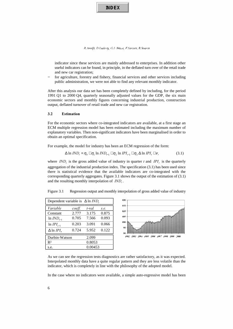
For example, the model for industry has been an ECM regression of the form:

WWWWW,3,,3,,1',1' νηηηη +∆+++=∆ −− ln ln ln ln 312110 (3.1)

where W

,1' is the gross added value of industry in quarter W and W

,3, is the quarterly

aggregation of the industrial production index. The specification (3.1) has been used sincethere is statistical evidence that the available indicators are co-integrated with thecorresponding quarterly aggregates. Figure 3.1 shows the output of the estimation of (3.1)and the resulting monthly interpolation of

W,1' .

Figure 3.1 Regression output and monthly interpolation of gross added value of industry

Dependent variable is W

,1' ln ∆

9DULDEOH FRHII� W�YDO V�H�Constant 2.777 3.175 0.875

1ln −W,1' 0.705 7.566 0.093

1ln −W,3, 0.203 3.091 0.066

W,3,ln ∆ 0.724 5.952 0.122

Durbin-Watson 2.099R² 0.8053s.e. 0.00453

As we can see the regression tests diagnostics are rather satisfactory, as it was expected.Interpolated monthly data have a quite regular pattern and they are less volatile than theindicator, which is completely in line with the philosophy of the adopted model.

In the case where no indicators were available, a simple auto-regressive model has been

��

��

��

��

��

��

��

��


7

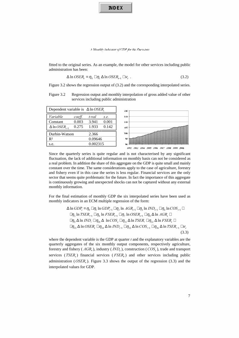
fitted to the original series. As an example, the model for other services including publicadministration has been:

WWW26(526(5 νηη +∆+=∆ −110 ln ln . (3.2)

Figure 3.2 shows the regression output of (3.2) and the corresponding interpolated series.

Figure 3.2 Regression output and monthly interpolation of gross added value of otherservices including public administration


26(5 ln ∆

9DULDEOH FRHII� W�YDO V�H�Constant 0.003 3.941 0.001

1 ln −∆W

26(5 0.275 1.933 0.142


Since the quarterly series is quite regular and is not characterised by any significantfluctuation, the lack of additional information on monthly basis can not be considered asa real problem. In addition the share of this aggregate on the GDP is quite small and mainlyconstant over the time. The same considerations apply to the case of agriculture, forestryand fishery even if in this case the series is less regular. Financial services are the onlysector that seems quite problematic for the future. In fact the importance of this aggregateis continuously growing and unexpected shocks can not be captured without any externalmonthly information.

For the final estimation of monthly GDP the six interpolated series have been used asmonthly indicators in an ECM multiple regression of the form:

+++++=∆ −−−− 141312110 ln ln ln ln ln WWWWW

&26,1'$*5*'3*'3 ηηηηη+∆++++ −−− WWWW

$*526(5)6(576(5 ln ln ln ln 8171615 ηηηη+∆+∆+∆+∆+

WWWW)6(576(5&26,1' ln ln ln ln 1211109 ηηηη

WWWWW76(5&26,1'26(5 νηηηη +∆+∆+∆+∆+ −−− 11611511413 ln ln ln ln

(3.3)

where the dependent variable is the GDP at quarter W and the explanatory variables are thequarterly aggregates of the six monthly output components, respectively agriculture,forestry and fishery (

W$*5 ), industry (

W,1' ), construction (

W&26 ), trade and transport

services (W

76(5 ) financial services (W

)6(5 ) and other services including public

administration (W

26(5 ). Figure 3.3 shows the output of the regression (3.3) and the

interpolated values for GDP.

��

��

��

��

��

��

��

��


8

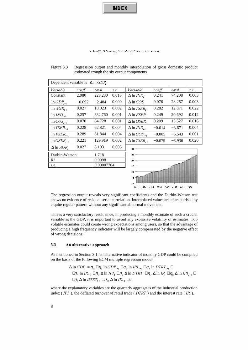
Figure 3.3 Regression output and monthly interpolation of gross domestic productestimated trough the six output components


*'3 ln ∆

9DULDEOH FRHII� W�YDO V�H� 9DULDEOH FRHII� W�YDO V�H�Constant 2.980 228.230 0.013

W,1' ln ∆ 0.241 74.208 0.003

1 ln −W*'3 −0.092 −2.484 0.000W

&26 ln ∆ 0.076 28.267 0.003

1 ln −W$*5 0.027 18.023 0.002W

76(5 ln ∆ 0.282 12.871 0.022

1 ln −W,1' 0.257 332.760 0.001W

)6(5 ln ∆ 0.249 20.692 0.012

1 ln −W&26 0.070 84.728 0.001W

26(5 ln ∆ 0.209 13.527 0.016

1 ln −W76(5 0.228 62.821 0.004 1 ln −∆W

,1' −0.014 −3.671 0.004

1 ln −W)6(5 0.289 81.844 0.004 1 ln −∆W

&26 −0.005 −5.543 0.001

1 ln −W26(5 0.221 129.919 0.002 1 ln −∆W

76(5 −0.079 −3.936 0.020

W$*5 ln ∆ 0.027 8.193 0.003


The regression output reveals very significant coefficients and the Durbin-Watson testshows no evidence of residual serial correlation. Interpolated values are characterised bya quite regular pattern without any significant abnormal movement.

This is a very satisfactory result since, in producing a monthly estimate of such a crucialvariable as the GDP, it is important to avoid any excessive volatility of estimates. Toovolatile estimates could create wrong expectations among users, so that the advantage ofproducing a high frequency indicator will be largely compensated by the negative effectof wrong decisions.

�� $Q�DOWHUQDWLYH�DSSURDFK

As mentioned in Section 3.1, an alternative indicator of monthly GDP could be compiledon the basis of the following ECM multiple regression model:

++++=∆ −−− 1312110 ln ln ln ln WWWW

'757,3,*'3*'3 ηηηη+∆+∆+∆+∆++ −− 1876514 ln ln ln ln ln

WWWWW,3,,5'757,3,,5 ηηηηη

WWW,5'757 νηη +∆+∆+ −− 11019 ln ln

where the explanatory variables are the quarterly aggregates of the industrial productionindex (

W,3, ), the deflated turnover of retail trade (

W'757 ) and the interest rate (

W,5 ).

��

��

��

��

��

��

��

��


9

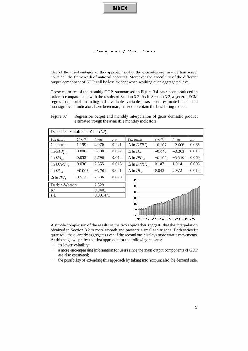
One of the disadvantages of this approach is that the estimates are, in a certain sense,“outside” the framework of national accounts. Moreover the specificity of the differentoutput component of GDP will be less evident when working at an aggregated level.

These estimates of the monthly GDP, summarised in Figure 3.4 have been produced inorder to compare them with the results of Section 3.2. As in Section 3.2, a general ECMregression model including all available variables has been estimated and thennon-significant indicators have been marginalised to obtain the best fitting model.

Figure 3.4 Regression output and monthly interpolation of gross domestic productestimated trough the available monthly indicators


*'3 ln ∆

9DULDEOH &RHII� W�YDO V�H� 9DULDEOH FRHII� W�YDO V�H�Constant 1.199 4.970 0.241

W'757ln ∆ −0.167 −2.608 0.065

1 ln −W*'3 0.888 39.801 0.022W

,5ln ∆ −0.040 −3.203 0.013

1 ln −W,3, 0.053 3.796 0.014 1ln −∆W

,3, −0.199 −3.319 0.060

1ln −W'757 0.030 2.355 0.013 1ln −∆W

'757 0.187 1.914 0.098

1ln −W,5 −0.003 −3.761 0.001 1ln −∆W

,5 0.043 2.972 0.015

W,3,ln ∆ 0.513 7.336 0.070


A simple comparison of the results of the two approaches suggests that the interpolationobtained in Section 3.2 is more smooth and presents a smaller variance. Both series fitquite well the quarterly aggregates even if the second one displays more erratic movements.At this stage we prefer the first approach for the following reasons:− its lower volatility;− a more encompassing information for users since the main output components of GDP

are also estimated;− the possibility of extending this approach by taking into account also the demand side.

��

��

��

��

��

��

��

��


10

�� &RQFOXVLRQV

In this paper the Eurostat strategy for the estimation of a monthly indicator of GDP hasbeen synthetically presented. Results seem to be quite encouraging even if more in-depthanalysis is still needed.

Further work should deal with the following aspects:− monthly extrapolation when a complete quarter is still not available;− dynamic simulation over a given time period to assess the ability of monthly estimates

to produce accurate estimations of quarterly figures;− identification of additional information sources to improve the quality of the estimates

in particular in the services domain;− analysis of the utility of short-term qualitative business and consumer surveys to

extrapolate quantitative variables such as the industrial production index or theconstruction output index, currently used in the estimation process of monthly GDP.

In addition it will be useful to test the impact of seasonal adjustment practices on theinterpolation of quarterly national accounts. For example whether the adoption of a directseasonal adjustment methodology for the Euro-zone quarterly national accounts couldimprove the quality of the monthly estimates, as it is expected from a theoretical point ofview.

Finally it is important to note that, as for all short-term statistics, the usefulness of amonthly GDP is strongly related to the delay of its publication. A detailed analysis has tobe made to investigate the impact of using an incomplete or forecasted set of informationon the quality and the reliability of the GDP estimates. On the basis of such an analysis,Eurostat will decide if a monthly GDP will be calculated and from when onwards such anindicator will be published.

5HIHUHQFHV

[1] Bournay J., Laroque G., (1979), 5pIOH[LRQV�VXU�OD�PpWKRGH�GHODERUDWLRQ�GHV�FRPSWHV�WULPHVWULHOV,Annales de l’INSEE 36, 3-30.

[2] Chow G., Lin A.L., (1971), %HVW�OLQHDU�XQELDVHG�,QWHUSRODWLRQ��'LVWULEXWLRQ�DQG�([WUDSRODWLRQ�RI�7LPH6HULHV�E\�5HODWHG�6HULHV, The Review of Economics and Statistics 53(4), 372-375.

[3] Eurostat, (1999), +DQGERRN�RQ�4XDUWHUO\�1DWLRQDO�$FFRXQWV.[4] Fernández R.B., (1981), $�0HWKRGRORJLF�1RWH�RQ� WKH�(VWLPDWLRQ�RI�7LPH�6HULHV, The Review of

Economics and Statistics 63(3), 471-478.[5] Gregoir S., (1994), 1RWH�RQ�WHPSRUDO�'LVDJJUHJDWLRQ�ZLWK�VLPSOH�G\QDPLF�0RGHOV, Workshop on

Quarterly National Accounts, Paris 5-6 December 1994.[6] Litterman R.B., (1983), $�UDQGRP�:DON��0DUNRY�0RGHO�IRU�WKH�'LVWULEXWLRQ�RI�7LPH�6HULHV, Journal

of Business and Economic Statistics 1(2), 169-173.[7] Pinheiro M., Coimbra C., (1993), 'LVWULEXWLRQ�DQG�([WUDSRODWLRQ�RI�7LPH�6HULHV�E\�5HODWHG�6HULHV

8VLQJ�/RJDULWKPV�DQG�6PRRWKLQJ�3HQDOLWLHV, Economia v.XVII, 359-374.[8] Salazar E.,Smith R., Weale M., Wright S., (1994), ,QGLFDWRUV�RI�PRQWKO\�1DWLRQDO�$FFRXQWV, Workshop

on Quarterly National Accounts, Paris 5-6 December 1994.

Documents

creta Monthly GDP