1

Serious Implications: Forecast Skew Over the Next Decade By Ed Easterling April 6, 2018 Copyright 2018, Crestmont Research (www.CrestmontResearch.com) Forecasts are coveted. We rely upon them every day: weather forecasts, daily commute travel time, people attending an event, etc. In some cases, we plan college savings, home ownership, and retirement based upon forecasts. Generally, we think about specific-point forecasts as mid-ranges. Statisticians call this point the central tendency. It’s the middle or typical value in a probability distribution. Many people envision the peak of a bell-shaped curve. From that lofty perch, the range of outcomes is a set of balanced wings that stretch outward on each side of the forecast. For example, if the high temperature today doesn’t end up being the forecasted 80 degrees, it could just as likely be 79 as it could be 81…or 78 versus 82. Therefore, plan for 80 and expect that the upside range offsets the downside. Yet for some forecasts, the range of outcomes isn’t balanced. For example, as you launch the GPS app for your morning commute, the path shows green with no traffic alerts and the drive time is displayed as 29 minutes. Your GPS calculates travel time based upon speed limits and traffic across the route. Since you don’t speed (right!), you have little ability to beat the estimated time. Yet if traffic is unexpectedly slow or if the stop lights curse your drive that day, your time can slide well past the half hour. You don’t have the same opportunity for a 25-minute cruise as you do for a 35-minute slog. Investment forecasts have much more serious implications than daily commutes—even if it doesn’t seem that way during rush hour! This article will describe and demonstrate the serious implications of forecast skew for long-term stock market returns. Spoiler alert: Most forecasts for stock market returns from Wall Street analysts average near 6% annually. However, there is almost no chance of a 7% annualized return for the next decade, but high chance that it’s between 0% and 6%. This outlook should be empowering, not concerning. There is a lot that can be done by and for investors to achieve success even when returns from the stock market are so far below average. The first step is to recognize the market environment and to understand the principles and drivers of return. Then, the objective is to structure portfolios so they have components that will overperform expectations if the stock market underperforms.

“…there is almost no chance of a 7% annualized return for the next decade, but high chance that it’s between 0% and 6%.”

Crestmont Research

2

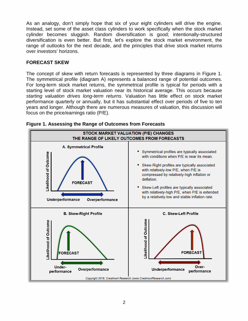
As an analogy, don’t simply hope that six of your eight cylinders will drive the engine. Instead, set some of the asset class cylinders to work specifically when the stock market cylinder becomes sluggish. Random diversification is good; intentionally-structured diversification is even better. But first, let’s explore the stock market environment, the range of outlooks for the next decade, and the principles that drive stock market returns over investors’ horizons. FORECAST SKEW The concept of skew with return forecasts is represented by three diagrams in Figure 1. The symmetrical profile (diagram A) represents a balanced range of potential outcomes. For long-term stock market returns, the symmetrical profile is typical for periods with a starting level of stock market valuation near its historical average. This occurs because starting valuation drives long-term returns. Valuation has little effect on stock market performance quarterly or annually, but it has substantial effect over periods of five to ten years and longer. Although there are numerous measures of valuation, this discussion will focus on the price/earnings ratio (P/E). Figure 1. Assessing the Range of Outcomes from Forecasts

3

The Skew-Right profile (diagram B) reflects the profile early in a secular bull market. Relatively-low market valuation (i.e., low P/E) generally has much more upside than downside. P/E becomes compressed, like a coiled spring, with minimal room to decline and lots of space to expand. This last occurred in the early 1980s and has occurred several times over the past century. The Skew-Left profile (diagram C) reflects conditions when P/E is relatively-high. Just as Icarus found limits to waxed wings, stock market valuation has principles that limit its heights. PRINCIPLES, NOT RANDOMNESS For many readers, the preceding statements about valuation-driven returns will conjure notions of models or theories to explain the supposedly-random nature of the stock market. The logic extends as follows: if the stock market is random from day-to-day and year-to-year, how could it possibly be highly-predictable over longer periods like decades? The misunderstanding of stock market randomness has its roots in three great theories. The first was Harry Markowitz’s Modern Portfolio Theory (MPT), published in 1952. According to MPT, risk drives return and investors are paid only for market risk. Next, in 1970, Eugene Fama published an article that described his Efficient Market Hypothesis (EMH). According to Fama, markets are efficient and stock prices immediately incorporate all available information. As a result, stock picking doesn’t work, so just use MPT to passively buy-and-hold a diversified portfolio of stocks. Last, in 1973, Burton Malkiel published his magnum opus A Random Walk Down Wall Street. Malkiel presented investment advice as he popularized the Random Walk Hypothesis (RWH). Under RWH, stock prices move according to a random walk and therefore cannot be predicted. The Big 3 theories have been combined together and taught to legions of students and Wall Street analysts. The message is clear: Diversify portfolios, don’t try to pick individual stocks, and passively buy-and-hold stocks for successful long-term investing. About half-way through the first generation of indoctrination, the newfound “modern” approach to portfolios was indelibly reinforced with the best-ever secular bull market of the 1980s and ‘90s. But there was just one catch. And Markowitz warned about it in MPT. The leading paragraph of his 1952 paper starts with:

“THE PROCESS OF SELECTING a portfolio may be divided into two stages. The first stage starts with observation and experience and ends with beliefs about the future performances of available securities. The second stage starts with the relevant beliefs about future performances and ends with the choice of portfolio. This paper is concerned with the second stage.”

Markowitz is clear: His model is only as good as your assumptions!

The stock market is random from year-to-year, yet highly predictable over decade-long periods.

4

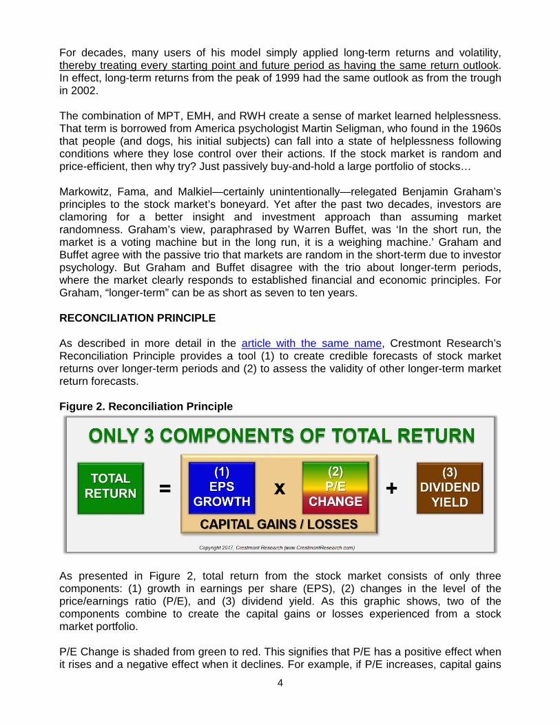
For decades, many users of his model simply applied long-term returns and volatility, thereby treating every starting point and future period as having the same return outlook. In effect, long-term returns from the peak of 1999 had the same outlook as from the trough in 2002. The combination of MPT, EMH, and RWH create a sense of market learned helplessness. That term is borrowed from America psychologist Martin Seligman, who found in the 1960s that people (and dogs, his initial subjects) can fall into a state of helplessness following conditions where they lose control over their actions. If the stock market is random and price-efficient, then why try? Just passively buy-and-hold a large portfolio of stocks… Markowitz, Fama, and Malkiel—certainly unintentionally—relegated Benjamin Graham’s principles to the stock market’s boneyard. Yet after the past two decades, investors are clamoring for a better insight and investment approach than assuming market randomness. Graham’s view, paraphrased by Warren Buffet, was ‘In the short run, the market is a voting machine but in the long run, it is a weighing machine.’ Graham and Buffet agree with the passive trio that markets are random in the short-term due to investor psychology. But Graham and Buffet disagree with the trio about longer-term periods, where the market clearly responds to established financial and economic principles. For Graham, “longer-term” can be as short as seven to ten years. RECONCILIATION PRINCIPLE As described in more detail in the article with the same name, Crestmont Research’s Reconciliation Principle provides a tool (1) to create credible forecasts of stock market returns over longer-term periods and (2) to assess the validity of other longer-term market return forecasts. Figure 2. Reconciliation Principle

As presented in Figure 2, total return from the stock market consists of only three components: (1) growth in earnings per share (EPS), (2) changes in the level of the price/earnings ratio (P/E), and (3) dividend yield. As this graphic shows, two of the components combine to create the capital gains or losses experienced from a stock market portfolio. P/E Change is shaded from green to red. This signifies that P/E has a positive effect when it rises and a negative effect when it declines. For example, if P/E increases, capital gains

5

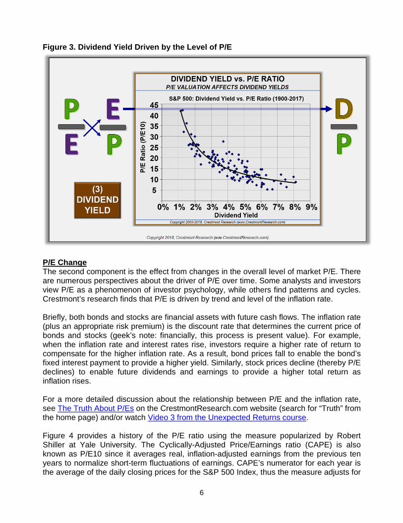
benefit from an increase in the level of valuation regardless of earnings growth. If P/E remains constant, however, then stock prices rise only by the amount of earnings growth. A decline in P/E suppresses capital gains and, at times, can more than offset even strong earnings growth. ASSESSING SKEW Current long-term forecasts for U.S. stock market returns published by many Wall Street firms generally fall in the range of 5% to 6% annually. These forecasts often cover seven to ten years and relate to nominal total return before expenses. Most firms do not detail the contribution of the three components, yet they implicitly assume capital gains of 3% to 4% and dividend yield of 2%. Some firms assume solid earnings growth with modest P/E decline, while others assume plodding earnings growth and no P/E decline. A few firms, the reversion-to-the-meanists, project near 0% returns due their perpetual assumption that P/E is gravitationally-drawn back to its mean. The objective of this section is to detail the plausible range of outcomes for annualized stock market returns over the next decade. If 6% is the forecast, is 8% just as possible as 4%? Is the historical average of 10% within reach with an equal risk on the downside of at least beating cash at 2%? The analysis can be done credibly by aggregating the plausible range for each component. Since the S&P 500 Index is the largest sector by market capitalization, this analysis will be based upon that index. Dividend Yield Let’s first consider dividend yield, which tends to be relatively predictable based upon the level of P/E. As P/E rises, the yield of a given dividend payment declines. Higher prices cause lower dividend yields…and vice versa. This occurs for mathematical reasons. P/E and dividend yield are closely related, as shown in Figure 3. P/E is price (P) divided by earnings (E). The inverse of P/E (i.e., E/P) is known as the earnings yield. Dividend yield is dividend (D) divided by price (i.e., D/P). E/P and D/P have the same denominator in their respective equation—price. Therefore, the relationship of P/E and dividend yield is simply the relationship between earnings and dividends. Since dividends are paid from, and based upon, earnings, the two variables have a direct relationship (and thus the chart in Figure 3 shows a highly-correlated pattern). From today, with dividend yield near 2%, the range of outcomes is largely dependent on any changes in dividend payout policy for S&P 500 companies in the aggregate. Using the historical range of payout rates, the plausible variation for dividend yield is approximately +/- 0.2%. Thus, the highly-likely range for dividend yield from today is 1.8% to 2.2%. Even under scenarios that extend the range, the magnitude of effect on total return is minimal.

6

Figure 3. Dividend Yield Driven by the Level of P/E

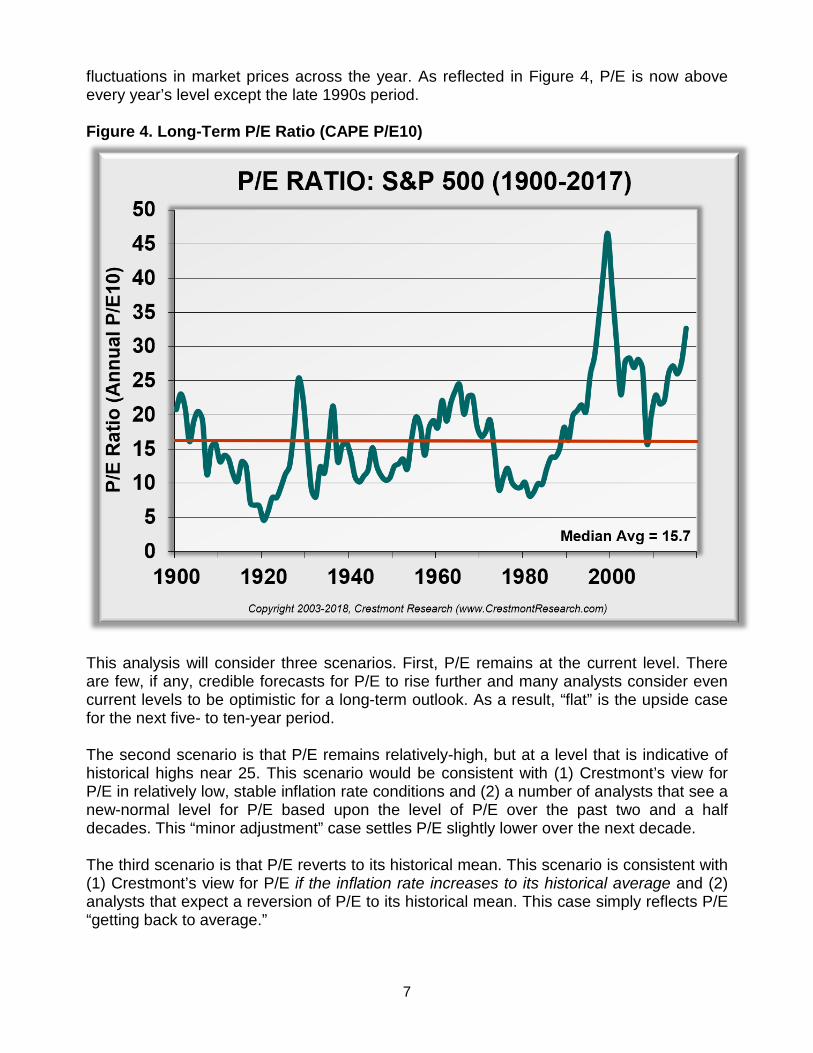
P/E Change The second component is the effect from changes in the overall level of market P/E. There are numerous perspectives about the driver of P/E over time. Some analysts and investors view P/E as a phenomenon of investor psychology, while others find patterns and cycles. Crestmont’s research finds that P/E is driven by trend and level of the inflation rate. Briefly, both bonds and stocks are financial assets with future cash flows. The inflation rate (plus an appropriate risk premium) is the discount rate that determines the current price of bonds and stocks (geek’s note: financially, this process is present value). For example, when the inflation rate and interest rates rise, investors require a higher rate of return to compensate for the higher inflation rate. As a result, bond prices fall to enable the bond’s fixed interest payment to provide a higher yield. Similarly, stock prices decline (thereby P/E declines) to enable future dividends and earnings to provide a higher total return as inflation rises. For a more detailed discussion about the relationship between P/E and the inflation rate, see The Truth About P/Es on the CrestmontResearch.com website (search for “Truth” from the home page) and/or watch Video 3 from the Unexpected Returns course. Figure 4 provides a history of the P/E ratio using the measure popularized by Robert Shiller at Yale University. The Cyclically-Adjusted Price/Earnings ratio (CAPE) is also known as P/E10 since it averages real, inflation-adjusted earnings from the previous ten years to normalize short-term fluctuations of earnings. CAPE’s numerator for each year is the average of the daily closing prices for the S&P 500 Index, thus the measure adjusts for

7

fluctuations in market prices across the year. As reflected in Figure 4, P/E is now above every year’s level except the late 1990s period. Figure 4. Long-Term P/E Ratio (CAPE P/E10)

This analysis will consider three scenarios. First, P/E remains at the current level. There are few, if any, credible forecasts for P/E to rise further and many analysts consider even current levels to be optimistic for a long-term outlook. As a result, “flat” is the upside case for the next five- to ten-year period. The second scenario is that P/E remains relatively-high, but at a level that is indicative of historical highs near 25. This scenario would be consistent with (1) Crestmont’s view for P/E in relatively low, stable inflation rate conditions and (2) a number of analysts that see a new-normal level for P/E based upon the level of P/E over the past two and a half decades. This “minor adjustment” case settles P/E slightly lower over the next decade. The third scenario is that P/E reverts to its historical mean. This scenario is consistent with (1) Crestmont’s view for P/E if the inflation rate increases to its historical average and (2) analysts that expect a reversion of P/E to its historical mean. This case simply reflects P/E “getting back to average.”

8

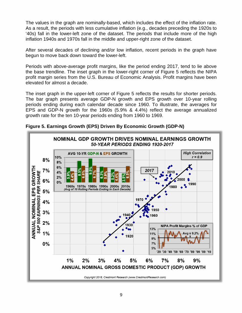
As shown in Figure 4, P/E could go even lower than its historical average. But since technology has yet to develop a means to digitally create a scratch-and-sniff patch with smelling salts, we’ll carefully include that scenario in the summarizing set. Bringing up the rear, we’ll call this case “end of the secular bear.” In summary, if P/E ends the decade at current levels, there is no effect from P/E change on the compounded annual return for the ten-year forecast. If P/E descends to 25, the effect is approximately -2.2% per year. If P/E declines to its long-term average by 2027, the effect on the stock market cuts nearly -6.8% annually from the ten-year forecast. Earnings Growth The third component is earnings growth, which is a bit more complex. The earnings cycle fluctuates dramatically, often with significant increases and decreases from year-to-year. For example, over the past fifty years, reported EPS declined in 30% of the years. Only some of the EPS decline years included recession periods and none of the years had negative nominal growth in GDP for the full year. The business cycle has wider and more frequent swings than the economic cycle. Beyond years with decline, EPS expresses significant magnitude in its variability. Over the past 50 years, 35 of them had gains and declines that were double-digit and exceeded ten percent. Shorter-term surges and falls are poor measures of the contribution of long-term EPS growth to stock market gains. That’s why Benjamin Graham wrote about a seven-year average to normalize EPS and why Robert Shiller uses a ten-year rolling average to normalize EPS for CAPE P/E10. Both Graham and Shiller are seeking to normalize the substantial fluctuations in EPS across business cycles. They use historical reported data to provide a reasonable estimate of the normalized core trend level of earnings to value stocks or the market, respectively. Returning to the fifty-year example, when averaged over ten-year periods, EPS declined during only one of the 41 rolling decades (the ten years ending 2008). The ten-year average EPS drops the standard deviation of annual changes by more than 90% (standard deviation is a statistic for the magnitude of fluctuation). To forecast future earnings growth, we can employ the relationship of earnings to its primary driver, economic growth (as reflected by nominal gross domestic product, GDP-N). Figure 5 includes several complementary graphs that explain the strong relationship between EPS and GDP-N. The main plot diagram reflects EPS growth and GDP growth for each year since 1920. To smooth distortions from the economic and business cycles, each point in the graph reflects the compounded growth rates over fifty-year periods ending 1920 to 2017. The correlation as reflected in the r statistic is 0.9 (1.0 is perfect correlation; 0.9 is considered to be high).

“There are only three sources of return from the stock market: growth in earnings per share (EPS), changes in the level of the price/earnings ratio (P/E), and dividend yield.”

9

The values in the graph are nominally-based, which includes the effect of the inflation rate. As a result, the periods with less cumulative inflation (e.g., decades preceding the 1920s to ‘40s) fall in the lower-left zone of the dataset. The periods that include more of the high inflation 1940s and 1970s fall in the middle and upper-right zone of the dataset. After several decades of declining and/or low inflation, recent periods in the graph have begun to move back down toward the lower-left. Periods with above-average profit margins, like the period ending 2017, tend to lie above the base trendline. The inset graph in the lower-right corner of Figure 5 reflects the NIPA profit margin series from the U.S. Bureau of Economic Analysis. Profit margins have been elevated for almost a decade. The inset graph in the upper-left corner of Figure 5 reflects the results for shorter periods. The bar graph presents average GDP-N growth and EPS growth over 10-year rolling periods ending during each calendar decade since 1960. To illustrate, the averages for EPS and GDP-N growth for the 1960s (5.9% & 4.4%) reflect the average annualized growth rate for the ten 10-year periods ending from 1960 to 1969. Figure 5. Earnings Growth (EPS) Driven By Economic Growth (GDP-N)

10

The most significant point is that EPS growth is slightly slower than GDP-N growth for every period except the 2010s. The 2010s has higher EPS growth because of the substantial increase in profit margins during that period. Over time, EPS growth is expected to be slightly slower than GDP-N growth because economic growth includes the effects of new start-ups and faster-growing small companies. The implication for the next decade is significant. Many economists, including official forecasts from the Congressional Budget Office (CBO) and Federal Open Market Committee (FOMC), expect real GDP growth of approximately 2.0% annually over the next decade. Further, the FOMC’s long-term outlook for the inflation rate is 2.0%. Thus, the official outlook for nominal GDP growth over the next decade is 4.0%. As a result, assuming heightened profit margins are sustained, the reasonable outlook for EPS growth is somewhat less than 4% (3% to 3.5% optimistically). Note that the somewhat slower growth rates of the pre-World War II periods reflect the slightly higher dividend payout rates of that period. This is consistent with research by Merton Miller and Franco Modigliani (and others) that higher dividend payouts are associated with slower growth rates since less capital is retained by companies to support and promote growth. As for determining a reasonable range for EPS growth over the next decade, let’s consider several scenarios. First, a return to historical economic growth rates (before growth became suppressed rates in the early 2000s) would add approximately 1% to real GDP and slightly less to EPS growth. Thus, for the first earnings case, restoring historically-average economic growth (without recession or higher inflation) could drive annualized EPS growth for the next decade to near 4.5%. Next, the current economic expansion will become the second longest on record in May 2018. If history is a guide, one or two recessions are likely during the next decade. For perspective, since 1930 when recessions became less frequent, each calendar decade has had one or two recessions (with two recessions occurring twice as often as one). The historical average for real economic growth includes expansion periods averaging near 4% annually and recessions generally with negative growth. Together, the expansion and recession cycle historically has compounded on average near 3% (before adding the effects of inflation). The first scenario assumed a slow and steady 3% growth without recession. Under this scenario, a recession or two in the next ten years would suppress annualized economic and earnings growth. Although there are variations for this second scenario, a recession would suppress cumulative average EPS growth. This adds an element of caution to the potential return contribution from this component of stock market return. Further adding to the scenarios, any reversion of profit margins from its currently high level will reduce the cumulative growth rate of EPS for the decade. The recent decade’s growth in EPS benefited from margin expansion; a decade with contraction would return those temporary gains.

11

Keep in mind that any forecast for EPS growth that equals or exceeds GDP-N growth implicitly assumes a continued expansion of profit margins from already high levels. Although margins could increase further, that is less likely when periods start with an already lofty level of profits. Some analysts will assert that corporate stock buybacks accelerate earnings growth. That effect is significantly reduced when share issuances and option exercises are included. Further, net share buybacks at current high valuations may have a positive short-term effect on EPS growth, but on average the economic effect to corporate valuation is negative in the longer-term. ADDITIONAL COMMENTS The forecasts in Figure 6 are not comprehensive, yet they are representative. Most of the composite scenarios for stock market returns over the next decade lie somewhere inside the range of -7.3% to +6.7%. This is especially true for scenarios that are internally-consistent. The concept of internal consistency requires that each underlying assumption be applied rationally to all three of the components. For example, the assumption of an increase in the inflation rate could help increase nominal EPS growth. Yet such an increase in the inflation rate would also cause a decline in P/E. The aggregate net effect from an assumption about higher inflation should be considered, not just the effect on one component of total return. One other consideration has not been addressed. It affects every scenario in Figure 6 except Skew-Right “Good.” That scenario assumes historically-average economic growth. The other scenarios assume below-average growth consistent with official FOMC, OMB, and private sector forecasts. For the other scenarios to be internally-consistent, they should include the effect of slower growth on the overall level of P/E. If the overall economy downshifts its growth rate compared to the historical average, the implication is that the fair value for the stock market should downshift accordingly. The effect would be a reduction to the six left-most scenarios in Figure 6. For a more detailed discussion about this effect, see the article Game Changer at CrestmontResearch.com. Yet in the spirit of optimism, let’s allow that internal inconsistency to remain in the analysis with hope that historical economic growth returns in the long-run. IMPLICATIONS Empowerment comes from a confident outlook about the investment environment over investors’ horizons. The range of outcomes for stock market returns over the next decade (2018-2027) reflects annualized returns from -7.3% to +6.7%. The outcome range displays a significant Skew-Left profile. The “upside” from the base case is +1.2%; the “downside” from the base case is -12.8% (i.e., 5.5% minus -7.3%). The skew primarily results from a starting point for P/E that is relatively high. But, the skew is further exacerbated by the current near extreme level of P/E, which is higher than all historical periods other than the late 1990s era. Additionally,

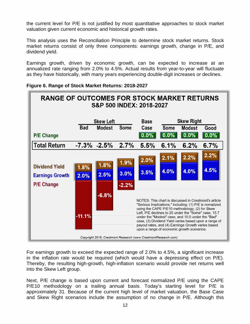
12

the current level for P/E is not justified by most quantitative approaches to stock market valuation given current economic and historical growth rates. This analysis uses the Reconciliation Principle to determine stock market returns. Stock market returns consist of only three components: earnings growth, change in P/E, and dividend yield. Earnings growth, driven by economic growth, can be expected to increase at an annualized rate ranging from 2.0% to 4.5%. Actual results from year-to-year will fluctuate as they have historically, with many years experiencing double-digit increases or declines. Figure 6. Range of Stock Market Returns: 2018-2027

For earnings growth to exceed the expected range of 2.0% to 4.5%, a significant increase in the inflation rate would be required (which would have a depressing effect on P/E). Thereby, the resulting high-growth, high-inflation scenario would provide net returns well into the Skew Left group. Next, P/E change is based upon current and forecast normalized P/E using the CAPE P/E10 methodology on a trailing annual basis. Today’s starting level for P/E is approximately 31. Because of the current high level of market valuation, the Base Case and Skew Right scenarios include the assumption of no change in P/E. Although this

13

assumption is optimistic, it is consistent with many of the forecasts provided by industry analysts. Readers should take this into consideration when reviewing the range of outcomes and/or when developing their own forecasts. The Skew Left scenarios include the assumption that P/E declines to 25 under the “Some” case, 15.7 under the “Modest” case, and 10.0 under the “Bad” case. The percentage effect reflected in the red portion of the bar graphs in Figure 6 is the approximate effect of P/E declining to those assumed levels over a ten-year period. Last, dividend yield is based upon a range of dividend payouts using historical ranges. The most significant factor driving dividend yield is the starting level of P/E for the ten-year period. With P/E relatively high, dividend yield is destined to be relatively low. Investment Strategy This discussion focused on assessing the market environment over investors’ horizons. The goal was to provide useful insights and personal confidence about the next decade and longer. There are many other sources dedicated to providing specific investment solutions or shorter-term market perspectives; hopefully this discussion will be helpful toward structuring your portfolio or selecting the right professional for assistance. Across the scenarios in Figure 6, it’s clear that risk management is particularly important during high P/E periods. The skill of portfolio management and investment selection can add tremendous value for investors. Since the valuation level at the start of the period drives future returns, today’s relatively high valuation level means that we should expect below-average returns for the next decade and longer. This does not mean that all years will be below-average—quite to the contrary. The stock market presents significant variability across individual years. The recognition of below-average returns for the foreseeable future can be empowering. Beyond its importance for planning, the outlook for stock market returns—and, especially, the plausible range for the outlook—provides important insights for investing. First, compared to historical averages, stocks are much less competitive with other asset classes in the current environment. Stocks remain an important asset class for portfolios, but with a heightened responsibility to seek good value and manage for risk. Further, it is incumbent upon investors and financial advisors to accurately assess the relative return and risk potential of alternatives to equities in a portfolio. Although such extra efforts added relatively little return during the secular bull market of the 1980s and ‘90s, the incremental value to portfolios over the next decade can be significant. As for the appropriate investment strategy: emphasize the more active and diversified “rowing” strategies over the more passive “sailing” strategies within investment portfolios. Ed Easterling is the author of Probable Outcomes: Secular Stock Market Insights and the award-winning Unexpected Returns: Understanding Secular Stock Market Cycles. He is currently the founder and president of Crestmont Research and previously served as an adjunct professor and taught the course on alternative investments and hedge funds for MBA students at SMU in Dallas, Texas. Mr. Easterling publishes provocative research and graphical analyses on the financial markets at CrestmontResearch.com.