_____________________________________________________________________

CREDIT Research Paper

No. 11/08

_____________________________________________________________________

AGGREGATION VERSUS HETEROGENEITY

IN CROSS-COUNTRY GROWTH EMPIRICS

by

Markus Eberhardt and Francis Teal

Abstract

The cross-country growth literature commonly uses aggregate economy datasets such

as the Penn World Table (PWT) to estimate homogeneous production function or

convergence regression models. Against the background of a dual economy

framework this paper investigates the potential bias arising when aggregate economy

data instead of sectoral data is adopted in macro production function regressions.

Using a unique World Bank dataset we estimate production functions in agriculture

and manufacturing for a panel of 41 developing and developed countries (1963-

1992). We employ novel empirical methods which can accommodate technology

heterogeneity, variable nonstationarity and the breakdown of the standard cross-

section independence assumption. We focus on technology heterogeneity across

sectors and countries and the potential for biased estimates due to aggregation and

empirical misspecification, relying on both theory and empirical evidence. Using data

for a stylised aggregate economy made up of agricultural and manufacturing sectors

we confirm substantial bias in the technology coefficients and thus any total factor

productivity measures computed. Our empirical findings imply that sectoral structure

is of crucial importance in the analysis of growth and development, thus

strengthening the recent revival of research on structural change in development

economics.

JEL Classification: dual economy model; cross-country production function;

aggregation bias; technology heterogeneity; common factor model; panel time series

econometrics

Keywords: O47, O11, C23

_____________________________________________________________________

Centre for Research in Economic Development and International Trade,

University of Nottingham

_____________________________________________________________________

CREDIT Research Paper

No. 11/08

_____________________________________________________________________

AGGREGATION VERSUS HETEROGENEITY

IN CROSS-COUNTRY GROWTH EMPIRICS

by

Markus Eberhardt and Francis Teal

Outline

1 Introduction

2 Technology heterogeneity

3 An Empirical Model of A Dual Economy

4 Empirical Results

5 Aggregation bias

6 Concluding Remarks

References

Appendix and Technical Appendix

The Authors

Markus Eberhardt is a lecturer in the School of Economics, University of

Nottingham, and a research associate at the Centre for the Study of African

Economies (CSAE), Department of Economics, University of Oxford. Francis Teal is

a reader in the Department of Economics, University of Oxford and Deputy Director

of CSAE. Corresponding Author: markus.eberhardt@nottingham.ac.uk

Acknowledgements

We are grateful to Harald Badinger, Anindya Banerjee, Alberto Behar, Steve Bond,

Josep Carrion-i-Silvestre, Areendam Chanda, Gerdie Everaert, Hashem Pesaran,

Hildegunn Stokke, Charalambos Tsangarides and Dietz Vollrath for useful comments

and suggestions. We further benefited from comments during seminar presentations at

Oxford, Manchester and Birmingham as well as the CSAE Annual Conference,

Oxford; the 13th Applied Economics Meeting, Seville; the 16th International Panel

Data Conference, Amsterdam; and the 7th Annual Meeting of the Irish Society of

New Economists, Dublin. All remaining errors are our own. The first author is

grateful for financial support from the UK Economic and Social Research Council

[grant numbers PTA-031-2004-00345 and PTA-026-27-2048]; and the Bill and

Melinda Gates Foundation.

_____________________________________________________________________

Research Papers at www.nottingham.ac.uk/economics/credit/

1 Introduction

In the early literature on developing countries a distinction was made between the processes of economic

development and of economic growth. Economic development was seen to be a process of structural

transformation by which in Arthur Lewis’ frequently cited phrase an economy which was “previously saving

and investing 4 or 5 percent of its national income or less, converts itself into an economy where voluntary

savings is running at about 12 to 15 percent of national income” (Lewis, 1954, p.155). An acceleration

in the investment rate was only one part of this process of structural transformation; of equal importance

was the process by which an economy moved from a dependence on subsistence agriculture to one where

an industrial modern sector absorbed an increasing proportion of the labour force (e.g. Jorgensen, 1961;

Ranis & Fei, 1961; Robinson, 1971). In contrast to these models of “development for backward economies”

(Jorgensen, 1961, p.309), where duality between the modern and traditional sectors was a key feature of

the model, was the analysis of economic growth in developed economies.1 Here the processes of factor

accumulation and technical progress occur in an economy which is already ‘developed’, in the sense that it

has a modern industrial sector and agriculture has ceased to be a major part of the economy (e.g. Solow,

1956; Swan, 1956).

The literature begun in the early 1990s has yielded a large array of models in which there has been in-

creasing interaction between the theory and the empirics (Durlauf & Quah, 1999; Easterly, 2002; Durlauf,

Johnson, & Temple, 2005). The latter continue to be dominated by an empirical version of the aggregate

Solow-Swan model (Temple, 2005) with much of the empirical debate focusing on the roles of factor ac-

cumulation versus technical progress (Young, 1995; Klenow & Rodriguez-Clare, 1997a, 1997b; Easterly &

Levine, 2001; Baier, Dwyer, & Tamura, 2006). While there is some new theoretical and empirical work

using a dual economy model (e.g. Vollrath, 2009a, 2009b; Lin, 2011; McMillan & Rodrik, 2011; Page,

2011), this is largely absent from textbooks on economic growth and has not been the central focus of

attention for most of the empirical analyses (Temple, 2005). A primary reason for the focus has been the

availability of data. The Penn World Table (PWT) dataset (most recently, Heston, Summers, & Aten, 2011)

and the Barro-Lee data on human capital (most recently, Barro & Lee, 2010) have supplied macro-data

which ensure that the aggregate human capital-augmented Solow-Swan model can be readily estimated.

However, somewhat underappreciated by the applied empirical literature, a team at the World Bank has

developed comparable sectoral data for agriculture and manufacturing (Crego, Larson, Butzer, & Mundlak,

1998) that enables a closer matching between a dual economy framework and the data, which we seek to

exploit in this paper.

Cross-country growth regressions represent one of the most active fields of empirical analysis within ap-

plied development economics, however the viability of this empirical approach has been seriously ques-

tioned over the past decade and at present these methods are deeply unfashionable. We have argued

elsewhere that much can be learned from cross-country empirics provided the empirical setup allows for

greater flexibility in the estimation equation and recognises the salient data properties of macro panel

datasets (Eberhardt & Teal, 2011). Methods developed in the emerging panel time series literature

(Coakley, Fuertes, & Smith, 2006; Pesaran, 2006; Bai, 2009) can go further in providing robust estimation

and inference for nonstationary panel data where variable series may be correlated across countries and

1We refer to ‘dual economy models’ as representing economies with two stylised sectors of production (agriculture andmanufacturing). ‘Technology’ and ‘technology parameters’ refer to the coefficients on capital and labour in the productionfunction model (elasticities with respect to capital and labour), not Total Factor Productivity (TFP) or its growth rate (tech-nical/technological progress).

1

where global shocks such as the recent financial crisis are likely to impact all countries in the sample,

albeit to a different extent.

This paper, providing empirical analysis of panel data for developing and developed economies, sets out to

address two main objectives: (i) rather than using a calibrated dual economy model for quantitative anal-

ysis we provide empirical estimates for technology coefficients in sectoral production functions. Our main

concern here is the assumption of common technology parameters across countries, which is questionable

from an economic theory standpoint and can be investigated in the data. (ii) We estimate a ‘stylised’ aggre-

gate production function model from agriculture and manufacturing data, and compare results with those

from disaggregated regressions. This will allow us to judge whether neglecting a dual economy structure

leads to bias in the empirical technology coefficients. We use ‘true’ aggregate data from PWT to indicate

whether this behaves in a similar fashion to our aggregated data.

Our findings indicate that allowing sectors and countries to have different technology from each other

is important to obtain unbiased parameter estimates and by implication reliable TFP estimates. Our ag-

gregation analysis shows that there is a systematic bias in the capital coefficient when aggregate rather

than sector-level data are used. It is thus crucial to take account of the sectoral structure of an economy

even when the research question investigated does not explicitly relate to this. Our empirical analysis was

enabled by the unique World Bank dataset on agriculture and manufacturing, it is however important to

stress from the outset that we do not call for a replacement of aggregate economy studies with parallel

sectoral investigation. For alternative research questions the use of data from one or the other sector in ad-

dition to aggregate economy data may be sufficient. There are at least two existing data sources, namely

the FAO for data on agriculture and UNIDO for data on manufacturing, which are ideally suited to carry

out this type of analysis that can account for sectoral structure, for a large number of countries and over a

substantial time period. A recent example in this vein is the work on aid, Dutch Disease and manufacturing

exports by Rajan and Subramanian (2010).

The remainder of the paper is organised as follows: Section 2 motivates technology heterogeneity across

sectors and countries. In Section 3 we introduce an empirical specification of our dual economy frame-

work, discuss the data and briefly review the empirical methods and estimators employed. Section 4

reports and discusses empirical findings at the sector-level. Section 5 then reviews the existing litera-

ture on potential bias in aggregate economy data and presents empirical findings from stylised and PWT

aggregate data. Section 6 summarizes and concludes.

2 Technology heterogeneity

2.1 Technology Heterogeneity across Sectors

From a technical point of view, an aggregate production function only offers an appropriate construct in

cross-country analysis if the economies investigated do not display large differences in sectoral structure

(Temple, 2005), since a single production function framework assumes common production technology

across all ‘firms’ facing the same factor prices. Take two distinct sectors within this economy, assuming

marginal labour product equalisation and capital homogeneity across sectors, and Cobb-Douglas-type pro-

duction technology. Then if technology parameters differ between sectors, aggregated production technol-

ogy cannot be of the (standard) Cobb-Douglas form (Stoker, 1993; Temple & Wößmann, 2006). Finding

2

differential technology parameters in sectoral production function estimation thus is potentially a serious

challenge to treating production in form of an aggregated function.

An alternative motivation for a focus on sector-level rather than aggregate growth across countries runs

as follows: it is common practice to exclude oil-producing countries from any aggregate growth analy-

sis, since “the bulk of recorded GDP for these countries represents the extraction of existing resources,

not value added” (Mankiw, Romer, & Weil, 1992, p.413). The underlying argument is that sectoral ‘dis-

tortions’, such as resource wealth, justify the exclusion of the country observations. By extension of the

same argument, we could suggest that given the large share of agriculture in GDP for countries such as

Malawi (25-50%), India (25-46%) or Malaysia (8-30%) over the period 1970-2000, these countries should

be excluded from any aggregate growth analysis since a significant share of their aggregate GDP derives

from a single resource, namely land.2 Sector-level analysis, in contrast, does not face these difficulties,

since sectors such as manufacturing or agriculture are defined closely enough to represent a reasonably

homogeneous conceptual construct.

2.2 Technology Heterogeneity across Countries

A theoretical justification for heterogeneous technology parameters across countries can be found in the

‘new growth’ literature. This strand of the theoretical growth literature argues that production functions

differ across countries and seeks to determine the sources of this heterogeneity (Durlauf, Kourtellos, &

Minkin, 2001). As Brock and Durlauf (2001, p.8/9) put it: “. . . the assumption of parameter homogeneity

seems particularly inappropriate when one is studying complex heterogeneous objects such as countries”.

The model by Azariadis and Drazen (1990) can be seen as the ‘grandfather’ for many of the theoretical

attempts to allow for countries to possess different technologies from each other (and/or at different

points in time). Further theoretical papers lead to multiple equilibria interpretable as factor parameter

heterogeneity in the production function (e.g. Murphy, Shleifer, & Vishny, 1989; Durlauf, 1993; Banerjee

& Newman, 1993). Further challenge to the assumption of common technology is provided by the ‘appro-

priate technology’ literature, which argues that different technologies are appropriate to different factor

endowments (e.g. Basu & Weil, 1998). Under this explanation, global R&D leaders develop productivity-

enhancing technologies that are suitable for their own capital-labour ratios and cannot be used effectively

by poorer countries and so the latter do not develop. Empirical evidence which lends some support to this

hypothesis can be found, among others, in Clark (2007) and Jerzmanowski (2007). A simpler justification

for heterogeneous production functions is offered by Durlauf et al. (2001, p.929): the Solow model was

never intended to be valid in a homogeneous specification for all countries, but may still be a good way

to investigate each country, i.e. if we allow for parameter differences across countries. Recent empiri-

cal evidence employing specifications that support technology heterogeneity includes Pedroni (2007) and

Cavalcanti, Mohaddes, and Raissi (forthcoming).

2The quoted shares are from the World Development Indicators database (World Bank, 2008). For comparison, maximumshare of oil revenue in GDP, computed as the difference between ‘industry share in GDP’ and ‘manufacturing share in GDP’ fromthe same database yields the following ranges for some of the countries omitted in Mankiw et al. (1992): Iran (12-51%), Kuwait(15-81%), Gabon (28-60%), Saudi Arabia (29-67%).

3

3 An Empirical Model of A Dual Economy

In seeking to understand processes of growth at the macro-level, empirical work has focused primarily

on an aggregate production specification (Temple, 1999). While duality has featured prominently in

theoretical developments there has been only a very limited matching of this theory to empirical models.

This disjunction between theory and testing has reflected in large part the availability of data. In this

paper we employ a large-scale cross-country dataset made publicly available by the World Bank in 2003

(Crego et al., 1998) which allows us to specify manufacturing and agricultural production functions and

thus provides a macro-model of a dual economy that can be compared with the single sector models

dominating the empirical literature. In the following we first present a general empirical specification

for our sector-specific analysis of agriculture and manufacturing. Next we review a number of empirical

estimators, focusing on those arising from the recent panel time series literature, before we briefly discuss

the data.

3.1 Empirical Specification

Our empirical framework adopts a ‘common factor’ representation for a standard log-linearised Cobb-

Douglas production function model. Each sector/level of aggregation (agriculture, manufacturing, aggre-

gate(d) data) is modelled separately — for ease of notation we do not identify this multiplicity in our

general model. Let

yi t = β′i xi t + ui t ui t = αi +λ′i ft + εi t (1)

xmit = πmi + δ′mi gmt +ρ1mi f1mt + . . .+ρnmi fnmt + vmit (2)

ft = %′ft−1+ωt and gt = κ

′gt−1+ εt (3)

for i = 1, . . . , N countries, t = 1, . . . , T time periods and m = 1, . . . , k inputs.3 Equation (1) represents

the production function model, with y as sectoral or aggregated value-added and x as a set of inputs:

labour, physical capital stock, and a measure for natural capital stock (arable and permanent crop land)

in the agriculture specification (all variables are in logs). We consider additional inputs (human capital,

livestock, fertilizer) as robustness checks for our general findings (results available on request). The output

elasticities associated with each input (βi) are allowed to differ across countries.

For unobserved TFP we employ the combination of a country-specific TFP level (αi) and a set of common

factors (ft) with country-specific factor loadings λi — TFP is thus in the spirit of a ‘measure of our

ignorance’ (Abramowitz, 1956), driven by some ‘latent’ processes that are either difficult to measure or

truly unobservable. Equation (3) provides some structure for these unobserved common processes, which

are modelled as simple AR(1) processes, where we do not exclude the possibility of unit root processes

(% = 1, κ = 1) leading to nonstationary observables and unobservables. Note that from this the potential

for spurious regression results arises if the empirical equation is misspecified.

Equation (2) details the evolution of the set of inputs; crucially, some of the same processes determining

the evolution of inputs are also assumed to be driving TFP in the production function equation. Eco-

nomically, this implies that the processes that make up TFP (e.g. knowledge, innovation or absorptive

capacity) are affecting choices over inputs, i.e. the accumulation of capital stock, the evolution of the

3Further, f ·mt ⊂ ft and the error terms εi t , vmit , ωt and εt are white noise.

4

labour force and (in the agriculture equation) the area of land under cultivation, while at the same time

affecting the production of output directly. Simply put, technical progress (often taken as a synonym for

TFP) affects both production and the choice of productive inputs. Econometrically, this setup leads to

endogeneity whereby the regressors are correlated with the unobservables, making it difficult to identify

βi separately from λi and ρi (Kapetanios, Pesaran, & Yamagata, 2011).4 A conceptual justification for the

pervasive character of unobserved common factors is provided by the nature of macro-economic variables

in a globalised world, where economies are strongly connected to each other and latent forces drive all of

the outcomes. The presence of such latent factors makes it difficult to argue for the validity of traditional

approaches to causal interpretation of cross-country empirical analyses. Instrumental variable estimation

in cross-section growth regressions or Arellano and Bond (1991)-type lag-instrumentation in pooled panel

models are both invalid in the face of common factors and/or heterogeneous equilibrium relationships

(Pesaran & Smith, 1995; Lee, Pesaran, & Smith, 1997). Although we consider these types of estimators in

our study, our focus is on the recent panel time series estimators which address nonstationarity, parame-

ter heterogeneity and cross-section dependence. The following section introduces these methods in some

more detail.

3.2 Empirical Implementation

Our empirical setup incorporates a large degree of flexibility with regard to the impact of observable and

unobservable inputs on output. Empirical implementation will necessarily lead to different degrees of

restrictions on this flexibility, which will then be formally tested: the emphasis is on comparison of dif-

ferent empirical estimators allowing for or restricting the heterogeneity in observables and unobservables

outlined above. The following 2× 2 matrix indicates the assumptions implicit in the various estimators

implemented below.5 We confine results for the estimators marked with stars to the Technical Appendix

to save space.

Impact of Unobservables:

COMMON IDIOSYNCRATIC

Production Technology: COMMON POLS, 2FE, CCEP,

GMM?, PMG? CPMG?

IDIOSYNCRATIC MG, FDMG CMG

The panel time series econometric approach is given particular attention in this study for a number of

reasons (for a detailed discussion see Eberhardt & Teal, 2011). Firstly, we know that many macro vari-

ables are potentially nonstationary (e.g. Nelson & Plosser, 1982; Granger, 1997; Pedroni, 2007), which

is confirmed for the variables in our data in the Technical Appendix. When variables are nonstationary,

standard regression output has to be treated with extreme caution, since results are potentially spurious.

Provided variables are cointegrated we can nevertheless establish long-run equilibrium relationships in the

4This is the same concern that micro econometricians refer to as ‘transmission bias’ in the analysis of firm-level productivity.See Eberhardt and Helmers (2010) for a detailed review of the micro literature.

5Abbreviations: POLS — Pooled OLS, 2FE — 2-way Fixed Effects, GMM — Arellano and Bond (1991) Difference GMM andBlundell and Bond (1998) System GMM, MG — Pesaran and Smith (1995) Mean Group (with linear country trends), FDMG —dto. with variables in first difference and country drifts, PMG — Pesaran, Shin, and Smith (1999) Pooled Mean Group estimator,CPMG — dto. augmented with cross-section averages following Binder and Offermanns (2007), CCEP/CMG — Pesaran (2006)Common Correlated Effects estimators. Note that our POLS model is augmented with T − 1 year dummies.

5

data. The practical indication of cointegration is when regressions yield stationary residuals, whereas non-

stationary residuals indicate a potentially spurious regression. Panel time series estimators can address the

concern over spurious regression and we investigate the residuals of each empirical model using panel unit

root tests. Secondly, panel time series methods allow for parameter heterogeneity across countries, which

as motivated above is of great interest in our analysis. Thirdly, panel time series methods can address the

problems arising from cross-section correlation. Whether this is the result of common economic shocks or

local spillover effects, cross-section correlation can potentially induce serious bias in the estimates, since

the impact assigned to an observed covariate in reality confounds its impact with that of the unobservable

processes. A recent empirical illustration for this is provided in Eberhardt, Helmers, and Strauss (forth-

coming), showing that conventional approaches to measuring the impact of R&D on industry productivity

actually yield the combined effect of R&D and ‘knowledge spillovers’ between industries. Although the

panel time series approach does not allow us to quantify their impact, common shocks and local spillovers

can be accommodated in the empirical analysis to obtain unbiased technology coefficients for the observ-

able inputs. We will employ diagnostic tests to analyse each model’s residuals for the presence/absence of

cross-section dependence.

In the following we introduce the Common Correlated Effects (CCE) estimators developed in Pesaran

(2006) and extended to nonstationary variables in Kapetanios et al. (2011) since there are at present rela-

tively few applied studies which employ them (examples include Cavalcanti et al., forthcoming; Eberhardt

et al., forthcoming; Holly, Pesaran, & Yamagata, 2010; Moscone & Tosetti, 2010).6 The CCE estimators

augment the regression equation with cross-section averages of the dependent ( yt) and independent vari-

ables (xt) to account for the presence of unobserved common factors with heterogeneous impact. For the

Mean Group version (CMG), the individual country regression is specified as

yi t = ai + b′ixi t + c0i yt +

k∑

m=1

cmi xmt + ei t (4)

whereupon the parameter estimates bi are averaged across countries akin to the Pesaran and Smith (1995)

Mean Group estimator. The pooled version (CCEP) is specified as

yi t = ai + b′xi t +

N∑

j=1

c0i( yt D j) +k∑

m=1

N∑

j=1

cmi( xmt D j) + ei t (5)

where the D j represent country dummies.7

In order to get an insight into the workings of this approach, consider the cross-section average of our

model in equation (1): as the cross-section dimension N increases, given εt = 0, we get

yt = α+ β′xt + λ

′ft ⇔ ft = λ−1( yt − α− β′xt) (6)

This simple derivation indicates a powerful insight: working with cross-sectional means of y and x can

account for the impact of unobserved common factors (TFP) in the production process. Given the assumed

6We abstract from discussing the standard panel estimators here in great detail and refer to the overview articles by Coakleyet al. (2006), Bond and Eberhardt (2009) and Bond (2002) for more information. We also investigate the Pooled Mean Group(PMG) estimator by Pesaran et al. (1999). We further implement a simple extension to the PMG where we include cross-sectionaverages of the dependent and independent variables (CPMG), as suggested in Binder and Offermanns (2007).

7Thus in the MG version we have N individual country regressions with 2k + 2 RHS variables and in the pooled version asingle regression equation with k+ (k+ 2)N RHS variables.

6

heterogeneity in the impact of unobserved factors across countries (λi) the estimator is implemented in

the fashion detailed above, which allows for each country i to have different parameter estimates on yt

and the xt . Simulation studies (Pesaran, 2006; Coakley et al., 2006; Kapetanios et al., 2011; Pesaran

& Tosetti, 2011) have shown that this approach performs well even when the cross-section dimension

N is small, when variables are nonstationary, cointegrated or not, subject to structural breaks and/or in

the presence of local spillovers and global/local business cycles. In the present study we implement two

versions of the CCE estimators in the sector-level regressions: a standard form as described above; and a

variant which includes the cross-section averages of the input and output variables in the own as well as

the other sector. The latter specification allows for cross-section dependence across sectors, albeit at the

cost of a reduction in degrees of freedom. It is conceivable that the evolution of the agricultural sector

of developing countries influences that of the wider economy in general and the manufacturing sector in

particular, such that this extension is sensible in the dual economy context.

This completes our discussion of the empirical implementation within each sector/level of aggregation.

It is important to emphasise that our empirical results do not represent some form of (econometric)

methodology-based data mining: we have clearly set out that each of the estimators employed implies

specific assumptions about the empirical equation, which translate one-to-one into economic theory. Het-

erogeneity in the impact of observables and unobservables across countries can be directly interpreted as

differences in the production technology and common/differential TFP evolution across countries. The

above discussion suggests that from an economic theory standpoint there are reasons to prefer a more

flexible approach, however we do not impose this on the data. Instead we use established econometric

diagnostics (tests for residual stationarity and cross-section independence) to identify the models that are

rejected and those that are supported by the data.

3.3 Data

Descriptive statistics and a more detailed discussion of the data can be found in the Appendix. We conduct

all empirical analysis with four datasets:

(1) for the agricultural sector, building on the sectoral investment series developed by Crego et al. (1998)

and output from the World Development Indicators (WDI; World Bank, 2008), as well as sectoral

labour and land data from FAO (2007);

(2) for the manufacturing sector, building on the sectoral investment series developed by Crego et al.

(1998), output data from the WDI and labour data from UNIDO (2004);

(3) for a stylised aggregate economy made up of the aggregated data for the agriculture and manufac-

turing sectors;8

(4) for the aggregate economy, building on data provided by the Penn World Table (PWT; we use version

6.2, Heston, Summers, & Aten, 2006).

The capital stocks in the agriculture, manufacturing and PWT samples are constructed from investment

series following the perpetual inventory method (see Klenow & Rodriguez-Clare, 1997b, for details), for

the aggregated sample we simple added up the sectoral capital stocks. Comparison across sectors and

with the stylised aggregate sector is possible due to the efforts by Crego et al. (1998) in providing sec-

toral investment data for agriculture and manufacturing. All monetary values in the sectoral and stylised

aggregated datasets are transformed into US$ 1990 values (in the capital stock case this transformation

8We sum the values for value-added, capital stock (both in per worker terms) and labour and then take the logarithms.

7

is applied to the investment data), following the suggestions in Martin and Mitra (2002). Given concerns

that the stylised aggregate economy data may not represent a sound representation of true aggregate

economy data we have adopted the PWT data, which measures monetary values in International $ PPP,

as a benchmark for comparison — despite a number of vocal critics (e.g. Johnson, Larson, Papageor-

giou, & Subramanian, 2009) the latter is without doubt the most popular macro dataset for cross-country

empirical analysis.9

Our sample is an unbalanced panel10 for 1963 to 1992 made up of 41 developing and developed countries

with a total of 928 observations (average T = 22.6) — our desired aim to compare estimates across

the four datasets requires us to match the same sample, thus reducing the number of observations to

the smallest common denominator. Only eight countries in our sample are in Africa, while around half

are present-day ‘industrialised economies’ — these numbers are however deceiving if one recalls that

structural change and development in many of the latter has been primarily achieved during our period

of study. For instance, it bears reminding that prior to 1964, GDP per capita was higher in Ghana than

in South Korea. In 1970 the share of agricultural value-added in GDP for Finland, Ireland, Portugal and

South Korea amounted to 13%, 16%, 31% and 26% respectively, while the 1992 figures are 5%, 8%,

7% and 8% — strong evidence of economies undergoing structural change. A detailed description of our

sample is available in Table A-I, descriptive statistics are provided in Table A-II for each sample.

4 Empirical Results

Panel unit root and cross-section dependence tests have been confined to the Technical Appendix of the

paper. We adopt the Pesaran (2007) CIPS panel unit root test to analyse the time series properties of each

variable series. Results (see Table TA-1) strongly suggest that variables in levels for the agriculture and

manufacturing data as well as the two aggregate economy representations are nonstationary.

A number of formal and informal procedures to investigate cross-section correlation in the data were

carried out. Results (see Table TA-2) indicate high average absolute correlation coefficients for the data

in log levels and even in the data represented as growth rates. Formal tests for cross-section dependence

(Pesaran, 2004; Moscone & Tosetti, 2009) reject cross-section independence in virtually all variable series

tested.

In the following we discuss the empirical results from sectoral production function regressions for agri-

culture and manufacturing respectively, first assuming technology parameter homogeneity (Section 4.1)

and then allowing for differential technology across countries (Section 4.2). For all regression models we

report residual diagnostic tests including the Pesaran (2007) panel unit root test (we summarise results

using I(0) for stationary, I(1) for nonstationary residuals, with I(1)/I(0) indicating ambiguous results) and

the Pesaran (2004) CD test (H0: cross-section independence), which we take to build our judgement for a

preferred empirical model.

9We are of course aware that the difference in deflation between our sectoral and stylised aggregated data on the one hand andPWT on the other makes them conceptually very different measures of growth and development: the former emphasise tradablegoods production whereas the latter puts equal emphasis on tradable and non-tradable goods and services. However, we believethat these differences are comparatively unimportant for estimation and inference in comparison to the distortions introduced byneglecting the sectoral makeup and technology heterogeneity of economies at different stages of economic development.

10We do not account for missing observations in any way. The preferred empirical specifications presented below are based onheterogeneous parameter models, where arguably the unbalancedness (25% of observations in the balanced panel are missing)comes less to bear than in the homogeneous models due to the averaging of estimates.

8

Note that the empirical model implemented expresses all variables in per worker terms (in logs). The

inclusion of the log labour variable then indicates/tests the deviation from constant returns to scale (i.e.

βL+βK (+βN )−1): a positive (negative) significant coefficient on log labour points to increasing (decreas-

ing) returns, an insignificant one to constant returns. The coefficient on labour in the regression is not

the output elasticitiy with respect to labour, which we also report in a lower panel of each table (‘Implied

βL ’), along with the returns to scale (‘Implied RS’). This setup allows for an easy imposition of constant

returns by dropping the log labour variable from the model. In each table Panel (A) shows results with no

restrictions on returns to scale, whereas Panel (B) imposes CRS.

4.1 Pooled Models

Table 1 presents the empirical results for agriculture and manufacturing. Beginning with agriculture, the

empirical estimates for the models [1] and [2] neglecting cross-section dependence are quite similar,

with the capital coefficient around .63 and statistically significant decreasing returns to scale. The land

coefficient is insignificant except in the 2FE model, where it carries a negative sign. Diagnostic tests

indicate that the residuals in these models are cross-sectionally dependent, and that the levels models

(POLS, 2FE) have nonstationary residuals and thus may represent spurious regressions. In the presence

of nonstationary residuals the t-statistics in the levels models are invalid (Kao, 1999) and have commonly

been found to vastly overstate the precision of the estimates (Bond & Eberhardt, 2009). The two CCEP

models yield stationary and cross-sectionally independent residuals, capital coefficients of around .5 and

insignificant land coefficients. Imposition of CRS (Panel (B)) does not change these results substantially,

with the exception of the 2FE estimates, where the land variable (previously negative and significant) is

now insignificant and the capital coefficient has become further inflated. Land is still insignificant, but at

least in model [3] has a plausible coefficient estimate.

In the manufacturing data the models [5] and [6] ignoring cross-section dependence yield increasing

returns to scale and capital coefficients in excess of .85. Residuals again display nonstationarity but the

CD tests now imply that they are cross-sectionally independent. Surprisingly the standard CCEP model in

[7], with a capital coefficient of around .5 (like in agriculture) does not pass the cross-section correlation

test. However, further accounting for cross-sector dependence in [8] yields favourable diagnostics and a

similar capital coefficient. Following imposition of CRS all models reject cross-section independence, while

parameter estimates are more or less identical to those in the unrestricted models. Based on these pooled

regression results, the diagnostic tests (stationary and cross-section independent residuals) favour the CRS

CCEP results in [3] and [4] for the agriculture data, while in the manufacturing data the unrestricted CCEP

model which accounts for cross-sectoral impact [8] emerges as preferred specification. All other results

must be regarded as potentially spurious or biased due to the presence of nonstationary and/or correlated

residuals.11

In summary, based on diagnostic testing the alternative CCEP estimator arises as the preferred estimator

for both the agriculture and manufacturing samples — in the former case the imposition of CRS seems

11We conduct a number of robustness checks, including further covariates in the agriculture equations (livestock per worker,fertilizer per worker) in the pooled regression framework. Results (available on request) did not change from those presentedabove. We also conduct robustness checks including human capital in the estimation equation of both sectors (linear and squaredterms) — results are confined to the Technical Appendix. Results for agriculture follow similar patterns to those in the unaug-mented models, with the human capital proxies insignificant in the preferred CCEP specification. For manufacturing the standardCCEP yields favourable diagnostics and significant human capital coefficients: returns to eduction follow a concave function (wrtyears of schooling). Capital coefficients in the preferred models are close to .5 in both sectors.

9

valid, whereas in the latter case this is rejected by the data. Across preferred specifications it is notable

that the mean capital coefficients are quite similar for agriculture and manufacturing, around .5. Our shift

to heterogeneous technology models in the next section will allow us to judge whether these results are

representative of the underlying technology: although the CCEP imposes common technology coefficients,

theory and simulations (Pesaran, 2006) have shown that results nevertheless reflect the mean coefficient

across countries; outliers may however exert undue influence on this mean and our heterogeneous param-

eter models therefore account for this possibility and reports outlier-robust average coefficients.12

4.2 Averaged Country Regressions

Table 2 presents the robust means for each regressor across N country regressions for the unrestricted

(Panel (A)) and CRS models (Panel (B)) respectively. The t-statistics reported for each average esti-

mate test whether the average parameter is statistically different from zero, following Pesaran and Smith

(1995).

Beginning with the unrestricted models in Panel (A), we can see that MG and FDMG suffer from high

imprecision in both agriculture and manufacturing equations. This aside, in the agriculture model MG

yields decreasing returns to scale that are nonsensical in magnitude — simulations for nonstationary and

cross-sectionally dependent data (Coakley et al., 2006; Bond & Eberhardt, 2009) show that MG estimates

are severely affected by their failure to account for cross-section dependence and this is likely the cause

for the results. Standard CMG in agriculture and manufacturing yields a similar capital coefficient of

around .5, while the alternative CMG results (recall that these allow for agriculture sectors to influence

manufacturing ones and vice-versa) provide somewhat lower estimates, around .3. Diagnostics are sound

in case of the two CMG results in agriculture, but only for the alternative CMG estimator in manufacturing

(cross-sectionally dependent residuals in model [7]). Panel (B) shows how imposition of constant returns

affects the results: MG and FDMG in both sectors are generally more sensible, however the diagnostic

tests indicate cross-section correlation which may indicate serious misspecification. The CMG estimates for

agriculture are now very similar; land coefficients are still insignificant but positive and of a more sensible

magnitude. Manufacturing results for standard CMG are virtually unchanged from the unrestricted model,

but this includes the rejection of cross-sectionally independent residuals. The same caveat applies to the

alternative CMG for manufacturing.

In summary, the diagnostic tests point to the CRS versions of the CMG estimators in the agricultural data

and the unrestricted returns to scale version of the ‘alternative’ CMG estimator in the manufacturing data.

These preferred models suggest that average technology differs across sectors, with the manufacturing

capital coefficient around .3 and the agriculture one around .5.footnoteWe further implemented alternative

specifications for both sectors which include the level and squared human capital terms (average years of

schooling in the adult population) as additional covariates (see Table TA-V in the Technical Appendix).

In the agriculture data augmentation with human capital did not lead to statistically significant results

(available on request). Manufacturing results for the MG and FDMG mirror those in the unaugmented

models presented above. For the standard CMG models we find capital coefficients somewhat below those

in the unaugmented models, but still within each other’s 95% confidence intervals.13 Average education

12We use robust regression to produce a robust estimate of the mean — see Hamilton (1992) for details.13The ‘alternative CMG estimator’ addressing cross-sectoral correlation leads to a considerable increase in covariates, resulting

in a dimensionality problem where we have very few degrees of freedom in each country regression. As a result we decided notto implement this estimator in the human capital specifications.

10

coefficients are significant and indicate high returns to eduction in manufacturing: 11% and 12% in the

unrestricted and CRS model respectively.

Two brief comments on the land coefficient: our preferred estimates indicate a positive albeit statistically

insignificant average coefficient. Given the relative persistence of area under cultivation the short time-

series dimension of the data may be responsible for this outcome. It is important to note that any form

of quality adjustment of land would require time-varying information on land quality, which is difficult to

obtain at an annual rate over a long time horizon.14 Time-invariant adjustments would be accounted for

by a country fixed effect.

Given the aim of our study, we do not want to focus narrowly on the best estimate what the ‘true’ sectoral

technology coefficients could be, but instead want to highlight the discrepancy between the results in the

present section and those we turn to when analysing aggregate economy data in the next section. Before

we do so we discuss the issue of aggregation bias conceptually.

5 Aggregation bias

5.1 Aggregation Bias — Conceptual Development

Given that we use annual data in our analysis and in the interest of space we abstract from issues surround-

ing temporal aggregation, although we acknowledge their importance for empirical analysis (Rossana &

Seater, 1992; Madsen, 2005). Much of the theoretical literature on ‘cross-sectional’ aggregation considers

issues across a moderate to large number of ‘individuals’ or ‘families’, as is conceptually appropriate when

investigating the micro-foundations of single aggregate/macro variables and the implications for forecast-

ing arising in this process (Granger, 1987; Biørn, Skjerpen, & Wangen, 2006). In the applied literature,

however, these concerns about aggregation bias and the ‘correct’ empirical specification for aggregate data

are largely ignored (van Garderen, Lee, & Pesaran, 2000; Blundell & Stoker, 2005).

Perhaps most relevant for the present analysis of sectoral heterogeneity versus aggregation in a large num-

ber of economies are the studies by van Garderen et al. (2000) and Hsiao, Shen, and Fujiki (2005). The

former derive expressions for the ‘optimal aggregate specification’ which in the case of log-linear equations

for the underlying micro units (e.g. sector-level production functions) and parameter heterogeneity across

these units include both the aggregated variables and their cross-product terms (all in logs). They illustrate

their findings by estimating sectoral production functions for 8 UK industries (1954-1995) and providing

estimates for various model specifications using the aggregated data, including the ‘analogue form’ which

simply uses the aggregated variables in the same empirical specification. Three of their findings are par-

ticularly noteworthy: firstly, the results for the aggregated data differ considerably depending on the

inclusion of productivity dummies (indicating shocks such as the oil crisis, strikes and severe weather)

and/or the cross-product terms: labour coefficients range from .16 to .67. Secondly, the estimates from

the aggregated models seem out of line with the sector-based ones, regardless of the inclusion or exclusion

of the cross-product terms and productivity dummies. Thirdly, the cross-product terms included in two of

their aggregate models, although having considerable impact on the technology parameter estimates, turn

out statistically insignificant. An implication of these results is that the empirical findings are not in line

14It can be argued that the CCE approach accounts for the induced bias for systematic distortion of the land variable: inEberhardt et al. (forthcoming) we suggest that similar ‘mismeasurement’ of R&D investments leading to ‘expensing’ and ‘double-counting’ bias can be addressed in a common factor approach to the Griliches knowledge production function.

11

with the theoretical predictions, and our conclusion from this is that assumptions made in van Garderen

et al. (2000) may not translate well into empirical practice.

Hsiao et al. (2005, p.579) note that the use of aggregate versus disaggregate (prefecture-level) data to in-

vestigate money demand in Japan “can yield diametrically opposite results” if heterogeneity across ‘micro

units’ is ignored. An interesting contribution of their paper is the discussion of nonstationarity and cointe-

gration in the context of cross-section aggregation: if variable series are nonstationary and cointegrated at

the micro unit level, then aggregation is only going to yield stable macro relations if either all technology

parameters are the same across units or provided there is no change in their weighting to make up the

aggregate economy series. With reference to our own empirical question of interest the latter would imply

the absence of any structural change in the economy over time.

It is difficult to draw any conclusions from this literature for our present empirical problem. Although the

discussion and empirical examples in van Garderen et al. (2000) and Hsiao et al. (2005) offer some useful

insights, they analyse data within single countries (UK, Japan) rather than in a large panel of developing

and developed economies. In terms of their theoretical contribution, it needs to be stressed that they do

not consider the arguably crucial question of cross-section dependence.

5.2 Aggregation Bias — Empirical Evidence

In this section we provide practical evidence that the use of an aggregate production function will lead

to seriously biased technology estimates. We carry out this analysis by creating a stylised ‘aggregated

economy’ from our data on agriculture and manufacturing. Since it might be suggested that results could

be severely distorted by the overly simplistic nature of our setup, we compare results with those from

a matched sample of aggregate economy data from the PWT. Pre-estimation testing revealed that both

datasets employed in this section are made up of nonstationary series which are cross-sectionally correlated

— see Tables TA-1 and TA-2 in the Technical Appendix for details.15

We begin our discussion with the pooled models in Table 3. Across all specifications the estimated capital

coefficients in the stylised aggregated data far exceed those derived from the respective agriculture and

manufacturing samples in Table 1. Furthermore, the patterns across estimators are replicated one-to-one

in the PWT data, which also yields excessively high capital coefficients across all models. All models suffer

from cross-sectional dependence in the residuals, while there are also indications that the residuals in the

CCEP model for the aggregated data are nonstationary (those in the two other levels specifications are

always nonstationary). We also investigated the impact of human capital (proxied via average years of

schooling attained in the population over 15 years of age) in these aggregate economy data models, but

as Table TA-VI in the Technical Appendix reveals the basic bias remains.

Turning to the results from averaged country regressions in Table 4: the MG and FDMG model point to

some differences between the aggregated and PWT data, whereby the capital coefficients in the former

are estimated very imprecisely but seem to centre around .3, whereas in the latter they are considerably

higher at around .7 to .9. Results for the conceptually superior CMG, however, are again very consistent

15The Technical Appendix also contains details of an extensive simulation exercise, where we formulate a number of productiontechnologies for agriculture and manufacturing reflecting our insights into the effects of parameter heterogeneity, variable non-stationarity and cross-section dependence and analyse stylised aggregate data constructed from these two sectors. This exercisesuggests that more than any other feature the introduction of common factors (even different ones across sectors) creates thebiggest problems in the aggregate empirical results.

12

between the two samples and across unrestricted and CRS models, with capital coefficients around .7.

Residual testing suggests that all specifications yield stationary residuals. Cross-section correlation tests

reject independence in all residual series tests — in case of the stylised aggregated data the CMG rejects

marginally.

For ease of comparison, Table 5 provides an overview of the preferred empirical results at the sectoral and

aggregate data level, assuming common technology (top panel) or technology differences across countries

(bottom panel).16 Thus across a large number of empirical specifications we have found there to be a

systematic difference between results for the sectoral data on the one hand and those for the stylised

aggregated and aggregate economy data on the other.

6 Concluding Remarks

In this paper we employed unique panel data for agriculture and manufacturing to estimate sector-level

and aggregate production functions. Our empirical analysis emphasised the contribution of the recent

panel time-series econometrics literature and in particular the concerns over cross-sectional dependence

commonly found in macro panel data. In addition we took the nonstationarity of observable and unob-

servable factor inputs into account and emphasised the importance of parameter heterogeneity — across

countries as well as sectors.

We draw the following conclusions from our first, crude attempts at highlighting the importance of struc-

tural makeup and change in the empirical analysis of cross-country growth and development: firstly,

duality matters. Empirical analysis of growth and development across countries gains considerably from

the consideration of modern and traditional sectors that make up the economy. Our analysis of agriculture

and manufacturing versus a stylised aggregated economy suggests that the latter yields severely distorted

empirical results with serious implications for estimates of TFP derived from aggregate analysis. Analy-

sis of PWT data in parallel with the aggregated data suggested that this finding is not an artefact of our

stylised empirical setup.

Secondly, focusing on technology and TFP within each sector, we found the data rejected empirical spec-

ifications that impose common technology, TFP evolution and independence of shocks and evolution of

observables and unobservables across countries. That is to say a standard assumption in existing work on

the dual economy model using growth accounting methods, namely that of common technology within a

sector across countries, is not in line with the data. If these restrictions were correct we should be able

to find pooled technology models satisfying the most basic assumptions of stationary and cross-sectionally

independent residuals — in practice, however, we find results much more in line with the notion of differ-

ential technology across countries, for which we have provided support from economic theory.

Thirdly, the presence of unobserved common factors, both as latent variables driving all observables and

as a conceptual framework for TFP, has been shown to have a substantial impact on empirical results.

Much of the cross-country empirical literature still assumes away the presence of global economic shocks

and spillovers across country borders; arguably, with the experience of the recent global financial crisis it

16As a further robustness check we ran regressions where rather than aggregate the data we forced manufacturing and agri-culture production to follow the same technology, using a Seemingly Unrelated Regression model. Results (available on request)did not differ qualitatively from the aggregated results presented above. In addition we estimated dynamic pooled models (in-troducing the PMG and CPMG estimators) in Table TA-VIII in the Technical Appendix — all of these results more or less confirmthe patterns across sectoral and aggregated data described above.

13

is now more evident than ever that economic performance in a globalised world is highly interconnected,

that domestic markets cannot ‘de-couple’ from the global financial and goods markets and, in econometric

terms, that latent forces drive all of the observable and unobservable variables and processes we are

trying to model. One important implication is that commonly applied instruments in cross-country growth

regressions are invalid — a sentiment echoed in recent work by Clemens and Bazzi (2009). We argue

that panel time series methods allow us to develop a new type of cross-country empirics, which is more

informative and more flexible in the problems that it can address than its critics have allowed.

Fourthly, we are aware of the serious data limitations for sectoral data from developing economies, in

particular regarding the high data requirements of panel time series methods. The Crego et al. (1998)

dataset allowed us to make sectoral analysis directly comparable between manufacturing and agriculture,

however for alternative research questions the use of data from one or the other sector may be sufficient.

There are at least two existing data sources, namely FAO data for agriculture and UNIDO data for manu-

facturing, which are ideally suited to inform this type of analysis at the sector-level, for a large number of

countries and over a substantial period of time.

Cross-country panel data plays a crucial role in policy analysis for development. The present work is only

a first step in establishing an empirical version of a dual economy model to inform this literature. From

the perspective of dual economy theory, we have only analysed one aspect of the canon, namely technol-

ogy heterogeneity between traditional and modern sectors of production. In future work we will imple-

ment empirical tests to investigate the suggested sources of growth arising from this literature, including

marginal factor product differences as well as heterogeneous TFP levels or growth across sectors.

References

Abramowitz, M. (1956). Resource and output trend in the United States since 1870. American EconomicReview, 46(2), 5-23.

Arellano, M., & Bond, S. R. (1991). Some tests of specification for panel data. Review of Economic Studies,58(2), 277-297.

Azariadis, C., & Drazen, A. (1990). Threshold externalities in economic development. Quarterly Journalof Economics, 105(2), 501-26.

Bai, J. (2009). Panel Data Models with Interactive Fixed Effects. Econometrica, 77(4), 1229-1279.Baier, S. L., Dwyer, G. P., & Tamura, R. (2006). How Important are Capital and Total Factor Productivity

for Economic Growth? Economic Enquiry, 44(1), 23-49.Banerjee, A. V., & Newman, A. F. (1993). Occupational Choice and the Process of Development. Journal

of Political Economy, 101(2), 274-98.Barro, R. J., & Lee, J.-W. (2001). International data on educational attainment: Updates and implications.

Oxford Economic Papers, 53(3), 541-63.Barro, R. J., & Lee, J.-W. (2010). A New Data Set of Educational Attainment in the World, 1950-2010 (NBER

Working Papers No. 15902).Basu, S., & Weil, D. N. (1998). Appropriate technology and growth. The Quarterly Journal of Economics,

113(4), 1025-1054.Binder, M., & Offermanns, C. J. (2007). International investment positions and exchange rate dynamics:

a dynamic panel analysis (Discussion Paper Series 1: Economic Studies Nos. 2007,23). DeutscheBundesbank.

Biørn, E., Skjerpen, T., & Wangen, K. R. (2006). Can Random Coefficient Cobb Douglas ProductionFunctions be Aggregated to Similar Macro Functions? In B. H. Baltagi, E. Sadka, & D. E. Wildasin(Eds.), Panel Data Econometrics: Theoretical Contributions and Empirical Applications (Vols. 274,Contributions to Economic Analysis (Series), p. 229-258). Emerald.

14

Blundell, R., & Bond, S. R. (1998). Initial conditions and moment restrictions in dynamic panel datamodels. Journal of Econometrics, 87(1), 115-143.

Blundell, R., & Stoker, T. M. (2005). Heterogeneity and Aggregation. Journal of Economic Literature,43(2), 347-391.

Bond, S. R. (2002). Dynamic panel data models: a guide to micro data methods and practice. PortugueseEconomic Journal, 1(2), 141-162.

Bond, S. R., & Eberhardt, M. (2009). Cross-section dependence in nonstationary panel models: a novelestimator. (Paper presented at the Nordic Econometrics Meeting in Lund, Sweden, October 29-31)

Brock, W., & Durlauf, S. (2001). Growth economics and reality. World Bank Economic Review, 15(2),229-272.

Cavalcanti, T., Mohaddes, K., & Raissi, M. (forthcoming). Growth, development and natural resources:New evidence using a heterogeneous panel analysis. The Quarterly Review of Economics and Finance.

Clark, G. (2007). A Farewell to Alms: A Brief Economic History of the World. Princeton University Press.Clemens, M., & Bazzi, S. (2009). Blunt Instruments: On Establishing the Causes of Economic Growth.

(Center for Global Development Working Papers #171)Coakley, J., Fuertes, A.-M., & Smith, R. P. (2006). Unobserved heterogeneity in panel time series models.

Computational Statistics & Data Analysis, 50(9), 2361-2380.Crego, A., Larson, D., Butzer, R., & Mundlak, Y. (1998). A new database on investment and capital for

agriculture and manufacturing (Policy Research Working Paper Series No. 2013). The World Bank.Durlauf, S. N. (1993). Nonergodic economic growth. Review of Economic Studies, 60(2), 349-66.Durlauf, S. N., Johnson, P. A., & Temple, J. R. (2005). Growth econometrics. In P. Aghion & S. Durlauf

(Eds.), Handbook of Economic Growth (Vol. 1, p. 555-677). Elsevier.Durlauf, S. N., Kourtellos, A., & Minkin, A. (2001). The local Solow growth model. European Economic

Review, 45(4-6), 928-940.Durlauf, S. N., & Quah, D. T. (1999). The new empirics of economic growth. In J. B. Taylor & M. Woodford

(Eds.), Handbook of Macroeconomics (Vol. 1, p. 235-308). Elsevier.Easterly, W. (2002). The Elusive Quest for Growth - Economists’ Adventures and Misadventures in the Tropics.

Cambridge, Mass.: MIT Press.Easterly, W., & Levine, R. (2001). It’s not factor accumulation: Stylised facts and growth models. World

Bank Economic Review, 15(2), 177-219.Eberhardt, M., & Helmers, C. (2010). Untested Assumptions and Data Slicing: A Critical Review of Firm-

Level Production Function Estimators. (Oxford University, Department of Economics Discussion PaperSeries #513)

Eberhardt, M., Helmers, C., & Strauss, H. (forthcoming). Do spillovers matter when estimating privatereturns to R&D? The Review of Economics and Statistics.

Eberhardt, M., & Teal, F. (2011). Econometrics for Grumblers: A New Look at the Literature on Cross-Country Growth Empirics. Journal of Economic Surveys, 25(1), 109-155.

FAO. (2007). FAOSTAT. (Online database, Rome: FAO, United Nations Food and Agriculture Organisation)Granger, C. W. J. (1987). Implications of aggregation with common factors. Econometric Theory, 3(02),

208-222.Granger, C. W. J. (1997). On modelling the long run in applied economics. Economic Journal, 107(440),

169-77.Hamilton, L. C. (1992). How robust is robust regression? Stata Technical Bulletin, 1(2).Heston, A., Summers, R., & Aten, B. (2006). Penn World Table version 6.2. (Center for International

Comparisons of Production, Income and Prices at the University of Pennsylvania)Heston, A., Summers, R., & Aten, B. (2011). Penn World Table version 7.0. (Center for International

Comparisons of Production, Income and Prices at the University of Pennsylvania)Holly, S., Pesaran, M. H., & Yamagata, T. (2010). A Spatio-Temporal Model Of House Prices In The US.

Journal of Econometrics, 158(1), 160-173.Hsiao, C., Shen, Y., & Fujiki, H. (2005). Aggregate vs. disaggregate data analysis — a paradox in the

estimation of a money demand function of Japan under the low interest rate policy. Journal ofApplied Econometrics, 20(5).

15

Jerzmanowski, M. (2007). Total factor productivity differences: Appropriate technology vs. efficiency.European Economic Review, 51(8), 2080-2110.

Johnson, S., Larson, W., Papageorgiou, C., & Subramanian, A. (2009). Is Newer Better? Penn World TableRevisions and Their Impact on Growth Estimates (NBER Working Papers No. 15455).

Jorgensen, D. W. (1961). The development of a dual economy. Economic Journal, 72, 309-334.Kao, C. (1999). Spurious regression and residual-based tests for cointegration in panel data. Journal of

Econometrics, 65(1), 9-15.Kapetanios, G., Pesaran, M. H., & Yamagata, T. (2011). Panels with Nonstationary Multifactor Error

Structures. Journal of Econometrics, 160(2), 326-348.Klenow, P. J., & Rodriguez-Clare, A. (1997a). Economic growth: A review essay. Journal of Monetary

Economics, 40(3), 597-617.Klenow, P. J., & Rodriguez-Clare, A. (1997b). The neoclassical revival in growth economics: Has it gone

too far? NBER Macroeconomics Annual, 12, 73-103.Lee, K., Pesaran, M. H., & Smith, R. P. (1997). Growth and convergence in a multi-country empirical

stochastic Solow model. Journal of Applied Econometrics, 12(4), 357-92.Lewis, W. A. (1954). Economic development with unlimited supplies of labour. The Manchester School,

22, 139-191.Lin, J. Y. (2011). New structural economics: A framework for rethinking development. World Bank

Research Observer, 26(2), 193-221.Madsen, E. (2005). Estimating cointegrating relations from a cross section. Econometrics Journal, 8(3),

380-405.Mankiw, N. G., Romer, D., & Weil, D. N. (1992). A Contribution to the Empirics of Economic Growth.

Quarterly Journal of Economics, 107(2), 407-437.Martin, W., & Mitra, D. (2002). Productivity Growth and Convergence in Agriculture versus Manu-

facturing. Economic Development and Cultural Change, 49(2), 403-422.McMillan, M., & Rodrik, D. (2011). Globalization, Structural Change and Productivity Growth (NBER

Working Papers No. 17143).Moscone, F., & Tosetti, E. (2009). A Review And Comparison Of Tests Of Cross-Section Independence In

Panels. Journal of Economic Surveys, 23(3), 528-561.Moscone, F., & Tosetti, E. (2010). Health expenditure and income in the United States. Health Economics,

19(12), 1385-1403.Murphy, K. M., Shleifer, A., & Vishny, R. W. (1989). Industrialization and the Big Push. Journal of Political

Economy, 97(5), 1003-26.Nelson, C. R., & Plosser, C. R. (1982). Trends and random walks in macroeconomic time series: some

evidence and implications. Journal of Monetary Economics, 10(2), 139-162.Page, J. M. (2011). Aid and structural transformation in Africa. (Keynote speech at the Nordic Conference

in Development Economics, Copenhagen, June 2011)Pedroni, P. (2007). Social capital, barriers to production and capital shares: implications for the importance

of parameter heterogeneity from a nonstationary panel approach. Journal of Applied Econometrics,22(2), 429-451.

Pesaran, M. H. (2004). General diagnostic tests for cross section dependence in panels. (IZA Discussion PaperNo. 1240)

Pesaran, M. H. (2006). Estimation and inference in large heterogeneous panels with a multifactor errorstructure. Econometrica, 74(4), 967-1012.

Pesaran, M. H. (2007). A simple panel unit root test in the presence of cross-section dependence. Journalof Applied Econometrics, 22(2), 265-312.

Pesaran, M. H., Shin, Y., & Smith, R. (1999). Pooled mean group estimation of dynamic heterogeneouspanels. Journal of the American Statistical Association, 94, 289-326.

Pesaran, M. H., & Smith, R. P. (1995). Estimating long-run relationships from dynamic heterogeneouspanels. Journal of Econometrics, 68(1), 79-113.

Pesaran, M. H., & Tosetti, E. (2011). Large panels with common factors and spatial correlations. Journalof Econometrics, 161(2), 182-202.

16

Rajan, R. G., & Subramanian, A. (2010). Aid, Dutch Disease, and Manufacturing Growth. Journal ofDevelopment Economics, 94(1), 106-118.

Ranis, G., & Fei, J. (1961). A theory of economic development. American Economic Review, 51(4), 533-556.

Robinson, S. (1971). Sources of growth in less developed countries: A cross-section study. QuarterlyJournal of Economics, 85(3), 391-408.

Rossana, R. J., & Seater, J. J. (1992). Aggregation, Unit Roots and the Time Series Structure on Manufac-turing Real Wages. International Economic Review, 33(1), 159-79.

Solow, R. M. (1956). A contribution to the theory of economic growth. Quarterly Journal of Economics,70(1), 65-94.

Stoker, T. M. (1993). Empirical Approaches to the Problem of Aggregation Over Individuals. Journal ofEconomic Literature, 31(4), 1827-74.

Swan, T. W. (1956). Economic growth and capital accumulation. Economic Record, 32(2), 334-61.Temple, J. (1999). The new growth evidence. Journal of Economic Literature, 37(1), 112-156.Temple, J. (2005). Dual economy models: A primer for growth economists. The Manchester School, 73(4),

435-478.Temple, J., & Wößmann, L. (2006). Dualism and cross-country growth regressions. Journal of Economic

Growth, 11(3), 187-228.UNIDO. (2004). UNIDO Industrial Statistics 2004 (Online database, Vienna: UNIDO, United Nations

Industrial Development Organisation).van Garderen, K. J., Lee, K., & Pesaran, M. H. (2000). Cross-sectional aggregation of non-linear models.

Journal of Econometrics, 95(2), 285-331.Vollrath, D. (2009a). The dual economy in long-run development. Journal of Economic Growth, 14(4),

287-312.Vollrath, D. (2009b). How important are dual economy effects for aggregate productivity? Journal of

Development Economics, 88(2), 325-334.World Bank. (2008). World Development Indicators. (Online Database, Washington: The World Bank)Young, A. (1995). The tyranny of numbers: confronting the statistical realities of the East Asian growth

experience. Quarterly Journal of Economics, 110(3), 641-680.

17

TABLES AND FIGURES

Table 1: Pooled regression models for agriculture and manufacturing

PANEL (A): UNRESTRICTED RETURNS TO SCALE

Agriculture Manufacturing

[1] [2] [3] [4] [5] [6] [7] [8]POLS 2FE CCEP CCEP[ POLS 2FE CCEP CCEP[

log labour -0.059 -0.205 -0.203 -0.080 0.043 0.069 0.089 0.022βL + βK (+βN )− 1 [7.06]∗∗ [10.03]∗∗ [1.73] [0.40] [3.56]∗∗ [3.68]∗∗ [1.77] [0.39]

log capital pw 0.618 0.654 0.484 0.533 0.897 0.855 0.511 0.497βK [74.18]∗∗ [42.29]∗∗ [11.24]∗∗ [6.88]∗∗ [55.53]∗∗ [32.93]∗∗ [8.90]∗∗ [8.93]∗∗

log land pw 0.012 -0.151 -0.092 0.094βN [1.07] [4.89]∗∗ [0.64] [0.45]

Implied RS† DRS DRS CRS CRS IRS IRS CRS CRSImplied βL

‡ 0.323 0.346 0.516 0.467 0.146 0.214 0.489 0.503

e integrated\ I(1) I(1) I(0) I(0) I(1) I(1) I(0) I(0)CD test p-value] 0.00 0.00 0.57 0.38 0.44 0.55 0.00 0.59R-squared 0.94 0.86 1.00 1.00 0.84 0.67 1.00 1.00

PANEL (B): CONSTANT RETURNS TO SCALE IMPOSED

Agriculture Manufacturing

[1] [2] [3] [4] [5] [6] [7] [8]POLS 2FE CCEP CCEP[ POLS 2FE CCEP CCEP[

log capital pw 0.644 0.724 0.493 0.514 0.920 0.865 0.510 0.499βK [85.54]∗∗ [48.86]∗∗ [11.84]∗∗ [8.61]∗∗ [71.30]∗∗ [34.11]∗∗ [11.75]∗∗ [11.22]∗∗

log land pw 0.009 -0.005 0.108 0.123βN [0.70] [0.15] [1.57] [1.15]

Implied βL‡ 0.348 0.281 0.399 0.486 0.080 0.135 0.490 0.501

e integrated\ I(1) I(1)/I(0) I(0) I(0) I(1) I(1) I(0) I(0)CD test p-value] 0.00 0.00 0.71 0.58 0.00 0.00 0.00 0.00R-squared 0.94 0.85 1.00 1.00 0.84 0.66 1.00 1.00

Notes: N = 41 countries, 928 observations, average T = 22.6. Dependent variable: value-added per worker (in logs). Allvariables are suitably transformed in the 2FE equation. Estimators: POLS — pooled OLS, 2FE — 2-way Fixed Effects, CCEP— Common Correlated Effects Pooled version (see below). We omit reporting the estimates on the intercept term. t-statisticsreported in brackets are constructed using White heteroskedasticity-robust standard errors. ∗, ∗∗ indicate significance at 5%and 1% level respectively. Time dummies are included explicitly in [1] and [5] or implicitly in [2] and [6]. Cross-sectionaverage augmentation in [3],[4],[7] and [8]. [ The model includes cross-section average for both the agricultural andmanufacturing sector variables respectively. † Returns to scale, based on significance of log labour estimate. ‡ Based onreturns to scale result. \ Order of integration of regression residuals, determined using Pesaran (2007) CIPS (full resultsavailable on request). ] Pesaran (2004) CD-test (full results for this and other CSD tests available on request).

18

Table 2: Heterogeneous parameter models (robust means)

PANEL (A): UNRESTRICTED RETURNS TO SCALE

Agriculture Manufacturing

[1] [2] [3] [4] [5] [6] [7] [8]MG FDMG CMG CMG[ MG FDMG CMG CMG[

log labour -1.936 -0.414 -0.533 0.009 -0.125 -0.154 0.094 0.012βL + βK (+βN )− 1 [2.50]∗ [0.48] [0.91] [0.01] [0.90] [1.36] [1.12] [0.14]

log capital pw -0.053 0.135 0.526 0.292 0.214 0.139 0.545 0.341βK [0.28] [0.61] [2.76]∗∗ [1.32] [1.38] [0.84] [6.34]∗∗ [4.30]∗∗

log land pw -0.334 -0.245 -0.352 -0.318βN [1.09] [0.85] [1.12] [1.01]

country trend/drift 0.018 0.010 0.014 0.019[1.81] [1.22] [2.54]∗ [3.35]∗∗

Implied RS† DRS CRS CRS CRS CRS CRS CRS CRSImplied βL

‡ n/a n/a 0.474 0.708 n/a n/a 0.455 0.659reject CRS (10%) 27% 12% 20% 12% 44% 12% 39% 15%sign. trends/drifts (10%) 20 7 19 10

e integrated\ I(0) I(0) I(0) I(0) I(0) I(0) I(0) I(0)avg. abs. correl. coeff. 0.23 0.22 0.25 0.25 0.24 0.22 0.23 0.23CD-test (p)] 0.00 0.00 0.51 0.63 0.00 0.00 0.01 0.09Observations 928 879 928 928 928 879 928 928

PANEL (B): CONSTANT RETURNS TO SCALE IMPOSED

Agriculture Manufacturing

[1] [2] [3] [4] [5] [6] [7] [8]MG FDMG CMG CMG[ MG FDMG CMG CMG[

log capital pw -0.012 0.297 0.547 0.578 0.320 0.388 0.550 0.424βK [0.07] [2.14]∗ [4.66]∗∗ [3.00]∗∗ [2.74]∗∗ [4.02]∗∗ [6.33]∗∗ [6.43]∗∗

log land pw 0.360 0.138 0.163 0.208βN [1.30] [0.71] [0.90] [1.04]

country trend/drift 0.016 0.014 0.011 0.011[2.89]∗∗ [3.09]∗∗ [2.63]∗ [3.06]∗∗

Implied βL‡ 1.012 0.703 0.453 0.422 0.680 0.612 0.450 0.567

sign. trends/drifts (10%) 22 6 31 15e integrated\ I(0) I(0) I(0) I(0) I(0) I(0) I(0) I(0)

avg. abs. correl. coeff. 0.23 0.22 0.26 0.26 0.29 0.22 0.26 0.23CD-test (p)] 0.00 0.00 0.90 0.76 0.00 0.00 0.00 0.00Observations 928 879 928 928 928 879 928 928

Notes: N = 41 countries, average T = 22.6 (21.4 for FD). Dependent variable: value-added per worker (in logs). Allvariables are suitably transformed in the FD equations. Estimators: MG — Mean Group, FDMG — MG with variables in firstdifference, CMG — Common Correlated Effects Mean Group version. We report outlier-robust means; estimates on interceptterms are not shown. t-statistics in brackets following Pesaran and Smith (1995). ∗, ∗∗ indicate significance at 5% and 1%level respectively. Estimates on cross-section averages in [3],[4],[7] and [8] not reported. [ The model includes cross-sectionaverage for both the agricultural and manufacturing sector variables respectively. † Returns to scale, based on significance oflog labour estimate. ‡ Based on returns to scale result. \ Order of integration of regression residuals, determined usingPesaran (2007) CIPS (full results available on request). ] Based on Pesaran (2004) CD-test (full results for this and other CSDtests available on request).

19

Table 3: Pooled regression models for aggregated and PWT data

PANEL (A): UNRESTRICTED RETURNS TO SCALE

Aggregated data Penn World Table data

[1] [2] [3] [4] [5] [6]POLS 2FE CCEP POLS 2FE CCEP

log labour 0.011 -0.096 0.036 0.034 -0.138 -0.201βL + βK − 1 [1.50] [4.49]∗∗ [0.52] [7.43]∗∗ [4.74]∗∗ [1.75]

log capital pw 0.829 0.792 0.655 0.742 0.700 0.684βK [108.41]∗∗ [64.71]∗∗ [21.71]∗∗ [114.77]∗∗ [49.71]∗∗ [16.90]∗∗

Implied RS† CRS DRS CRS IRS DRS CRSImplied βL

‡ 0.171 0.111 0.345 0.292 0.162 0.316

e integrated\ I(1) I(1) I(1)/I(0) I(1) I(1) I(1)/I(0)CD test p-value] 0.98 0.01 0.07 0.02 0.00 0.02R-squared 0.96 0.88 1.00 0.96 0.82 1.00Observations 928 928 928 922 922 922

PANEL (B): CONSTANT RETURNS TO SCALE IMPOSED

Aggregated data Penn World Table data

[1] [2] [3] [4] [5] [6]POLS 2FE CCEP POLS 2FE CCEP

log capital pw 0.825 0.823 0.672 0.730 0.745 0.656βK [120.85]∗∗ [72.25]∗∗ [23.14]∗∗ [130.53]∗∗ [62.33]∗∗ [20.61]∗∗

Implied βL‡ 0.175 0.177 0.328 0.270 0.256 0.344

e integrated\ I(1) I(1) I(1)/I(0) I(1) I(1) I(0)CD test p-value] 0.91 0.86 0.05 0.00 0.00 0.03R-squared 0.96 0.88 1.00 0.96 0.81 1.00Observations 928 928 928 922 922 922

Notes: N = 41 countries, average T = 22.6. Dependent variable: value-added per worker (in logs). All variables are suitablytransformed in the 2FE equations. Estimators: POLS — pooled OLS, 2FE — 2-way Fixed Effects, CCEP — CommonCorrelated Effects Pooled version. We omit reporting the estimates for the intercept term. t-statistics reported in brackets areconstructed using White heteroskedasticity-robust standard errors. Time dummies are included explicitly in [1] and [4] orimplicitly in [3] and [5]. Cross-section average augmentation in [3] and [6]. ∗, ∗∗ indicate significance at 5% and 1% levelrespectively. † Returns to scale, based on significance of log labour estimate. ‡ Based on returns to scale result. \ Order ofintegration of regression residuals, determined using Pesaran (2007) CIPS (full results available on request). ] Pesaran(2004) CD-test (full results for this and other CSD tests available on request).

20

Table 4: Heterogeneous parameter models (robust means)

PANEL (A): UNRESTRICTED RETURNS TO SCALE

Aggregated data Penn World Table data

[1] [2] [3] [4] [5] [6]MG FDMG CMG MG FDMG CMG

log labour -0.233 -0.169 0.057 -0.442 -1.089 -0.172βL + βK − 1 [0.55] [0.51] [0.31] [0.74] [2.35]∗ [0.45]

log capital pw 0.233 0.289 0.651 0.625 0.976 0.715βK [1.28] [1.71] [7.00]∗∗ [4.64]∗∗ [6.40]∗∗ [5.49]∗∗

country trend/drift 0.026 0.022 0.011 -0.005[2.93]∗∗ [2.57]∗ [1.12] [0.83]

Implied RS† CRS CRS CRS CRS DRS CRSImplied βL

‡ n/a n/a 0.349 0.375 n/a 0.285reject CRS (10%) 56% 15% 29% 74% 26% 51%sign. trends/drifts (10%) 27 13 30 12

e integrated\ I(0) I(0) I(0) I(0) I(0) I(0)abs correl.coeff. 0.24 0.23 0.23 0.25 0.19 0.24CD-test (p)] 0.00 0.00 0.00 0.00 0.00 0.00Observations 928 928 879 922 922 873

PANEL (B): CONSTANT RETURNS TO SCALE IMPOSED

Aggregated data Penn World Table data

[1] [2] [3] [4] [5] [6]MG FDMG CMG MG FDMG CMG

log capital pw 0.324 0.222 0.745 0.681 0.892 0.785βK [2.12]∗ [2.09]∗ [11.78]∗∗ [8.38]∗∗ [7.47]∗∗ [12.59]∗∗

country trend/drift 0.013 0.018 0.001 -0.004[2.69]∗ [4.65]∗∗ [0.23] [1.24]

Implied βL‡ 0.676 0.778 0.255 0.319 0.108 0.215

sign. trends/drifts (10%) 25 11 27 12

e integrated\ I(0) I(0) I(0) I(0) I(0) I(0)abs correl.coeff. 0.29 0.23 0.26 0.32 0.23 0.30CD-test (p)] 0.00 0.00 0.07 0.00 0.00 0.00Observations 928 928 879 922 922 873

Notes: N = 41, average T = 22.6 (21.4 for FDMG). Dependent variable: value-added per worker (in logs). All variables aresuitably transformed in the FD equations. Estimators: MG — Mean Group, FDMG — MG with variables in first difference,CMG — Common Correlated Effects Mean Group version. We report outlier-robust means; estimates for intercept terms arenot shown. t-statistics in brackets following Pesaran and Smith (1995). ∗, ∗∗ indicate significance at 5% and 1% levelrespectively. Estimates on cross-section averages in [3] and [6] not reported. † Returns to scale, based on significance of loglabour estimate. ‡ Based on returns to scale result. \ Order of integration of regression residuals, determined using Pesaran(2007) CIPS (full results available on request). ] Based on Pesaran (2004) CD-test (full results for this and other CSD testsavailable on request).

21

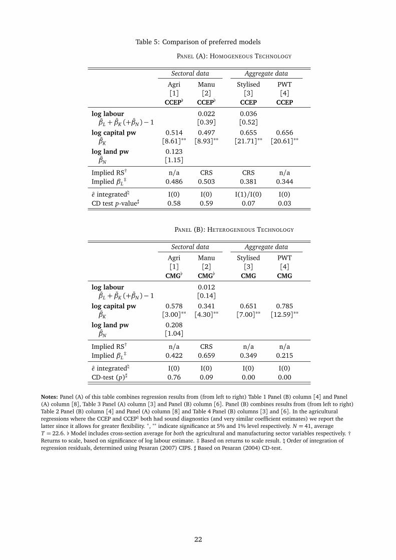
Table 5: Comparison of preferred models

PANEL (A): HOMOGENEOUS TECHNOLOGY

Sectoral data Aggregate data

Agri Manu Stylised PWT[1] [2] [3] [4]

CCEP[ CCEP[ CCEP CCEP

log labour 0.022 0.036βL + βK (+βN )− 1 [0.39] [0.52]

log capital pw 0.514 0.497 0.655 0.656βK [8.61]∗∗ [8.93]∗∗ [21.71]∗∗ [20.61]∗∗

log land pw 0.123βN [1.15]

Implied RS† n/a CRS CRS n/aImplied βL

‡ 0.486 0.503 0.381 0.344

e integrated\ I(0) I(0) I(1)/I(0) I(0)CD test p-value] 0.58 0.59 0.07 0.03

PANEL (B): HETEROGENEOUS TECHNOLOGY

Sectoral data Aggregate data

Agri Manu Stylised PWT[1] [2] [3] [4]

CMG[ CMG[ CMG CMG

log labour 0.012βL + βK (+βN )− 1 [0.14]

log capital pw 0.578 0.341 0.651 0.785βK [3.00]∗∗ [4.30]∗∗ [7.00]∗∗ [12.59]∗∗

log land pw 0.208βN [1.04]

Implied RS† n/a CRS n/a n/aImplied βL

‡ 0.422 0.659 0.349 0.215

e integrated\ I(0) I(0) I(0) I(0)CD-test (p)] 0.76 0.09 0.00 0.00

Notes: Panel (A) of this table combines regression results from (from left to right) Table 1 Panel (B) column [4] and Panel(A) column [8], Table 3 Panel (A) column [3] and Panel (B) column [6]. Panel (B) combines results from (from left to right)Table 2 Panel (B) column [4] and Panel (A) column [8] and Table 4 Panel (B) columns [3] and [6]. In the agriculturalregressions where the CCEP and CCEP\ both had sound diagnostics (and very similar coefficient estimates) we report thelatter since it allows for greater flexibility. ∗, ∗∗ indicate significance at 5% and 1% level respectively. N = 41, averageT = 22.6. [ Model includes cross-section average for both the agricultural and manufacturing sector variables respectively. †Returns to scale, based on significance of log labour estimate. ‡ Based on returns to scale result. \ Order of integration ofregression residuals, determined using Pesaran (2007) CIPS. ] Based on Pesaran (2004) CD-test.

22

APPENDIX

A-1 Data construction and descriptives

We use a total of four datasets in our empirical analysis, comprising data for agriculture and manufacturing

(Crego et al., 1998; UNIDO, 2004; FAO, 2007), an ‘aggregated dataset’ where the labour, output and

capital stock values for the two sectors are added up, and finally a Penn World Table (PWT 6.2) dataset

(Heston et al., 2006) for comparative purposes. It is important to stress that the former three datasets

differ significantly in their construction from the latter, primarily in the choice of exchange rates and

deflation: the former use international (US$-LCU) exchange rates for the year 1990, whereas the Penn

World Table dataset comprises Purchasing Power Parity (PPP) adjusted International Dollars taking the

year 2000 as the comparative base. The former thus put an emphasis on traded goods, whereas the latter

are generally perceived to account better for non-tradables and service. Provided that all monetary values

making up the variables used in each regression are comparable (across countries, times), and given that

the comparison of sectoral and aggregated data with the PWT is for illustrative purposes, we do not feel

there is an issue in presenting results from these two conceptually different datasets.

In all cases the results present are for matched observations across datasets: the four datasets are identical

in terms of countries and time-periods — we prefer this arrangement for direct comparison despite the

fact that more observations are available for individual data sources, which may improve the robustness

of empirical estimates. We provide details on the sample makeup in Table A-I. The next two subsections

describe data construction. Descriptive statistics for all variables in the empirical analysis are presented in

Table A-II.

Table A-I: Descriptive statistics: Sample makeup for all datasets

# WBCODE COUNTRY OBS # WBCODE COUNTRY OBS

1 AUS Australia 20 22 JPN Japan 282 AUT Austria 22 23 KEN Kenya 293 BEL Belgium-Luxembourg 22 24 KOR South Korea 294 CAN Canada 30 25 LKA Sri Lanka 175 CHL Chile 20 26 MDG Madagascar 206 COL Colombia 26 27 MLT Malta 237 CRI Costa Rica 10 28 MUS Mauritius 168 CYP Cyprus 18 29 MWI Malawi 239 DNK Denmark 26 30 NLD Netherlands 23

10 EGY Egypt 24 31 NOR Norway 2211 FIN Finland 28 32 NZL New Zealand 1912 FRA France 23 33 PAK Pakistan 2413 GBR United Kingdom 22 34 PHL Philippines 2414 GRC Greece 28 35 PRT Portugal 2015 GTM Guatemala 19 36 SWE Sweden 2316 IDN Indonesia 22 37 TUN Tunisia 1717 IND India 29 38 USA United States 2318 IRL Ireland 23 39 VEN Venezuela 1919 IRN Iran 25 40 ZAF South Africa 2620 ISL Iceland 20 41 ZWE Zimbabwe 2521 ITA Italy 21 Total 928

23

Table A-II: Descriptive statistics

AGRICULTURE DATA MANUFACTURING DATA

PANEL (A): VARIABLES IN UNTRANSFORMED LEVEL TERMS

Variable mean median std. dev. min. max. Variable mean median std. dev. min. max.Output 1.74E+10 5.91E+09 2.95E+10 3.54E+07 2.24E+11 Output 7.47E+10 8.31E+09 2.07E+11 7.20E+06 1.43E+12Labour 9.51E+06 1.21E+06 3.45E+07 3.00E+03 2.33E+08 Labour 1.73E+06 4.75E+05 3.42E+06 9.56E+03 1.97E+07Capital 6.42E+10 1.01E+10 1.45E+11 2.90E+07 8.64E+11 Capital 1.33E+11 1.91E+10 2.97E+11 1.41E+07 1.81E+12Land 1.73E+07 3.50E+06 4.06E+07 6.00E+03 1.91E+08

in logarithmsOutput 22.369 22.500 1.737 17.382 26.134 Output 22.812 22.840 2.292 15.790 27.991Labour 13.984 14.006 2.011 8.006 19.267 Labour 13.081 13.072 1.653 9.166 16.794Capital 22.933 23.037 2.276 17.183 27.485 Capital 23.619 23.675 2.269 16.462 28.222Land 15.089 15.068 1.986 8.700 19.066

in growth ratesOutput 1.75% 1.94% 10.36% -41.54% 53.86% Output 4.45% 3.83% 10.09% -40.91% 84.23%Labour -0.63% 0.00% 3.00% -28.77% 13.35% Labour 1.96% 1.13% 6.83% -38.84% 78.12%Capital 1.89% 1.25% 3.61% -5.13% 31.40% Capital 4.84% 3.62% 4.97% -5.10% 53.03%Land 0.06% 0.00% 2.17% -23.06% 13.57%

PANEL (B): VARIABLES IN PER WORKER TERMS

Variable mean median std. dev. min. max. Variable mean median std. dev. min. max.Output 12,615.6 6,419.6 13,130.6 44.2 57,891.3 Output 26,898.2 20,212.6 22,071.3 753.0 101,933.8Capital 51,847.1 9,661.9 63,427.8 13.1 222,396.5 Capital 63,080.3 42,543.9 64,355.0 1,475.5 449,763.4Land 9.57 2.94 20.25 0.29 110.00

in logarithmsOutput 8.385 8.767 1.817 3.788 10.966 Output 9.731 9.914 1.084 6.624 11.532Capital 8.950 9.176 2.694 2.573 12.312 Capital 10.538 10.658 1.083 7.297 13.016Land 1.105 1.078 1.404 -1.244 4.701

in growth ratesOutput 2.33% 2.52% 10.49% -43.67% 55.98% Output 2.51% 2.48% 9.00% -66.95% 73.01%Capital 2.47% 2.00% 4.17% -7.83% 31.12% Capital 2.90% 2.91% 6.59% -71.65% 42.44%Land 0.70% 0.50% 3.40% -18.37% 28.77%

AGGREGATED DATA PENN WORLD TABLE DATA

PANEL (A): VARIABLES IN UNTRANSFORMED LEVEL TERMS

Variable mean median std. dev. min. max. Variable mean median std. dev. min. max.Output 9.22E+10 1.69E+10 2.31E+11 1.14E+08 1.55E+12 Output 4.24E+11 1.27E+11 1.01E+12 1.34E+09 7.98E+12Labour 1.12E+07 2.31E+06 3.55E+07 2.23E+04 2.40E+08 Labour 5.05E+07 1.30E+07 1.19E+08 2.12E+05 8.54E+08Capital 1.97E+11 2.79E+10 4.31E+11 1.02E+08 2.25E+12 Capital 1.21E+12 3.25E+11 2.93E+12 3.30E+09 2.27E+13

in logarithmsOutput 23.470 23.553 2.016 18.552 28.069 Output 25.423 25.564 1.716 21.018 29.708Labour 14.640 14.653 1.736 10.011 19.297 Labour 16.469 16.380 1.627 12.266 20.565Capital 24.078 24.052 2.213 18.438 28.442 Capital 26.359 26.506 1.801 21.918 30.753

in growth ratesOutput 3.17% 3.15% 7.37% -33.87% 42.14% Output 4.00% 4.00% 4.96% -37.12% 26.63%Labour 0.19% 0.49% 2.56% -11.39% 19.30% Labour 1.56% 1.43% 1.14% -1.87% 4.82%Capital 3.57% 2.73% 3.62% -5.00% 25.14% Capital 4.60% 4.19% 2.84% -1.30% 16.43%

PANEL (B): VARIABLES IN PER WORKER TERMS

Variable mean median std. dev. min. max. Variable mean median std. dev. min. max.in levelsOutput 19,327.1 10,736.2 19,174.0 72.5 76,031.1 Output 11,396.7 10,308.1 8,162.3 594.3 31,074.1Capital 49,187.4 22,087.4 55,406.5 52.7 236,312.1 Capital 36,832.4 32,026.3 31,668.2 660.8 136,891.2

in logarithmsOutput 8.830 9.281 1.845 4.284 11.239 Output 8.945 9.241 1.016 6.387 10.344Capital 9.438 10.003 2.191 3.964 12.373 Capital 9.868 10.374 1.365 6.493 11.827

in growth ratesOutput 2.95% 3.30% 7.04% -31.02% 44.49% Output 2.44% 2.57% 4.96% -41.22% 23.19%Capital 3.38% 3.14% 3.74% -18.43% 22.16% Capital 3.04% 2.77% 2.87% -4.23% 14.26%

Notes: We report the descriptive statistics for value-added (in US$1990 or PPP I$2000), labour (headcount), capital stock(same monetary values as VA in each respective dataset) and land (in hectare) for the full regression sample(n= 928; N = 41).

24

A-1.1 Sectoral and aggregated data

Investment data Data for agricultural and manufacturing investment (AgSEInv, MfgSEInv) in constant

1990 LCU, the US$-LCU exchange rate (Ex Rate, see comment below) as well as sector-specific deflators

(AgDef, TotDef) were taken from Crego et al. (1998).17 Note that Crego et al. (1998) also provide capital

stock data, which they produced through their own calculations from the investment data. Following

Martin and Mitra (2002) we believe the use of a single year exchange rate is preferrable to the use of

annual ones in the construction of real output (see next paragraph) and capital stock (see below).

Output data For manufacturing we use data on aggregate GDP in current LCU and the share of GDP

in manufacturing from the World Bank World Development Indicators (WDI) (World Bank, 2008). For

agriculture we use agricultural value-added in current LCU from the same source. We prefer the latter

over the share of GDP in agriculture for data coverage reasons (in theory coverage should be the same,

but it is not). The two sectoral value-added series are then deflated using the Crego et al. (1998) sectoral

deflator for agriculture and the total economy deflator for manufacturing, before we use the 1990 US$-

LCU exchange rates to make them comparable across countries.

Note that the currencies used in the Crego et al. (1998) data differ from those applied in the WDI data for

a number of European countries due to the adoption of the Euro: for the latter we therefore need to use

an alternative 1990 US$-LCU exchange rate for these economies.18

Labour data For agriculture we adopt the variable ‘economically active population in agriculture’ from

the FAO’s PopSTAT (FAO, 2007). Manufacturing labour is taken from UNIDO’s INDSTAT (UNIDO, 2004).

Additional data The land variable is taken from ResourceSTAT and represents arable and permanent

crop land (originally in 1000 hectare) (FAO, 2007). For the robustness checks (results available on re-

quest): the livestock variable is constructed from the data for asses (donkeys), buffalos, camels, cattle,

chickens, ducks, horses, mules, pigs, sheep & goats and turkeys in the ‘Live animals’ section of ProdSTAT.

Following convention we use the below formula to convert the numbers for individual animal species into

the livestock variable:

livestock= 1.1∗camels+ buffalos+ horses+mules+ 0.8∗cattle+ 0.8∗asses

+0.2∗pigs+ 0.1∗(sheep+goats)+ 0.01∗(chickens+ducks+turkeys)

The fertilizer variable is taken from the ‘Fertilizers archive’ of ResourceSTAT and represents agricultural

fertilizer consumed in metric tons, which includes ‘crude’ and ‘manufactured’ fertilizers. For human cap-

ital we employ years of schooling attained in the population aged 25 and above from Barro and Lee

(2001).

17Data is available in excel format on the World Bank website at http://go.worldbank.org/FS3FXW7461. All data dis-cussed in this appendix are linked at http://sites.google.com/site/medevecon/devecondata. Stata code for empiricalestimators and tests is available from SSC: pescadf, xtmg, xtcd.

18In detail, we apply exchange rates of 1.210246384 for AUT, 1.207133927 for BEL, 1.55504706 for FIN, 1.204635181 forFRA, 2.149653527 for GRC, 1.302645017 for IRL, 1.616114954 for ITA, 1.210203555 for NLD and 1.406350856 for PRT. SeeTable A-I for country codes.

25

Capital stock We construct capital stock in agriculture and manufacturing by applying the perpetual

inventory method described in detail in Klenow and Rodriguez-Clare (1997b) using the investment data

from Crego et al. (1998), which is transformed into US$ by application of the 1990 US$-LCU exchange

rate. For the construction of sectoral base year capital stock we employ average sector value-added growth

rates g j (using the deflated sectoral value-added data), the average sectoral investment to value-added

ratio (I/Y ) j and an assumed depreciation rate of 5% to construct

�

K

Y

�

0 j=

IYj

g j + 0.05

for sector j. This ratio is then multiplied by sectoral value-added in the base year to yield K0 j . Note that

the method deviates from that discussed in Klenow and Rodriguez-Clare (1997b) as they use per capita

GDP in their computations and therefore need to account for population growth in the construction of the

base year capital stock.

Aggregated data We combine the agriculture and manufacturing data to produce a stylised ‘aggregate

economy’: for labour we simply add up the headcount, for the monetary representations of output and

capital stock we can do so as well. We are afforded this ability to simply add up variables for the two

sectors by the efforts of Crego et al. (1998), who have built the first large panel dataset providing data on

investment in agriculture for a long timespan.

A-1.2 Penn World Table data

As a means of comparison we also provide production function estimates using data from PWT version 6.2.

We adopt real per capita GDP in International $ Laspeyeres (rgdpl) as measure for output and construct

capital stock using investment data (derived from the investment share in real GDP, ki, and the output

variable, rgdpl) in the perpetual inventory method described above, adopting again 5% depreciation (this

time we need to use the data on population from PWT, pop, to compute the average annual population

growth rate).

26

TECHNICAL APPENDIX

TA-1 Time-series properties of the data

Table TA-I: Second generation panel unit root tests

PANEL (A): AGRICULTURE DATA

Variables in levels Variables in growth rates

log VA pw log Labour log Cap pw VA pw Labour Cap pwlags Ztbar (p) Ztbar (p) Ztbar (p) lags Ztbar (p) Ztbar (p) Ztbar (p)

0 -0.662 (.25) 7.869 (1.00) 7.182 (1.00) 0 -16.230 (.00) -2.829 (.00) -1.550 (.06)1 -0.326 (.37) 5.392 (1.00) 3.871 (1.00) 1 -9.960 (.00) 3.394 (1.00) -0.359 (.36)2 2.911 (1.00) 7.550 (1.00) 5.490 (1.00) 2 -4.970 (.00) 5.639 (1.00) 4.161 (1.00)3 4.817 (1.00) 9.859 (1.00) 5.417 (1.00) 3 -1.474 (.07) 6.238 (1.00) 5.171 (1.00)

Land pw Land pwlags Ztbar (p) lags Ztbar (p)

0 9.432 (1.00) 0 -9.704 (.00)1 7.223 (1.00) 1 -3.433 (.00)2 6.069 (1.00) 2 1.324 (.91)3 3.266 (1.00) 3 3.132 (1.00)

PANEL (B): MANUFACTURING DATA

Variables in levels Variables in growth rates

log VA pw log Labour log Cap pw VA pw Labour Cap pwlags Ztbar (p) Ztbar (p) Ztbar (p) lags Ztbar (p) Ztbar (p) Ztbar (p)

0 0.903 (.82) 2.539 (.99) 1.668 (.95) 0 -18.029 (.00) -11.824 (.00) -9.259 (.00)1 2.631 (1.00) 1.971 (.98) 0.667 (.75) 1 -8.603 (.00) -6.586 (.00) -4.928 (.00)2 2.513 (.99) 4.240 (1.00) 2.060 (.98) 2 -3.585 (.00) -3.700 (.00) -2.263 (.01)3 4.022 (1.00) 4.066 (1.00) 3.240 (1.00) 3 -1.059 (.14) -0.176 (.43) 0.847 (.80)

PANEL (C): AGGREGATED DATA

Variables in levels Variables in growth rates

log VA pw log Labour log Cap pw VA pw Labour Cap pwlags Ztbar (p) Ztbar (p) Ztbar (p) lags Ztbar (p) Ztbar (p) Ztbar (p)

0 2.558 (.99) 6.950 (1.00) 5.920 (1.00) 0 -15.283 (.00) -5.625 (.00) -4.489 (.00)1 3.112 (1.00) 4.292 (1.00) 3.668 (1.00) 1 -8.185 (.00) -2.324 (.01) -1.073 (.14)2 5.190 (1.00) 4.906 (1.00) 4.177 (1.00) 2 -3.429 (.00) 0.035 (.51) 1.154 (.88)3 5.361 (1.00) 5.131 (1.00) 4.307 (1.00) 3 -0.640 (.26) 2.637 (1.00) 3.472 (1.00)

PANEL (D): PENN WORLD TABLE DATA

Variables in levels Variables in growth rates

log VA pw log Labour log Cap pw VA pw Labour Cap pwlags Ztbar (p) Ztbar (p) Ztbar (p) lags Ztbar (p) Ztbar (p) Ztbar (p)

0 4.544 (1.00) -1.069 (.14) 2.802 (1.00) 0 -14.287 (.00) 0.711 (.76) -4.690 (.00)1 6.126 (1.00) 7.647 (1.00) 6.097 (1.00) 1 -6.603 (.00) -1.977 (.02) -2.437 (.01)2 6.581 (1.00) 7.215 (1.00) 7.215 (1.00) 2 -4.112 (.00) 1.784 (.96) -1.801 (.04)3 7.772 (1.00) 6.475 (1.00) 7.576 (1.00) 3 -1.050 (.15) 2.205 (.99) -0.468 (.32)

Notes: We report test statistics and p-values for the Pesaran (2007) CIPS panel unit root test of the variables in our fourdatasets. In all cases we use N = 41, n= 928 for the levels data.

i

TA-2 Cross-section dependence in the data

Table TA-II: Cross-section correlation analysis

Variables in levels Variables in first differences

AGRICULTURE DATA ρ |ρ| CD CDZ ρ |ρ| CD CDZ

log VA pw 0.41 0.57 57.65 74.45 0.05 0.23 6.57 6.59(p) (.00) (.00) (.00) (.00)

log Labour -0.01 0.76 -1.10 0.45 0.12 0.52 14.50 22.60(p) (.27) (.65) (.00) (.00)

log Cap pw 0.41 0.72 56.06 97.01 0.08 0.40 9.09 11.26(p) (.00) (.00) (.00) (.00)

log Land pw 0.02 0.72 2.90 3.49 0.04 0.28 4.96 5.67(p) (.00) (.00) (.00) (.00)

MANUFACTURING DATA ρ |ρ| CD CDZ ρ |ρ| CD CDZ

log VA pw 0.43 0.63 66.34 84.24 0.05 0.21 6.27 6.49(p) (.00) (.00) (.00) (.00)

log Labour 0.26 0.60 38.19 54.53 0.14 0.25 17.82 18.98(p) (.00) (.00) (.00) (.00)

log Cap pw 0.61 0.77 86.11 136.03 0.07 0.22 8.22 9.04(p) (.00) (.00) (.00) (.00)

AGGREGATED DATA ρ |ρ| CD CDZ ρ |ρ| CD CDZ

log VA pw 0.61 0.69 83.57 118.17 0.08 0.23 10.65 11.23(p) (.00) (.00) (.00) (.00)

log Labour 0.01 0.72 1.36 6.42 0.06 0.31 8.24 9.47(p) (.18) (.00) (.00) (.00)

log Cap pw 0.76 0.85 97.16 188.46 0.07 0.29 7.99 9.81(p) (.00) (.00) (.00) (.00)

PENN WORLD TABLE DATA ρ |ρ| CD CDZ ρ |ρ| CD CDZ

log VA pw 0.72 0.74 111.55 170.81 0.14 0.20 21.89 19.07(p) (.00) (.00) (.00) (.00)

log Labour 0.95 0.95 149.58 298.19 0.11 0.38 16.80 17.57(p) (.00) (.00) (.00) (.00)

log Cap pw 0.76 0.86 116.84 219.82 0.26 0.38 39.69 38.66(p) (.00) (.00) (.00) (.00)

Notes: In all cases we use N = 41, n= 928 for the levels data. We report the average correlation coefficient across theN(N − 1) variable series ρ, as well as the average absolute correlation coefficient |ρ|. CD and CDZ are formal cross-sectioncorrelation tests introduced by Pesaran (2004) and Moscone and Tosetti (2009). Under the H0 of cross-section independenceboth statistics are asymptotically standard normal. We investigated two further tests introduced by Moscone and Tosetti(2009), namely CD-LM and CD-ABS, which yield the same conclusions as the tests presented (detailed results available onrequest).

ii

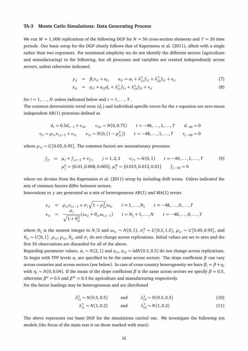
TA-3 Monte Carlo Simulations: Data Generating Process

We run M = 1,000 replications of the following DGP for N = 50 cross-section elements and T = 30 time

periods. Our basic setup for the DGP closely follows that of Kapetanios et al. (2011), albeit with a single

rather than two regressors. For notational simplicity we do not identify the different sectors (agriculture

and manufacturing) in the following, but all processes and variables are created independently across

sectors, unless otherwise indicated.

yi t = βi x i t + ui t ui t = αi +λyi1 f1t +λ

yi2 f2t + εi t (7)

x i t = ai1+ ai2dt +λxi1 f1t +λ

xi3 f3t + vi t (8)

for i = 1, . . . , N unless indicated below and t = 1, . . . , T .

The common deterministic trend term (dt) and individual-specific errors for the x-equation are zero-mean

independent AR(1) processes defined as

dt = 0.5dt−1+υd t υd t ∼ N(0,0.75) t =−48, . . . , 1, . . . , T d−49 = 0

vi t = ρvi vi,t−1+υi t υi t ∼ N(0, (1−ρ2vi)) t =−48, . . . , 1, . . . , T vi,−49 = 0

where ρvi ∼ U[0.05,0.95]. The common factors are nonstationary processes

f j t = µ j + f j,t−1+υ f t j = 1,2, 3 υ f t ∼ N(0,1) t =−49, . . . , 1, . . . , T (9)

µaj = {0.01,0.008, 0.005}, µm

j = {0.015,0.012, 0.01} f j,−50 = 0

where we deviate from the Kapetanios et al. (2011) setup by including drift terms. Unless indicated the

sets of common factors differ between sectors.

Innovations to y are generated as a mix of heterogeneous AR(1) and MA(1) errors

εi t = ρiεεi,t−1+σi

Æ

1−ρ2iεωi t i = 1, . . . , N1 t =−48, . . . , 0, . . . , T

εi t =σi

p

1+ θ2iε

(ωi t + θiεωi,t−1) i = N1+ 1, . . . , N t =−48, . . . , 0, . . . , T

where N1 is the nearest integer to N/2 and ωi t ∼ N(0,1), σ2i ∼ U[0.5,1.5], ρiε ∼ U[0.05,0.95], and

θiε ∼ U[0,1]. ρvi , ρiε, θiε and σi do not change across replications. Initial values are set to zero and the

first 50 observations are discarded for all of the above.

Regarding parameter values, αi ∼ N(2,1) and ai1, ai2 ∼ iidN(0.5, 0.5) do not change across replications.

To begin with TFP levels αi are specified to be the same across sectors. The slope coefficient β can vary

across countries and across sectors (see below). In case of cross-country heterogeneity we have βi = β+ηi

with ηi ∼ N(0, 0.04). If the mean of the slope coefficient β is the same across sectors we specify β = 0.5,

otherwise βa = 0.5 and βm = 0.3 for agriculture and manufacturing respectively.

For the factor loadings may be heterogeneous and are distributed

λxi1 ∼ N(0.5, 0.5) and λx

i3 ∼ N(0.5, 0.5) (10)

λyi1 ∼ N(1, 0.2) and λ

yi2 ∼ N(1, 0.2) (11)

The above represents our basis DGP for the simulations carried out. We investigate the following ten

models (the focus of the main text is on those marked with stars):

iii

(1) Cross-country homogeneity (β) and no factors. We set all λi to zero such that x and y are stationary

and cross-sectionally independent; technology is the same across countries and sectors.

(2) As Model (1) but now we have heterogeneous β across countries.

(3) As Model (2) but with substantially larger heterogeneity in TFP levels across countries.

(4) Æ As Model (2) but with TFP levels in manufacturing are now 1.5 times those in agriculture. We

keep this feature for the remainder of setups.

(5) This sees the introduction of common factors ( f2t and f3t) albeit with homogeneous factor loadings

across countries. Both factors and loadings are independent across sectors. The absence of f1t means

there is no endogeneity problem.

(6) Æ As Model (5) but now we have factor loading heterogeneity across countries.

(7) As Model (6) but with factor-overlap between x and y equations: f1t is contained in both of these,

inducing endogeneity in a sectoral regression.

(8) Æ As Model (7) but slope coefficients now differ across countries and sectors — for the latter we

specify βmi = 1− βa

i .

(9) As Model (8) except we now have independent slope coefficients across sectors with means βm = 0.3

and βa = 0.5.

(10) Æ As Model (9) but we now have the same factor f1t contained in y and x-equations of both sectors,

although with differential (and independent) factor loadings.

Models (1) to (4) analyse a homogeneous parameter world without common factors, where aggregation

should lead to no problems for estimation. Models (5) to (7) show what happens when factors are in-

troduced. Models (8) and (9) introduce parameter heterogeneity across sectors and Model (10) adds

factor-overlap between sectors (on top of overlap across variables within sector).

iv

TA-4 Monte Carlo simulations: overview of results

Figure TA-I: Box plots — Simulation results

Notes: We present box plots for the M = 1, 000 estimates using various estimators under 4 DGP setups. In all cases the truecoefficient is subtracted from the estimates, such that the plots are centred around zero.The estimators are as follows: ‘CMG Agri’ and ‘CMG Manu’ — Pesaran (2006) CMG regressions on the sector-level data;Weighted — this is not an estimator but the weighted average β asa

i + βmsm

i with β j the mean sectoral slope coefficient and s j

the sectoral share of total output; the remaining four estimators use the aggregated data: OLS — pooled OLS with T − 1 yeardummies; 2FE — OLS with country and time dummies; FD — OLS with variables in first differences (incl. time dummies);CMG — Pesaran (2006) CMG. We omit the results for the Pesaran and Smith (1995) MG estimator as these are very impreciseand would counter the readability of the graphs. The MC setups are described in detail in Section TA-3 of the Appendix.

v

TA-5 Monte Carlo simulations: detailed results

Table TA-III: Simulation results

MODEL 1 MODEL 2mean median ste• ste[ mean median ste• ste[

CMG Agri 0.4999 0.4990 0.0318 0.0324 CMG Agri 0.5007 0.4996 0.0425 0.0424CMG Manu 0.4999 0.4990 0.0318 0.0324 CMG Manu 0.5007 0.4996 0.0425 0.0424Weighted 0.5000 0.5000 0.0000 Weighted 0.5007 0.4998 0.0289POLS 0.5054 0.5064 0.0462 0.0298 POLS 0.5058 0.5065 0.0572 0.03042FE 0.5002 0.5005 0.0248 0.0226 2FE 0.5014 0.5007 0.0392 0.0232FD 0.5000 0.5007 0.0295 0.0257 FD 0.5014 0.5014 0.0441 0.0262CCEP 0.4996 0.4997 0.0292 0.0271 CCEP 0.5008 0.5001 0.0424 0.0276MG 0.4993 0.4987 0.0276 0.0283 MG 0.5001 0.4993 0.0389 0.0399CMG 0.4999 0.4990 0.0318 0.0324 CMG 0.5007 0.4996 0.0425 0.0424

MODEL 3 MODEL 4mean median ste• ste[ mean median ste• ste[

CMG Agri 0.4999 0.4990 0.0318 0.0324 CMG Agri 0.4999 0.4990 0.0318 0.0324CMG Manu 0.4999 0.4990 0.0318 0.0324 CMG Manu 0.4999 0.4990 0.0318 0.0324Weighted 0.5000 0.5000 0.0000 Weighted 0.5000 0.5000 0.0000POLS 0.5310 0.5280 0.1968 0.1128 POLS 0.5119 0.5112 0.0593 0.03652FE 0.5002 0.5005 0.0248 0.0226 2FE 0.5002 0.5005 0.0248 0.0226FD 0.5000 0.5007 0.0295 0.0257 FD 0.5000 0.5007 0.0295 0.0257CCEP 0.4996 0.4997 0.0292 0.0271 CCEP 0.4996 0.4997 0.0292 0.0271MG 0.4993 0.4987 0.0276 0.0283 MG 0.4993 0.4987 0.0276 0.0283CMG 0.4999 0.4990 0.0318 0.0324 CMG 0.4999 0.4990 0.0318 0.0324

MODEL 5 MODEL 6mean median ste• ste[ mean median ste• ste[

CMG Agri 0.4993 0.4987 0.0299 0.0298 CMG Agri 0.5005 0.5002 0.0238 0.0233CMG Manu 0.5000 0.5014 0.0311 0.0321 CMG Manu 0.4994 0.5004 0.0253 0.0246Weighted 0.5000 0.5000 0.0000 Weighted 0.5000 0.5000 0.0000POLS 0.4936 0.4936 0.0753 0.0432 POLS 0.4558 0.4669 0.1059 0.01972FE 0.4563 0.4571 0.0331 0.0266 2FE 0.4382 0.4450 0.0588 0.0176FD 0.4427 0.4416 0.0418 0.0268 FD 0.4181 0.4224 0.0517 0.0219CCEP 0.4516 0.4502 0.0327 0.0278 CCEP 0.4231 0.4326 0.0522 0.0186MG 0.4663 0.4687 0.3257 0.0369 MG 0.4305 0.4333 0.1816 0.0496CMG 0.4498 0.4497 0.0362 0.0379 CMG 0.4161 0.4226 0.0516 0.0342

MODEL 7 MODEL 8mean median ste• ste[ mean median ste• ste[

CMG Agri 0.5000 0.4998 0.0448 0.0436 CMG Agri 0.5009 0.5020 0.0528 0.0520CMG Manu 0.4979 0.4972 0.0454 0.0445 CMG Manu 0.4986 0.4978 0.0550 0.0528Weighted 0.5000 0.5000 0.0000 Weighted 0.5007 0.4998 0.0289POLS 0.4405 0.4469 0.1212 0.0236 POLS 0.4459 0.4452 0.1299 0.02482FE 0.4143 0.4161 0.0700 0.0210 2FE 0.4217 0.4234 0.0807 0.0220FD 0.4027 0.4011 0.0541 0.0238 FD 0.4106 0.4073 0.0635 0.0245CCEP 0.3956 0.3987 0.0619 0.0227 CCEP 0.4040 0.4047 0.0702 0.0233MG 0.6759 0.6585 0.2510 0.0782 MG 0.6826 0.6644 0.2532 0.0828CMG 0.3897 0.3928 0.0584 0.0496 CMG 0.3985 0.3976 0.0650 0.0560

MODEL 9 MODEL 10mean median ste• ste[ mean median ste• ste[

CMG Agri 0.5009 0.5020 0.0528 0.0520 CMG Agri 0.5009 0.5020 0.0528 0.0520CMG Manu 0.2961 0.2972 0.0543 0.0526 CMG Manu 0.2961 0.2972 0.0543 0.0526Weighted 0.3924 0.3928 0.0391 Weighted 0.3939 0.3946 0.0391POLS 0.3383 0.3388 0.1324 0.0246 POLS 0.3400 0.3415 0.1322 0.02462FE 0.3151 0.3127 0.0814 0.0217 2FE 0.3163 0.3144 0.0816 0.0217FD 0.3074 0.3053 0.0625 0.0242 FD 0.3086 0.3071 0.0626 0.0242CCEP 0.2963 0.2973 0.0666 0.0229 CCEP 0.2976 0.2986 0.0667 0.0229MG 0.5793 0.5562 0.2558 0.0814 MG 0.5796 0.5561 0.2558 0.0815CMG 0.2956 0.2962 0.0625 0.0543 CMG 0.2970 0.2976 0.0627 0.0544

Notes: See Section TA-3 in the Appendix for details on the estimators and the DGP in each of the experiments.ste• marks the empirical standard error and ste[ the mean standard error from 1,000 replications. ‘CMG Agri’ and ‘CMGManu’ employ the sector-level data, ‘Weighted’ calculates the aggregate slope coefficient based on the size (output) and slopeof the respective sector, the remaining six estimators use the aggregated data.

vi

TA-6 Additional tables and figures

Table TA-IV: Pooled regression models (HC-augmented)

PANEL (A): UNRESTRICTED RETURNS TO SCALE

Agriculture Manufacturing

[1] [2] [3] [4] [5] [6] [7] [8] [9] [10]POLS 2FE CCEP CCEP[ FD POLS 2FE CCEP CCEP[ FD

log labour -0.079 -0.151 -0.457 -0.557 -0.085 0.005 0.029 0.121 -0.048 0.162[11.71]∗∗ [4.35]∗∗ [1.54] [1.46] [1.46] [0.62] [0.88] [1.91] [0.47] [4.62]∗∗

log capital pw 0.471 0.671 0.554 0.676 0.595 0.692 0.851 0.533 0.446 0.654[61.84]∗∗ [27.20]∗∗ [4.51]∗∗ [4.32]∗∗ [12.60]∗∗ [44.38]∗∗ [22.14]∗∗ [8.00]∗∗ [4.52]∗∗ [14.56]∗∗

log land pw 0.018 -0.020 -0.154 -0.174 0.111[1.17] [0.48] [0.56] [0.50] [1.14]

Education 0.241 0.087 0.007 -0.068 0.101 0.226 -0.006 0.152 -0.017 0.095[9.95]∗∗ [3.12]∗∗ [0.07] [0.40] [1.30] [11.91]∗∗ [0.21] [2.04]∗ [0.16] [1.53]

Educationˆ2 -0.010 -0.007 -0.003 0.005 -0.006 -0.009 0.002 -0.006 -0.004 -0.005[4.73]∗∗ [4.15]∗∗ [0.49] [0.50] [1.23] [6.22]∗∗ [1.39] [1.32] [0.66] [1.10]

Implied RS† CRS CRS CRS CRS IRS CRS CRS CRS IRSImplied βL

‡ 0.529 0.329 0.446 0.324 0.321 0.308 0.149 0.467 0.508e integrated\ I(1) I(1) I(0) I(1)/I(0) I(0) I(1) I(1) I(0) I(0) I(0)CD test p-value] 0.11 0.09 0.14 0.21 0.00 0.87 0.18 0.58 0.84 0.00Mean Education 5.82 5.82 5.82 5.82 5.94 5.82 5.82 5.82 5.82 5.94Returns to Edu 13.3% 0.7% -2.9% -0.7% 3.0% 12.3% 1.9% 8.5% -6.6% 4.1%

[t-statistic][ [15.71]∗∗ [0.50] [0.68] [0.11] [0.78] [19.88]∗∗ [1.30] [3.11]∗∗ [1.56] [1.54]R-squared 0.91 0.57 1.00 1.00 - 0.91 0.57 1.00 1.00 -Observations 830 830 830 775 793 860 860 860 775 817

PANEL (B): CONSTANT RETURNS TO SCALE IMPOSED

Agriculture Manufacturing

[1] [2] [3] [4] [5] [6] [7] [8] [9] [10]POLS 2FE CCEP CCEP[ FD POLS 2FE CCEP CCEP[ FD

log capital pw 0.502 0.720 0.592 0.709 0.611 0.695 0.839 0.472 0.463 0.558[59.09]∗∗ [33.18]∗∗ [5.32]∗∗ [5.08]∗∗ [13.29]∗∗ [49.18]∗∗ [24.30]∗∗ [8.87]∗∗ [5.59]∗∗ [13.85]∗∗

log land pw 0.014 0.078 0.144 0.122 0.124[0.71] [2.23]∗ [0.99] [0.69] [1.27]

Education 0.278 0.069 -0.003 -0.031 0.107 0.226 0.014 0.234 0.036 0.220[11.54]∗∗ [2.48]∗ [0.03] [0.23] [1.38] [11.80]∗∗ [0.71] [3.67]∗∗ [0.38] [3.91]∗∗

Educationˆ2 -0.012 -0.005 0.000 0.002 -0.006 -0.009 0.001 -0.010 -0.007 -0.010[6.17]∗∗ [3.19]∗∗ [0.06] [0.28] [1.26] [6.11]∗∗ [0.98] [2.55]∗ [1.22] [2.41]∗

Implied βL‡ 0.498 0.202 0.408 0.291 0.389 0.305 0.162 0.528 0.537 0.443

Mean Education 5.82 5.82 5.82 5.82 5.94 5.82 5.82 5.82 5.82 5.94Returns to Edu 13.9% 0.8% -0.7% -0.3% 3.4% 12.3% 2.7% 11.7% -4.3% 10.5%

[t-statistic]♠ [16.25]∗∗ [0.52] [0.18] [0.07] [0.90] [20.20]∗∗ [2.30]∗ [5.25]∗∗ [1.18] [4.62]∗∗

e integrated\ I(1) I(1) I(0) I(1)/I(0) I(0) I(1) I(1) I(0) I(1)/I(0) I(0)CD test p-value] 0.29 0.23 0.07 0.23 0.00 0.88 0.04 0.08 0.02 0.00R-squared 0.91 0.57 1.00 1.00 - 0.91 0.57 1.00 1.00 -Observations 830 830 830 775 793 860 860 860 775 817

Notes: We include our proxy for education in levels and as a squared term. Returns to Education are computed from thesample mean (E) as βE +2βE2 E where βE and βE2 are the coefficients on the levels and squared education terms respectively.♠ computed via the delta-method. For more details see Notes of Table 1 of the main text.

vii

Table TA-V: Heterogeneous Manufacturing models (HC-augmented)

PANEL (A): UNRESTRICTED PANEL (B): CRS IMPOSED

[1] [2] [3] [4] [5] [6]MG FDMG CMG MG FDMG CMG

log labour -0.305 -0.293 0.097[1.20] [1.50] [0.62]

log capital pw 0.059 0.144 0.426 0.352 0.347 0.386[0.22] [0.74] [3.73]∗∗ [3.25]∗∗ [3.66]∗∗ [3.95]∗∗

Education -0.478 0.237 1.248 -0.228 0.085 0.668[1.02] [0.81] [2.66]∗ [0.62] [0.29] [2.43]∗

Education squared 0.050 0.011 -0.098 0.005 -0.019 -0.042[1.38] [0.35] [2.67]∗ [0.13] [0.67] [1.95]

country trend/drift 0.016 0.020 0.008 0.013[1.55] [2.44]∗ [1.16] [2.23]∗

reject CRS (10%) 38% 8% 38%Implied βL

‡ n/a 0.857 0.574 0.648 0.653 0.614Mean Education 5.82 5.91 5.82 5.87 5.94 5.87Returns to Edu -6.3% -1.3% 10.9% -6.2% -2.1% 11.9%[t-statistic][ [1.01] [0.25] [1.89] [1.00] [0.47] [1.70]panel-t Labour 4.49∗∗ -2.51∗ 1.81panel-t Capital 0.30 -0.25 8.62∗∗ 7.52∗∗ 5.48∗∗ 10.19∗∗

panel-t Edu 2.08∗ 0.93 3.58∗∗ 3.08∗∗ 0.88 3.38∗∗

panel-t Eduˆ2 1.93 -0.91 3.31∗∗ 2.47∗ 0.97 2.67∗∗

panel-t trend/drift 12.59∗∗ 6.41∗∗ 13.89 7.05sign. trends (10%) 15 9 17 7e integrated\ I(0) I(0) I(0) I(0) I(0) I(0)abs correl. coeff. 0.21 0.22 0.22 0.22 0.22 0.22CD-test (p)] 0.00 0.00 0.71 0.00 0.00 0.27Obs (N) 775 (37) 732 (37) 775 (37) 775 (37) 732 (37) 775 (37)

Notes: All averaged coefficients presented are robust means across i. [ The returns to educationand associated t-statistics are based on a two-step procedure: first the country-specific meaneducation value (Ei) is used to compute βi,E + 2βi,E2 Ei to yield the country-specific returns toeducation. The reported value then represents the robust mean of these N country estimates, s.t.the t-statistic should be interpreted in the same fashion as that for the regressors, namely as a testwhether the average parameter is statistically different from zero, following Pesaran and Smith(1995). For other details see Notes for Tables 2 (main text) and TA-IV above.

viii

Table TA-VI: Aggregate & PWT data: Pooled models (HC-augmented)

PANEL (A): UNRESTRICTED RETURNS

Aggregated data Penn World Table data

[1] [2] [3] [4] [5] [6] [7] [8]POLS 2FE CCEP FD POLS 2FE CCEP FD

log labour -0.001 -0.058 0.566 0.083 0.040 -0.064 -0.193 -0.032[0.14] [1.97]∗ [4.13]∗∗ [2.50]∗ [8.99]∗∗ [3.27]∗∗ [1.49] [1.11]

log capital pw 0.662 0.782 0.677 0.766 0.725 0.680 0.601 0.676[97.95]∗∗ [31.50]∗∗ [7.25]∗∗ [25.24]∗∗ [72.79]∗∗ [24.79]∗∗ [9.12]∗∗ [18.96]∗∗

Education 0.243 -0.004 0.086 0.065 0.041 0.043 0.032 0.103[16.97]∗∗ [0.15] [1.24] [1.22] [3.42]∗∗ [2.86]∗∗ [0.80] [3.41]∗∗

Education squared -0.010 0.003 -0.007 -0.003 -0.001 -0.002 -0.002 -0.006[8.05]∗∗ [1.82] [1.57] [0.77] [1.77] [2.97]∗∗ [0.83] [2.94]∗∗

Implied RS† CRS DRS CRS CRS CRS DRS CRS CRSImplied βL

‡ 0.337 0.160 0.890 0.318 0.315 0.256 0.206 0.292Mean Education 5.824 5.824 5.824 5.885 5.822 5.822 5.822 5.883Returns to Edu 12.9% 2.5% 1.0% 3.4% 2.4% 1.9% 0.9% 3.3%[t-statistic][ [22.35]∗∗ [1.68] [0.37] [1.40] [6.82]∗∗ [2.02]∗ [0.56] [2.26]∗

e integrated\ I(1) I(1) I(0) I(0) I(1) I(1) I(0) I(1)/I(0)CD test p-value] 0.00 0.02 0.59 0.00 0.34 0.22 0.01 0.00R-squared 0.98 0.87 1.00 - 0.97 0.78 1.00 -Observations 775 775 775 732 769 769 769 726

PANEL (B): CONSTANT RETURNS TO SCALE IMPOSED

Aggregated data Penn World Table data

[1] [2] [3] [4] [5] [6] [7] [8]POLS 2FE CCEP FD POLS 2FE CCEP FD

log capital pw 0.662 0.798 0.485 0.744 0.694 0.706 0.611 0.691[102.10]∗∗ [35.45]∗∗ [7.03]∗∗ [25.48]∗∗ [73.08]∗∗ [27.73]∗∗ [10.05]∗∗ [21.13]∗∗

Education 0.243 -0.016 0.210 0.111 0.043 0.037 0.016 0.092[16.98]∗∗ [0.62] [3.00]∗∗ [2.21]∗ [3.30]∗∗ [2.44]∗ [0.48] [3.22]∗∗

Education squared -0.010 0.004 -0.013 -0.005 -0.001 -0.002 -0.002 -0.006[8.17]∗∗ [2.75]∗∗ [2.92]∗∗ [1.37] [0.97] [2.12]∗ [0.95] [2.79]∗∗

Constant 1.586 1.843[21.62]∗∗ [20.44]∗∗

Implied βL‡ 0.338 0.203 0.515 0.256 0.306 0.294 0.390 0.309

Mean Education 5.824 5.824 5.824 5.885 5.822 5.824 5.824 5.883Returns to Edu 12.9% 2.6% 6.5% 5.8% 3.3% 2.0% -0.6% 2.7%[t-statistic][ [22.41]∗∗ [1.68] [2.56]∗∗ [2.56]∗∗ [8.62]∗∗ [1.99]∗ [0.42] [1.98]∗

e integrated\ I(1) I(1) I(0) I(0) I(1) I(1) I(0) I(0)CD test p-value] 0.00 0.00 0.65 0.00 0.25 0.57 0.02 0.00R-squared 0.98 0.86 1.00 0.97 0.78 1.00Observations 775 775 775 732 769 769 769 726

Notes: We include our proxy for education in levels and as a squared term. Returns to Education are computed from thesample mean (E) as βE +2βE2 E where βE and βE2 are the coefficients on the levels and squared education terms respectively.[ computed via the delta-method. For more details see Notes for Tables 3 (in the main text) and (for the education variables)TA-IV above.

ix

Table TA-VII: Aggregate & PWT data: Heterogeneous models with HC

PANEL (A): UNRESTRICTED RETURNS TO SCALE

Aggregated data Penn World Table data

[1] [2] [3] [4] [5] [6]MG FDMG CMG MG FDMG CMG

log labour -0.066 0.269 -0.428 -1.609 -2.478 -1.324[0.16] [0.57] [1.22] [1.97] [3.76]∗∗ [2.79]∗∗

log capital pw -0.070 -0.021 0.453 0.963 1.245 1.122[0.26] [0.07] [2.47]∗ [4.44]∗∗ [5.99]∗∗ [5.52]∗∗

Education 0.601 0.637 0.489 0.123 0.004 -0.012[1.29] [1.75] [0.98] [0.52] [0.02] [0.05]

Education squared -0.089 -0.065 -0.063 -0.002 0.004 -0.001[1.76] [1.70] [1.48] [0.11] [0.25] [0.03]

country trend/drift 0.005 0.005 0.021 0.008[0.33] [0.29] [2.25]∗ [0.77]

Mean Education 5.72 5.84 5.72 5.72 5.84 5.72Returns to edu -7.1% -3.2% -11.1% -4.5% 0.5% 1.3%[t-statistic][ [1.33] [0.65] [1.24] [1.33] [0.18] [0.43]Implied RS† CRS CRS CRS CRS DRS DRSImplied βL

‡ n/a n/a 0.547 n/a n/a n/areject CRS (10%) 38% 3% 19% 38% 18% 33%panel-t Labour -1.77 0.16 -1.42 -6.37∗∗ -5.60∗∗ -7.30∗∗

panel-t Capital 0.58 0.94 2.79∗∗ 15.62∗∗ 13.48∗∗ 14.39∗∗

panel-t Edu 0.26 1.21 0.86 0.89 0.23 0.68panel-t Edu ˆ2 -1.07 -1.87 -1.26 -1.55 -0.35 -0.72panel-t trends 14.73∗∗ 10.93∗∗ 11.09∗∗ 5.83∗∗

# sign. trends 18 13 18 4e integrated\ I(0) I(0) I(0) I(0) I(0) I(0)abs correl.coeff. 0.24 0.24 0.22 0.23 0.24 0.22CD-test (p)] 7.23(.00) 7.88(.00) -0.50(.61) 7.59.00) 9.29.00) 0.98(.33)

PANEL (B): CRS IMPOSED

Aggregated data Penn World Table data

[1] [2] [3] [4] [5] [6]MG FDMG CMG MG FDMG CMG

log capital pw 0.093 0.151 0.528 0.779 1.052 0.906[0.49] [0.90] [4.90]∗∗ [5.75]∗∗ [6.43]∗∗ [5.86]∗∗

Education 0.075 0.260 0.683 -0.215 -0.134 0.089[0.18] [0.99] [1.73] [1.25] [0.84] [0.42]

Education squared -0.023 -0.023 -0.075 0.013 0.014 -0.023[0.65] [0.89] [1.57] [0.82] [1.13] [1.16]

country trend/drift 0.017 0.015 -0.001 -0.010[1.96] [1.33] [0.21] [2.08]∗

Implied βL‡ n/a n/a 0.472 0.221 n/a 0.094

Mean Education 5.79 5.84 5.79 5.79 5.84 5.79Returns to edu -9.3% -4.0% 3.2% -1.4% 0.3% -0.2%[t-statistic][ -1.34 -0.88 0.50 0.50 0.16 0.05panel-t Capital 2.96∗∗ 1.84 7.63∗∗ 16.24∗∗ 11.99∗∗ 15.70∗∗

panel-t Edu -2.05∗ 1.97∗ 3.78∗∗ -1.80 -1.23 0.74panel-t Edu ˆ2 0.79 -2.77∗∗ -3.83∗∗ 1.20 0.96 -1.11panel-t trends 15.65∗∗ 12.21∗∗ 11.57∗∗ 7.84∗∗

# sign. trends 15 13 15 14e integrated\ I(0) I(0) I(0) I(0) I(0) I(0)abs correl.coeff. 0.24 0.24 0.23 0.26 0.24 0.22CD-test (p)] 8.05(.00) 8.59(.00) 0.11(.92) 9.75(.00) 10.84(.00) 3.12(.00)

Notes: All averaged coefficients presented are robust means across i. [ The returns toeducation and associated t-statistics are based on a two-step procedure: first thecountry-specific mean education value (Ei) is used to compute βi,E + 2βi,E2 Ei to yieldthe country-specific returns to education. The reported value then represents therobust mean of these N country estimates, s.t. the t-statistic should be interpreted inthe same fashion as that for the regressors, namely as a test whether the averageparameter is statistically different from zero, following Pesaran and Smith (1995). Forother details see Notes for Tables 2 (in the main text) and TA-V above.

x

Table TA-VIII: Alternative dynamic panel estimators

PANEL (A): AGRICULTURE

Dynamic FE PMG CPMG? DGMM SGMM

[1] [2] [3] [4] [5] [6] [7] [8] [9] [10] [11] [12]EC [yt−1] -0.293 -0.312 -0.300 -0.460 -0.459 -0.624 -0.466 -0.482 -0.503 -0.455 -1.087 -0.432

[11.80]∗∗ [12.43]∗∗ [11.91]∗∗ [10.63]** [9.34]∗∗ [14.29]∗∗ [10.44]∗∗ [10.06]∗∗ [9.74]∗∗ [9.34]∗∗ [2.60]∗∗ [5.38]∗∗

capital pw 0.672 0.684 0.582 0.652 0.714 0.036 0.132 0.501 0.464 0.530 1.135 0.776[12.47]∗∗ [12.69]∗∗ [7.50]∗∗ [20.16]∗∗ [18.52]∗∗ [0.57] [3.01]∗∗ [10.78]∗∗ [11.05]∗∗ [10.83]∗∗ [2.85]∗∗ [12.59]∗∗

land pw 0.124 0.121 0.135 0.136 0.367 0.867 0.361 0.247 0.494 0.228 0.083 -0.247[1.30] [1.29] [1.45] [2.90]∗∗ [6.43]∗∗ [8.27]∗∗ [8.05]∗∗ [5.03]∗∗ [8.95]∗∗ [4.73]∗∗ [0.35] [1.17]

trend(s)† 0.001 0.008 0.012[1.59] [3.36]∗∗ [12.26]∗∗

Constant 0.667 0.679 0.896 1.072 0.644 4.273 3.084 1.545 1.402 1.298 0.714[5.03]∗∗ [4.75]∗∗ [4.58]∗∗ [10.48]∗∗ [7.53]∗∗ [13.11]∗∗ [10.27]∗∗ [10.38]∗∗ [9.69]∗∗ [9.94]∗∗ [4.21]∗∗

lags [trends]‡ 1 2 1 [l-r] 1 2 1 [s-r] 1 [l-r] 1 2 1 i: 2-3 i: 2-3impl. labour 0.328 0.316 0.418 0.212 -0.081 0.098 0.507 0.253 0.042 0.242 -0.135 0.224obs 894 857 894 894 857 894 894 894 857 872 857 894

PANEL (B): MANUFACTURING

Dynamic FE PMG CPMG? DGMM SGMM

[1] [2] [3] [4] [5] [6] [7] [8] [9] [10] [11] [12]EC [yt−1] -0.196 -0.195 -0.195 -0.219 -0.181 -0.543 -0.214 -0.245 -0.194 -0.272 -2.196 -0.041

[9.40]∗∗ [9.16]∗∗ [9.31]∗∗ [6.59]∗∗ [5.97]∗∗ [4.04]∗∗ [4.13]∗∗ [7.16]∗∗ [6.45]∗∗ [7.33]∗∗ [0.72] [0.65]capital pw 0.711 0.708 0.637 1.016 1.044 0.298 1.379 0.598 1.264 0.505 1.866 -1.515

[12.96]∗∗ [12.34]∗∗ [6.85]∗∗ [29.64]∗∗ [33.09]∗∗ [5.34]∗∗ [26.80]∗∗ [11.58]∗∗ [22.28]∗∗ [9.47]∗∗ [3.25]∗∗ [0.40]trend(s)† 0.001 0.001 -0.010

[1.00] [0.24] [6.77]∗∗

Constant 0.452 0.456 0.588 -0.212 -0.228 3.493 -0.977 0.225 -0.434 0.372 1.042[3.87]∗∗ [3.73]∗∗ [3.29]∗∗ [5.43]∗∗ [4.95]∗∗ [3.87]∗∗ [4.18]∗∗ [5.68]∗∗ [5.77]∗∗ [6.48]∗∗ [1.80]

lags [trends]‡ 1 2 1 [l-r] 1 2 1 [s-r] 1 [l-r] 1 2 1 i: 2-3 i: 2-3impl. labour 0.289 0.292 0.363 -0.016 -0.044 0.702 -0.379 0.402 -0.264 0.495 -0.866 2.515obs 902 880 902 902 880 902 902 902 880 879 880 902

PANEL (C): AGGREGATED DATA

Dynamic FE PMG CPMG? DGMM SGMM

[1] [2] [3] [4] [5] [6] [7] [8] [9] [10] [11] [12]EC [yt−1] -0.172 -0.176 -0.173 -0.279 -0.277 -0.429 -0.284 -0.292 -0.294 -0.317 -0.380 -0.243

[8.59]∗∗ [8.39]∗∗ [8.59]∗∗ [6.89]∗∗ [7.25]∗∗ [9.55]∗∗ [6.72]∗∗ [6.98]∗∗ [7.38]∗∗ [7.48]∗∗ [0.71] [4.21]∗∗

capital pw 0.705 0.709 0.668 0.974 1.015 0.128 0.899 0.891 0.949 0.905 0.271 0.896[15.25]∗∗ [14.65]∗∗ [8.17]∗∗ [36.86]∗∗ [37.38]∗∗ [1.90] [21.11]∗∗ [24.84]** [24.92]∗∗ [27.54]∗∗ [0.27] [22.80]∗∗

trend(s)† 0.000 0.011 0.004[0.54] [6.07]∗∗ [2.42]∗

Constant 0.390 0.393 0.446 -0.100 -0.200 3.061 0.082 -0.062 -0.169 -0.145 0.120[4.96]∗∗ [4.62]∗∗ [3.42]∗∗ [3.73]∗∗ [5.18]∗∗ [9.30]∗∗ [4.20]∗∗ [2.53]∗ [4.97]∗∗ [4.58]∗∗ [1.44]

lags [trends]‡ 1 2 1 [l-r] 1 2 1 [s-r] 1 [l-r] 1 2 1 i: 2-3 i: 2-3impl. labour 0.295 0.292 0.332 0.026 -0.015 0.872 0.102 0.109 0.051 0.095 0.729 0.104obs 879 836 879 879 836 879 879 879 836 879 836 879

PANEL (D): PENN WORLD TABLE DATA

Dynamic FE PMG CPMG? DGMM SGMM

[1] [2] [3] [4] [5] [6] [7] [8] [9] [10] [11] [12]EC [yt−1] -0.098 -0.101 -0.107 -0.333 -0.138 -0.567 -0.392 -0.338 -0.081 -0.347 0.835 0.031

[5.82]∗∗ [6.01]∗∗ [6.22]∗∗ [6.70]∗∗ [4.37]∗∗ [12.63]∗∗ [7.88]∗∗ [6.63]∗∗ [2.56]∗ [8.24]∗∗ [1.07] [0.49]capital pw 0.538 0.553 0.356 0.923 0.916 0.698 0.652 0.903 -0.125 0.731 0.604 0.863

[8.14]∗∗ [8.66]∗∗ [3.44]∗∗ [130.34]∗∗ [71.72]∗∗ [65.10]∗∗ [67.96]∗∗ [52.90]∗∗ [1.81] [86.83]∗∗ [0.60] [1.88]trend(s)† 0.001 0.002 0.006

[2.44]∗ [2.57]∗ [19.84]∗∗

Constant 0.363 0.360 0.567 -0.122 -0.020 1.085 0.935 -0.071 0.456 0.504 0.010[5.38]∗∗ [5.29]∗∗ [5.28]∗∗ [4.44]∗∗ [1.63] [13.05]∗∗ [7.79]∗∗ [3.47]∗∗ [2.99]∗∗ [8.29]∗∗ [0.07]

lags [trends]‡ 1 2 1 [l-r] 1 2 1 [s-r] 1 [l-r] 1 2 1 i: 2-3 i: 2-3impl. labour 0.462 0.447 0.645 0.077 0.084 0.302 0.349 0.097 1.125 0.270 0.396 0.137obs 914 904 914 914 904 914 914 904 873 904 914

Notes: We report the long-run coefficients on capital per worker (and in the agriculture equations also land per worker). EC[yt−1] refers to the Error-Correction term (speed of adjustment parameter) with the exception of Models [11] and [12],where we report the coefficient on yt−1 — conceptually, these are the same, however in the latter we do not impose commonfactor restrictions like in all of the former models. Note that in the PMG and CPMG models the ECM term is heterogeneousacross countries, while in the Dynamic FE and GMM models these are common across i. † In model [6] we includeheterogeneous trend terms, whereas in [7] a common trend is assumed (i.e. linear TFP is part of cointegrating vector). ‡ ‘lags’indicates the lag-length of first differenced RHS variables included, with the exception of Models [11] and [12]: here ‘i:’refers to the lags (levels in [11], levels and differences in [12] used as instruments. ? In the models in [8] and [9] thecross-section averages are only included for the long-run variables, whereas in the model in [10] cross-section averages forthe first-differenced dependent and independent variables (short-run) are also included. Note that in the agriculture equationfor Model [10] we drop CRI (n= 7) as otherwise no convergence would occur.

xi