Embed Size (px)
Citation preview

Credit Market Failure and Macroeconomics
Joachim Jungherr
Thesis submitted for assessment with a view to obtaining the degree of Doctor of Economics of the European University Institute
Florence, November 2013

Jungherr, Joachim (2013), Credit market failure and macroeconomics European University Institute
DOI: 10.2870/929
European University Institute Department of Economics
Credit Market Failure and Macroeconomics
Joachim Jungherr
Thesis submitted for assessment with a view to obtaining the degree of Doctor of Economics of the European University Institute
Examining Board Prof. Árpád Ábrahám, European University Institute (Supervisor) Prof. Hugo A. Hopenhayn, UCLA Prof. Ramon Marimon, European University Institute Prof. Vincenzo Quadrini, University of Southern California
© Joachim Jungherr, 2013 No part of this thesis may be copied, reproduced or transmitted without prior permission of the author
Jungherr, Joachim (2013), Credit market failure and macroeconomics European University Institute
DOI: 10.2870/929

Jungherr, Joachim (2013), Credit market failure and macroeconomics European University Institute
DOI: 10.2870/929
ii
Abstract
This thesis aims to contribute to our understanding of the relationship betweenmarket failure on capital markets and macroeconomic outcomes in various forms. Thenotion of credit markets as a frictionsless veil over real economic activity has proven tobe unfruitful with respect to many questions of economic interest. To name only a fewexamples, in the absence of nancial frictions there is no dierence between internaland external nancing, no trade-o between equity and debt, and there is no reasonfor banks to exist. In order to correctly identify and address the policy needs whichmight arise from credit market failure, we need to learn more about the fundamentalconditions which give rise to the nancial contracts and institutions observed in reality.
The rst chapter of this thesis focuses on the phenomenon of the publicly tradedrm with its separation of ownership and control. I show how a time-varying misalign-ment of incentives of rm managers and investors can have important consequences foraggregate business uctuations. In particular, a rise in idiosyncratic rm-level uncer-tainty may result in an economy-wide increase in the default rate on corporate bondstogether with a drop in measured rm productivity and output.
Bank transparency is the topic of the second chapter. In this model, banks arespecial because the product they are selling is superior information about investmentopportunities. Intransparent balance sheets turn this public good into a marketableprivate commodity. In the absence of policy intervention, bank competition resultsin complete bank opacity and a high degree of aggregate uncertainty for households.Mandatory disclosure rules can improve upon the market outcome.
The third chapter is joint work with David Strauss. It focuses on the consequencesof credit market failure for development and growth. We show that capital marketimperfections may give rise to a poverty trap associated with permanent productiv-ity dierences across countries. Key to this phenomenon is a sorting reversal in thematching between human capital and heterogeneous production sectors.
Jungherr, Joachim (2013), Credit market failure and macroeconomics European University Institute
DOI: 10.2870/929

iii
Acknowledgements
This PhD thesis is the product of four rich and exciting years during which I learned
more than I had reason to hope for at the outset. Push the envelope. Watch it bend.
The guidance and ever-encouraging support from my adviser Árpád Ábrahám were
invaluable for me. Especially at times when both of us where unsure what I was up to.
I would like to think that I got contaminated by his enthusiasm for economics. I would
also like to thank Vincenzo Quadrini for making my stay at the University of Southern
California possible. I beneted a lot from our discussions and I took many memories
home with me from this journey to the New World. Ramon Marimon was kind enough
to join the team when it was already late in the game. Many thanks for that.
During three years of my PhD studies, I was supported by a scholarship from the
German Academic Exchange Service (DAAD), which also contributed to my research
visit at the University of Southern California in Los Angeles.
The joint part of this thesis owes much to my co-author David Strauss. Generally, I
consider myself as very lucky having spent these four years at the European University
Institute. The lively and inspiring atmosphere in Villa San Paolo and the solidarity
among that bunch of would-be economists it is packed with are probably unique and
certainly a gift which I enjoyed a lot.
Without the superb work of the administrative sta and the many other non-
academic members of the EUI, the whole Institute would have fallen apart a long time
ago. Therefore, I need to thank Jessica, Lucia, Marcia, Giuseppe, Loredana, Sonia and
everybody else who keeps this social engine running day by day.
But I would not have been able to fully appreciate the academic amenities of the
Doctoral Programme without the time spent with the IUE Calcio team on rain-soaked
mud pitches all over orentine suburbia. I have to express my gratitude to the Squadra
Fantastica for uncountable memorable moments and a life beyond my desk in VSP.
Along the journey of these last four years, I had the privilege to share the road with
many persons, some of which became very close friends along the way. Every single one
of them has made this experience richer. I would not have wanted to undertake this
journey alone. My deepest gratitude to all of them.
My family both in Germany as well as in Florence has given me the strength and
the condence which I could not have obtained anywhere else.
Barcelona, September 23rd, 2013
Jungherr, Joachim (2013), Credit market failure and macroeconomics European University Institute
DOI: 10.2870/929

iv
Meinen Eltern
Jungherr, Joachim (2013), Credit market failure and macroeconomics European University Institute
DOI: 10.2870/929
Contents
Preface . . . . . . . . . . . . . . . . . . . . . . . . . . . . . . . . . . . . . . . . . . vii
Chapter 1 Capital Structure, Uncertainty, and Macroeconomic Fluctuations 1
1.1 Introduction . . . . . . . . . . . . . . . . . . . . . . . . . . . . . . . . . . . . 1
1.2 Model Setup . . . . . . . . . . . . . . . . . . . . . . . . . . . . . . . . . . . . 10
1.2.1 Firms . . . . . . . . . . . . . . . . . . . . . . . . . . . . . . . . . . . 11
1.2.2 Managers . . . . . . . . . . . . . . . . . . . . . . . . . . . . . . . . . 11
1.2.3 Households . . . . . . . . . . . . . . . . . . . . . . . . . . . . . . . . 12
1.2.4 Timing . . . . . . . . . . . . . . . . . . . . . . . . . . . . . . . . . . . 12
1.3 Perfect Information . . . . . . . . . . . . . . . . . . . . . . . . . . . . . . . . 13
1.3.1 Households . . . . . . . . . . . . . . . . . . . . . . . . . . . . . . . . 13
1.3.2 Optimal Contract . . . . . . . . . . . . . . . . . . . . . . . . . . . . . 14
1.3.3 Characterization . . . . . . . . . . . . . . . . . . . . . . . . . . . . . 16
1.4 Financial Frictions . . . . . . . . . . . . . . . . . . . . . . . . . . . . . . . . 17
1.4.1 Optimal Contract . . . . . . . . . . . . . . . . . . . . . . . . . . . . . 18
1.4.2 Capital Structure . . . . . . . . . . . . . . . . . . . . . . . . . . . . . 27
1.4.3 Households . . . . . . . . . . . . . . . . . . . . . . . . . . . . . . . . 30
1.4.4 Characterization . . . . . . . . . . . . . . . . . . . . . . . . . . . . . 31
1.5 Quantitative Analysis . . . . . . . . . . . . . . . . . . . . . . . . . . . . . . . 32
1.5.1 Parametrization . . . . . . . . . . . . . . . . . . . . . . . . . . . . . . 33
1.5.2 Optimal Contract . . . . . . . . . . . . . . . . . . . . . . . . . . . . . 36
1.5.3 Uncertainty and Financial Markets . . . . . . . . . . . . . . . . . . . 38
1.5.4 Business Cycle Analysis . . . . . . . . . . . . . . . . . . . . . . . . . 40
1.6 Discussion . . . . . . . . . . . . . . . . . . . . . . . . . . . . . . . . . . . . . 45
Appendix A Proofs and Derivations . . . . . . . . . . . . . . . . . . . . . . . . . 47
Appendix B Model Solution and Simulation . . . . . . . . . . . . . . . . . . . . 53
v
Jungherr, Joachim (2013), Credit market failure and macroeconomics European University Institute
DOI: 10.2870/929

vi CONTENTS
Chapter 2 Bank Opacity and Endogenous Uncertainty 61
2.1 Introduction . . . . . . . . . . . . . . . . . . . . . . . . . . . . . . . . . . . . 61
2.2 Model Setup . . . . . . . . . . . . . . . . . . . . . . . . . . . . . . . . . . . . 67
2.2.1 Households . . . . . . . . . . . . . . . . . . . . . . . . . . . . . . . . 67
2.2.2 Banks . . . . . . . . . . . . . . . . . . . . . . . . . . . . . . . . . . . 67
2.2.3 Projects and Information . . . . . . . . . . . . . . . . . . . . . . . . . 68
2.2.4 Timing . . . . . . . . . . . . . . . . . . . . . . . . . . . . . . . . . . . 69
2.3 Equilibrium . . . . . . . . . . . . . . . . . . . . . . . . . . . . . . . . . . . . 69
2.3.1 Households . . . . . . . . . . . . . . . . . . . . . . . . . . . . . . . . 70
2.3.2 Banks: Exogenous Transparency . . . . . . . . . . . . . . . . . . . . 71
2.3.3 Banks: Endogenous Transparency . . . . . . . . . . . . . . . . . . . . 74
2.4 Optimal Opacity . . . . . . . . . . . . . . . . . . . . . . . . . . . . . . . . . 76
2.5 Discussion . . . . . . . . . . . . . . . . . . . . . . . . . . . . . . . . . . . . . 78
Appendix A Proofs and Derivations . . . . . . . . . . . . . . . . . . . . . . . . . 80
Chapter 3 Why Does Misallocation Persist? 91
3.1 Introduction . . . . . . . . . . . . . . . . . . . . . . . . . . . . . . . . . . . . 91
3.2 Model Setup . . . . . . . . . . . . . . . . . . . . . . . . . . . . . . . . . . . . 98
3.2.1 Agents . . . . . . . . . . . . . . . . . . . . . . . . . . . . . . . . . . . 98
3.2.2 Production . . . . . . . . . . . . . . . . . . . . . . . . . . . . . . . . 98
3.2.3 Final Good . . . . . . . . . . . . . . . . . . . . . . . . . . . . . . . . 99
3.2.4 Labor Market . . . . . . . . . . . . . . . . . . . . . . . . . . . . . . . 100
3.2.5 Timing . . . . . . . . . . . . . . . . . . . . . . . . . . . . . . . . . . . 100
3.3 Ecient Allocation . . . . . . . . . . . . . . . . . . . . . . . . . . . . . . . . 100
3.3.1 Production . . . . . . . . . . . . . . . . . . . . . . . . . . . . . . . . 101
3.3.2 Sorting . . . . . . . . . . . . . . . . . . . . . . . . . . . . . . . . . . . 102
3.3.3 Final Good . . . . . . . . . . . . . . . . . . . . . . . . . . . . . . . . 106
3.3.4 Intermediate Goods . . . . . . . . . . . . . . . . . . . . . . . . . . . . 107
3.3.5 Labor Market . . . . . . . . . . . . . . . . . . . . . . . . . . . . . . . 107
3.3.6 Dynamics . . . . . . . . . . . . . . . . . . . . . . . . . . . . . . . . . 108
3.4 Misallocation . . . . . . . . . . . . . . . . . . . . . . . . . . . . . . . . . . . 108
3.4.1 Production . . . . . . . . . . . . . . . . . . . . . . . . . . . . . . . . 109
3.4.2 Sorting . . . . . . . . . . . . . . . . . . . . . . . . . . . . . . . . . . . 109
3.4.3 Dynamics . . . . . . . . . . . . . . . . . . . . . . . . . . . . . . . . . 111
3.5 Discussion . . . . . . . . . . . . . . . . . . . . . . . . . . . . . . . . . . . . . 114
Jungherr, Joachim (2013), Credit market failure and macroeconomics European University Institute
DOI: 10.2870/929
Preface
This thesis aims to contribute to our understanding of the relationship between market
failure on capital markets and macroeconomic outcomes. The formal analysis of nancial
frictions in its current form has its roots in the literature on private information and limited
commitment. These endeavors date back until the 1970s, but the Financial Crisis of 2007-
2008 and the Great Recession have certainly added further momentum to the progress of
this research agenda. The common understanding underlying the current discussion is that
the notion of smoothly functioning credit markets has proven to be unfruitful with respect
to many questions of economic interest. To name only a few examples, in the absence of
nancial frictions there is no dierence between internal and external nancing, no trade-o
between equity and debt, and there is no reason for banks to exist. In order to correctly
identify and address the policy needs which might arise from credit market failure, we need
to learn more about the fundamental conditions which give rise to the nancial contracts and
institutions observed in reality. Capital market imperfections can arise for many dierent
reasons and can take on very dierent forms, each of which potentially yields dierent policy
recommendations. In my view, the literature has only begun to explore these possibilities
and their theoretical and practical implications both for the business cycle and economic
growth.
One example of a nancial institution which cannot be understood without the analysis
of nancial frictions is the phenomenon of the publicly traded rm with its separation of
ownership and control. The recent Financial Crisis did not hit only privately held rms
which rely on bank lending as the principal source of nancing, but also rms with access
to capital markets were considerably aected by adverse credit conditions during the crisis.
Credit spreads and default rates soared on corporate bond markets. At the same time,
companies were exposed to a particularly sharp rise in sales and growth volatility, while
measured total factor productivity (TFP) experienced the sharpest downturn of the post-
war era. In the rst chapter of this thesis, I employ an optimal contract approach to security
design and capital structure to show how an increase in rm-level uncertainty can result in
vii
Jungherr, Joachim (2013), Credit market failure and macroeconomics European University Institute
DOI: 10.2870/929
viii CREDIT MARKET FAILURE AND MACROECONOMICS
a rise of the default rate on corporate bonds together with a drop in rm productivity and
output. Key to the analysis is a misalignment of the incentives of rm management and
investors. Within a dynamic general equilibrium model, I study the impact of exogenous
variations in rm-level uncertainty on real and nancial aggregates. Uncertainty shocks of
plausible size typically cause a recession featuring a rise in default rates and a deleveraging of
the corporate sector. An important driver of the business cycle in this model are uctuations
in the Solow residual which are not caused by technology shocks, but by the time-varying
severity of agency problems.
Bank transparency is the topic of the second chapter of this thesis. What is special about
banks that makes them more opaque than non-nancial rms? What exactly are the exter-
nalities which give rise to a need for policy intervention? And what is the optimal level of
bank transparency? In this model, banks are special because the product they are selling is
superior information about investment opportunities. Intransparent balance sheets turn this
public good into a marketable private commodity. Voluntary public disclosure of informa-
tion translates into a competitive disadvantage. Bank competition results in a race to the
bottom which leads to complete bank opacity and a high degree of aggregate uncertainty
for households. Households do value public information as it reduces aggregate uncertainty,
but the market does not punish intransparent banks. Policy measures can improve upon the
market outcome by imposing minimum disclosure requirements on banks. However, com-
plete disclosure is socially undesirable as this eliminates all private incentives for banks to
acquire costly information. The social planner chooses optimal bank transparency by trading
o the benets of reducing aggregate uncertainty for households against banks' incentives
for costly information acquisition.
The third chapter of this thesis is joint work with David Strauss. It focuses on the long
term consequences of credit market failure for development and growth. Total factor produc-
tivity (TFP) accounts for the major part of cross-country dierences in per capita income.
Factor misallocation can potentially explain large TFP losses. However, existing models of
factor misallocation through credit market frictions fail to robustly generate large eects on
TFP in the long run. We propose a new mechanism to show how capital market imperfec-
tions may indeed give rise to a permanent misallocation of production factors within a given
country and permanent dierences in measured TFP across countries. In the presence of
binding credit constraints, the assignment of human capital to production sectors is com-
pletely reversed with respect to the case of ecient capital markets. Factor misallocation
may be permanent because of the possibility of a collective poverty trap which arises for low
levels of nancial development. Depending on initial conditions, a country converges over
Jungherr, Joachim (2013), Credit market failure and macroeconomics European University Institute
DOI: 10.2870/929

PREFACE ix
time to one of two dierent stable steady states characterized by dierent long-run levels
of output, capital, wages, and measured TFP. Manufacturing goods are relatively cheaper
in the high-income steady state compared to the low-income equilibrium, while the average
rm size and its variance are higher.
Jungherr, Joachim (2013), Credit market failure and macroeconomics European University Institute
DOI: 10.2870/929

x CREDIT MARKET FAILURE AND MACROECONOMICS
Jungherr, Joachim (2013), Credit market failure and macroeconomics European University Institute
DOI: 10.2870/929

Jungherr, Joachim (2013), Credit market failure and macroeconomics European University Institute
DOI: 10.2870/929

Chapter 1
Capital Structure, Uncertainty, and
Macroeconomic Fluctuations
1.1 Introduction
Capital market imperfections have been identied as a major determinant of the origin and
the severity of the Great Recession which was triggered by the Financial Crisis of 2007-2008.
The common narrative attributes a central role to borrowing constraints of privately held
rms which rely on bank loans as the principal source of nancing.1 But also rms with access
to capital markets were considerably aected by adverse credit conditions during the crisis.
The default rate on corporate bonds reached its second highest level of the post-war period
in 2009.2 Corporate bond spreads almost tripled between 2007 and 2009 (Adrian, Colla and
Shin, 2013).3 At the same time, companies were exposed to a particularly sharp rise in
sales and growth volatility4, while total factor productivity (TFP) experienced the sharpest
downturn of the post-war era (Fernald, 2012). This paper employs an optimal contract
approach to security design and capital structure to show how an increase in the severity
of nancial frictions can result in a rise of the default rate on corporate bonds together
with a drop in rm protability, measured TFP, and rm output. Key to the analysis is a
misalignment of the incentives of rm management and investors. Time-varying rm-level
1See Bernanke (2010), Duygan-Bump, Levkov and Montoriol-Garriga (2011), or Shourideh and Zetlin-Jones (2012)
2This data is provided by Giesecke, Longsta, Schaefer and Strebulaev (2013). During the 2001 U.S.recession, the default rate on corporate bonds was slightly higher than in 2009.
3Likewise, Gilchrist and Zakraj²ek (2012) document a dramatic rise in credit spreads on corporate bondmarkets during the crisis.
4See Bloom, Floetotto, Jaimovich, Saporta-Eksten and Terry (2012), or Schaal (2012).
1
Jungherr, Joachim (2013), Credit market failure and macroeconomics European University Institute
DOI: 10.2870/929
2 CHAPTER 1. CAPITAL STRUCTURE AND UNCERTAINTY
uncertainty determines the severity of this agency problem.
This paper explains the emergence of debt and equity securities as eciently designed
instruments to implement an optimal contract between investors and rm managers in an
environment subject to asymmetric information. Taking seriously the optimal design and
usage of nancing instruments at the rm level has two main advantages. First, we can be
condent to understand the most important characteristics of the economic environment to
the extent that we are able to rationalize the nancial contracts observed in reality. Standard
macroeconomic models do not perform too well in this respect, as they struggle to rationalize
common forms of rm nancing such as the prevalent use of a certain combination of equity
and bond securities by publicly traded companies. Secondly, the analysis developed below
sheds light on the role of rm-level risk in determining the severity of the agency problem
between investors and rm managers which gives rise to a non-trivial capital structure choice
between equity and debt. In times of high volatility at the rm level, rms need to reduce
their leverage in order to avoid a rise in default risk. However, reduced leverage gives rm
managers more discretion in pursuing non-prot-maximizing rm policies. The optimal
adjustment of the rm's capital structure trades o these two eects, which generally results
in some combination of higher default risk, lower rm productivity, and lower rm output.
The nancing choice of the individual rm is embedded in a dynamic general equilibrium
model subject to exogenous variations in rm-level uncertainty of plausible size. This model
features a number of empirical business cycle facts which standard macro models fail to
generate. Namely, the model replicates the countercyclical behavior of rm-level uncertainty
and corporate bond default rates. In addition, this model economy features uctuations in
the Solow residual which are not caused by technology shocks, but by the time-varying sever-
ity of agency conicts between investors and rm managers. This is an important nding, as
Chari, Kehoe and McGrattan (2007) show that variations of total factor productivity (the
eciency wedge") are a major determinant of the U.S. business cycle.5
Preview of the Model
In order to study the nancing decision of rms, I build on a standard agency theory of
the rm along the lines of Ross (1973) and others. In many situations, the incentives of
rm managers and investors are not aligned. Firm managers decide on how hard to work
5Chari, Kehoe and McGrattan (2007) conclude their article stating:
The challenging task is to develop detailed models in which primitive shocks lead to uctuationsin eciency wedges [...]."
Jungherr, Joachim (2013), Credit market failure and macroeconomics European University Institute
DOI: 10.2870/929
1.1. INTRODUCTION 3
as well as on how hard they try to make their employees work. They choose how much
rm resources to spend on the pursuit of managerial benets such as an overly pleasant
work environment or favoring friends in contracting relationships with the rm (Jensen and
Meckling, 1976). These incentive problems may even go so far as to aect the selection of
large-scale investment projects by choosing rm growth over rm protability (Jensen, 1986).
The underlying reason for this problem is asymmetric information between rm managers
and outside investors. Firm managers have the information required to take the right action
on behalf of investors but they may not have the appropriate incentives to do so.
This agency problem is modeled in a simple way. Investors want managers to exert
costly eort on their behalf. Firm managers observe the productivity state of the rm before
they choose the level of eort. Outside investors observe realized rm output but can neither
assess the true level of eort provided by the manager nor the stochastic productivity level of
the rm. Performance pay is one way for investors to provide incentives for managers. This
classical principal-agent setup is augmented with a monitoring technology as introduced by
Townsend (1979). Depending on the level of rm productivity announced by the manager,
investors can choose to pay for a thorough assessment of the company's true productivity
state which allows for a richer set of nancial contracts.
Results
The resulting optimal contract lends itself to a straightforward interpretation as a unique
combination of equity and debt nancing. Optimally, only low realizations of rm produc-
tivity are monitored. By identifying the event of monitoring as bankruptcy proceedings,
the cash ows to investors can be separated into distinct payment streams to creditors and
shareholders. Debt is a xed claim which triggers monitoring (bankruptcy) in case of default.
This notion of bankruptcy as a costly device for outsiders to acquire rm-specic informa-
tion dates back to Townsend (1979) and Gale and Hellwig (1985). According to this idea, an
important feature of bankruptcy proceedings is a transfer of rm-specic information from
insiders to outsiders. Creditors of a rm in default pay accountants and trustees to assess
the true value of the rm's assets in place in order to recover as much of the face value of
debt as possible.6 This option to verify the rm manager's announcements reduces agency
costs not only in case of actual bankruptcy, but also in all non-bankruptcy states. Conse-
6This resembles most closely the process of liquidation of a rm by a trustee according to Chapter 7of the U.S. Bankruptcy Code. However, also Chapter 11 reorganizations put the debtor under scrutiny bycreditors. Bris, Welch and Zhu (2006) estimate that the direct expenses related to Chapter 7 liquidationsand Chapter 11 reorganizations are of similar size.
Jungherr, Joachim (2013), Credit market failure and macroeconomics European University Institute
DOI: 10.2870/929
4 CHAPTER 1. CAPITAL STRUCTURE AND UNCERTAINTY
quently, by issuing non-contingent debt securities rms can limit the freedom of managers
to deviate from the prot-maximizing production plan. The downside of leverage consists of
an elevated risk to incur the costs of bankruptcy. Equity holders are the residual claimants
of the rm. Accordingly, they receive a positive dividend after all debt and wage obligations
are satised.
The result that in this model rms optimally rely on a certain combination of equity and
debt instruments to nance investment is important, because it is in line with the design and
usage of securities issued by rms in practice. Fama and French (2005) report that 26% of
the total asset growth of U.S. listed rms between 1993 and 2002 were nanced by net equity
issuance, while the growth of total liabilities accounts for 68%.7 Stock measures of nancing
sources convey a similar message. According to Fama and French (2005), the total liabilities
of their rm sample account for about two thirds of the aggregate book value of assets, while
shareholders' equity sums up to about one third of the aggregate balance sheet.8
In the model economy, corporate capital structure is determined as a trade-o between
agency costs and the risk of costly bankruptcy. Issuing debt restricts the freedom of rm
managers to deviate from prot-maximizing rm policies. This benet of debt comes at
the expense of an increased risk of costly bankruptcy. Up to this point, this model of rm
nancing is very much in line with the extensive literature on corporate capital structure.910
What is new in this analysis is the central role of uncertainty about idiosyncratic, rm-
specic characteristics. Whenever the business environment of a given rm is particularly
volatile, rm performance becomes hard to predict. This gives much room for discretion to
the rm's management and exacerbates the agency problem in question. The default risk
increases as the optimal monitoring frequency grows in an attempt to put tighter controls
on rm management. At the same time, the expected levels of rm output, measured
productivity, and return on investment implied by the optimal contract fall relative to their
perfect information counterparts.
7The remaining 6% of total rm asset growth are nanced by retained earnings. This information isbased on Table 2 in Fama and French (2005) using dSB as the measure of net equity issuance.
8While publicly traded rms are only a trivial fraction of all rms in the U.S., they account for morethan 25% of total employment (Davis, Haltiwanger, Jarmin and Miranda, 2007). Shourideh and Zetlin-Jones(2012) calculate that roughly 60% of corporate gross output is produced by publicy traded rms.
9Typically, trade-o theories of capital structure also consider interest tax shields as an additional benetof debt nancing. See also the discussion at the end of the paper in Section 1.6.
10This model of optimal corporate capital structure is also backed up by empirical evidence on the economicsignicance both of agency and bankruptcy costs. Morellec, Nikolov and Schürho (2012) and Nikolov andSchmid (2012) nd that agency costs in the manager-shareholder relationship are an important determinantof the capital structure choice of publicly traded rms. Bris, Welch and Zhu (2006) nd bankruptcy fees tobe increasing in rm size and report an empirical magnitude of about 10% of rm asset value. Dependingon rm characteristics, their estimate varies between 0% and 20%.
Jungherr, Joachim (2013), Credit market failure and macroeconomics European University Institute
DOI: 10.2870/929
1.1. INTRODUCTION 5
Various measures of rm-level uncertainty have been documented to move cyclically over
time. In particular, Bloom, Floetotto, Jaimovich, Saporta-Eksten and Terry (2012) nd
that for a given rm at time t the volatilities of shocks to total factor productivity, daily
stock returns, and sales growth are all positively correlated among each other. Apparently,
these measures capture a common underlying state of rm-level uncertainty which varies
over time.11 Furthermore, these measures of idiosyncratic rm risk display a robustly coun-
tercyclical behavior.12 The Great Recession 2007-2009 featured a particularly sharp rise in
rm-level risk.13
The causal relationship between rm-level uncertainty and the business cycle is an open
question.14 In this paper, I study within a dynamic general equilibrium model the eect of
exogenous innovations to rm-level uncertainty on the cyclical behavior of nancial and real
variables.15 I nd that an increase in uncertainty at the rm level aggravates the agency
problem between rm managers and investors, which results in a rise of default rates and
a drop in measured TFP, aggregate output, consumption, and investment. Firms reduce
leverage in times of high uncertainty, as the risk of bankruptcy increases and equity claims
gain in value at the expense of bondholders. This is consistent with the extensive empirical
literature on corporate nance which regularly nds a negative relationship between rm
risk and leverage ratios.16
Ignoring the eect of time-varying uncertainty at the micro-level results in an overestima-
tion of the signicance of other shocks to fundamentals such as aggregate technology shocks.
11Why does idiosyncratic rm risk vary over time? A change of the economic environment can aectdierent rms in vastly dierent ways. Some rms might benet from a given change in economic policy,while others suer. Accordingly, rm uncertainty could increase whenever important changes of economicpolicy are implemented or anticipated. Baker, Bloom and Davis (2013) construct an empirical measure ofeconomic policy uncertainty and nd it to be correlated with major political events such as elections, wars,the Eurozone crisis, or the U.S. debt-ceiling dispute.
12The countercyclical behavior of various measures of rm-level uncertainty has been documented fordierent countries and rm groups. See for example Campbell, Lettau, Malkiel and Xu (2001), Higson,Holly and Kattuman (2002), Higson, Holly, Kattuman and Platis (2004), Eisfeldt and Rampini (2006),Gourio (2008), Bloom (2009), Gilchrist, Sim and Zakraj²ek (2010), or Bloom et al. (2012).
13See Bloom et al. (2012) and Schaal (2012).14Bloom et al. (2012) nd no evidence that this unconditional negative correlation between idiosyncratic
uncertainty and aggregate output is merely driven by an endogenous response of uncertainty to the businesscycle. But see also Bachmann, Elstner and Sims (2010).
15Examples of models which feature an endogenous rise of idiosyncratic risk in response to aggregateshocks include Veldkamp (2005), Van Nieuwerburgh and Veldkamp (2006), and Bachmann and Moscarini(2011). A similar feedback channel from aggregate economic activity to idiosyncratic rm risk is absent frommy model, but is likely to amplify the quantitative impact of variations in uncertainty.
16See Bradley, Jarrell and Kim (1984), Friend and Lang (1988), or Korteweg (2010). Campbell and Taksler(2003) use the opposite eects of rm volatility on the value of stock and bond claims to explain the divergingperformance of equity and bond markets in the U.S. during the late 1990s.
Jungherr, Joachim (2013), Credit market failure and macroeconomics European University Institute
DOI: 10.2870/929
6 CHAPTER 1. CAPITAL STRUCTURE AND UNCERTAINTY
In this model, the Solow residual uctuates over time together with rm-level uncertainty
even in the absence of technological innovations. This is an important nding, as Chari,
Kehoe and McGrattan (2007) show that variations of total factor productivity are an impor-
tant determinant of the U.S. business cycle. Falls in measured productivity can be caused
by an endogenous increase in agency problems, as investors nd it harder to incentivize rm
managers to pursue ecient business policies in times of high uncertainty. This rationale of
declines in the Solow residual is an alternative to the idea of recurring episodes of exogenous
technological regress.
Related Literature
The key innovation of this paper consists of embedding an optimal security design approach
to rm nancing in a general equilibrium macro framework. The principal underlying ideas
originate in an earlier literature which rationalizes the design and usage of a certain com-
bination of equity and debt securities focusing on a single rm in partial equilibrium. This
research agenda can be divided into three distinct groups. One branch of literature focuses
on asymmetric information between rm managers and outside investors. Default on debt
payments triggers monitoring by outsiders, which assigns a socially valuable role to costly
bankruptcy. This approach is adopted by Chang (1993), Boyd and Smith (1998), Atkeson
and Cole (2008), and Cole (2011).17 A second line of research sees default as a mechanism
to withdraw control rights from managers in an environment of incomplete contracts. This
idea is explored by Aghion and Bolton (1992), Chang (1992), Dewatripont and Tirole (1994),
Zwiebel (1996), and Fluck (1998). A third approach views default as the termination of a
long-term nancing relationship between rm managers and outside investors, as in DeMarzo
and Sannikov (2006), Biais, Mariotti, Plantin and Rochet (2007), and DeMarzo and Fishman
(2007).18
The environment used in the model below is most closely related to the rst branch of
literature. These models all share one common feature. The agency problem between rm
managers and investors does not distort production. Firm output is an exogenous stochastic
17This literature builds on earlier contributions by Townsend (1979), Diamond (1984), and Gale andHellwig (1985). In these models, a combination of entrepreneurial (inside) equity and outside debt is optimal.Public equity held by outside investors does not have value in environments in which rm output is privateinformation of rm managers. See Townsend (1979):
The model as it stands may contribute to our understanding of closely held rms, but it cannotexplain the coexistence of publicly held shares and debt."
18Two models of the optimal design and usage of equity and debt which do not consider default are Biaisand Casamatta (1999) and Koufopoulos (2009).
Jungherr, Joachim (2013), Credit market failure and macroeconomics European University Institute
DOI: 10.2870/929
1.1. INTRODUCTION 7
process and rm managers simply decide on the payout of realized cash ows. In contrast,
I study an agency problem in which rm output will generally be ineciently low. As
the severity of the agency problem varies, so does the expected level of rm output. This
mechanism will be crucial for the result that agency conicts at the rm level can aect the
Solow residual of an economy.
Also on the macroeconomic level, rms' nancing choice between equity and debt has
been the subject of inquiry. Examples of models which analyze the interaction between
corporate capital structure and the business cycle include Levy and Hennessy (2007), Gomes
and Schmid (2010), Covas and Den Haan (2011), and Jermann and Quadrini (2012). These
models go a long way in matching empirical facts. However, the set of nancial instruments
at the disposal of agents is exogenously constrained and not derived from the economic
environment. If rms had the option to oer alternative nancial contracts to investors in
these environments, this would lead to more favorable economic outcomes. Factors which
are identied as relevant for the cyclical properties of the model will generally vary with
the exogenously imposed contract structure. As long as we do not understand the role
of nancial contracts in overcoming frictions to economic exchange, we are likely to miss
something about these underlying frictions and consequently also about their signicance
for macroeconomic uctuations. The role of idiosyncratic rm risk discussed below is one
example.
The Financial Accelerator literature, following along the lines of Bernanke and Gertler
(1989) and Bernanke, Gertler and Gilchrist (1999), proposes a strictly entrepreneurial model
of the rm and does not allow for outside equity nancing. Also, Gomes, Yaron and Zhang
(2003) show at the example of Carlstrom and Fuerst (1997) that these models tend to gen-
erate procyclical default rates which is at odds with empirical evidence. While the Financial
Accelerator literature focuses on information frictions, another line of thought follows Kiy-
otaki and Moore (1997) in putting limits to the enforceability of contracts at the center
of their analysis. These models share the exclusively entrepreneurial nature of rms and
cannot explain the occurrence of costly default in equilibrium. While Lorenzoni (2008) and
others succeed to characterize and explain the problematic nature of excessive borrowing in
a similar framework, eventual policy implications for rm nancing are put into question by
the disregard of equity nancing.19
An important contribution of this paper is the introduction of a novel propagation mech-
anism of uncertainty (or risk) shocks to the business cycle literature. At the same time, the
19For other studies of excessive borrowing in a debt-only environment, see also Brunnermeier and Sannikov(2010), or Bianchi (2011).
Jungherr, Joachim (2013), Credit market failure and macroeconomics European University Institute
DOI: 10.2870/929
8 CHAPTER 1. CAPITAL STRUCTURE AND UNCERTAINTY
general idea that idiosyncratic uncertainty may matter for aggregate outcomes is not new at
all.20 Bloom et al. (2012) show that non-convex adjustment costs to capital and labor can
give rise to a wait-and-see eect in response to temporarily elevated levels of rm-level risk.
Firms reduce investment in times of high uncertainty if they cannot costlessly reverse their
decisions afterwards. As this hampers the optimal reallocation of production factors across
plants, this can generate an endogenous decline in the Solow residual. However, Bachmann
and Bayer (2013) nd this wait-and-see eect to be quantitatively small compared to the
business cycle impact of a standard aggregate technology shock. Furthermore, Bachmann
and Bayer (2011) point out that in this environment large contractionary eects of uncer-
tainty shocks are incompatible with the procyclical behavior of the dispersion of investment
levels across rms which they document for German micro data. Also Lang (2012) nds
that the wait-and-see eect is unlikely to be strong enough such that an increase in the
dispersion of productivity shocks at the rm level can trigger an aggregate downturn.
Other studies are closer to the model outlined below in that they examine credit market
imperfections as an alternative propagation channel of innovations to the level of rm-level
uncertainty. Gilchrist, Sim and Zakraj²ek (2010) impose an exogenous contract structure
upon rms by restricting their nancing choice to equity and debt. Both security types are
subject to ad-hoc frictions. They show that uncertainty raises the cost of capital as credit
spreads rise in response to a higher risk of bankruptcy. This causes a drop in investment
with adverse consequences for optimal factor reallocation across rms and for the Solow
residual. The authors depart from the rest of the literature by assuming that rm prots
are linear in productivity (instead of being convex). This assumption facilitates to generate
countercyclical rm-level risk as shown below.21 Both Gilchrist, Sim and Zakraj²ek (2010)
and Bloom et al. (2012) rely on frictions to the ecient reallocation of production factors
across rms to generate endogenous movements of the Solow residual. Using French micro-
level data, Osotimehin (2013) nds that the eciency of factor reallocation is actually higher
during recessions than during booms. This result casts a doubt on the important procyclical
role of factor reallocation in Gilchrist, Sim and Zakraj²ek (2010) and Bloom et al. (2012).
In contrast, in the model proposed below the expected marginal product of capital will be
equalized across rms at all times.
Christiano, Motto and Rostagno (2013) build on the Financial Accelerator mechanism
20The focus of this paper lies on variations in idiosyncratic uncertainty. Recent examples of studies whichexamine shocks to aggregate uncertainty include Fernández-Villaverde, Guerrón-Quintana, Rubio-Ramírezand Uribe (2011), Basu and Bundick (2012), Leduc and Liu (2013), and Orlik and Veldkamp (2013).
21By assuming rm prots to be linear in productivity, the authors switch o the `Oi-Hartman-Abel eect'associated with procyclical idiosyncratic risk. See Oi (1961), Hartman (1972), and Abel (1983).
Jungherr, Joachim (2013), Credit market failure and macroeconomics European University Institute
DOI: 10.2870/929
1.1. INTRODUCTION 9
mentioned above and conclude that shocks to rm-level risk are the most important driver
of the business cycle. Importantly, debt is the only source of outside nancing within the
Financial Accelerator framework. But the eects of increased production risk are very dif-
ferent for the value of equity and bond claims of a given rm. Bondholders participate
only in the elevated downside risk of production outcomes, while shareholders benet from
the increase in upside risks. Excluding equity nancing from the analysis is problematic,
as this prohibits rms to sell their upside risks to investors. The result that the costs of
capital rise in uncertainty is somewhat mechanical, if only debt is considered. Furthermore,
in Christiano, Motto and Rostagno (2013) nominal rigidities and the endogenous response
of monetary policy to uncertainty shocks are crucial elements in generating realistic busi-
ness cycle co-movements. Dorofeenko, Lee and Salyer (2008) and Chugh (2012) examine
idiosyncratic uncertainty within a Financial Accelerator framework without nominal rigidi-
ties. They nd quantitatively weak results. This is consistent with the nding by Chari,
Kehoe and McGrattan (2007), that movements in the investment wedge alone are unlikely
to generate realistic business cycle properties.
Arellano, Bai and Kehoe (2012) assume exogenously incomplete markets in their study of
the role of nancial frictions in propagating innovations to rm-level risk. With Dorofeenko,
Lee and Salyer (2008), Chugh (2012), and Christiano, Motto and Rostagno (2013) they share
the focus on debt as the only source of outside rm nancing. The authors are particularly
successful in generating variations of labor demand in response to an exogenous shock to
idiosyncratic uncertainty. The underlying mechanism is very similar to the eect of a shock
to borrowing constraints as in Jermann and Quadrini (2012). Quadrini (2011) points to the
similarities between these two types of nancial shocks.
Also in Narita (2011), nancial frictions give rise to a negative role of uncertainty shocks
for the aggregate economy. The author shows that increased rm-level risk causes a rise in
the endogenous termination rate of the long-term nancial contracts introduced by DeMarzo
and Sannikov (2006). Implications for the cyclical properties of real and nancial variables
are not considered.
The endogenous movements of the Solow residual generated by the model outlined below
resemble earlier ideas on variable factor utilization developed by Burnside, Eichenbaum and
Rebelo (1993), Basu (1996), or Burnside and Eichenbaum (1996). Keeping the measured
units of aggregate capital and labor input xed, these models allow for variations in the degree
of capital utilization and labor eort which are not directly observable to econometricians.
This idea can explain movements in the Solow residual which are not caused by technology
shocks but, for instance, by innovations to government expenditures. The focus of this model
Jungherr, Joachim (2013), Credit market failure and macroeconomics European University Institute
DOI: 10.2870/929
10 CHAPTER 1. CAPITAL STRUCTURE AND UNCERTAINTY
does not lie on capital or labor, but on the quality of managerial labor as a third production
factor which is arguably hard to measure and an important determinant of the productivity
of the other two factors. Managerial eort levels do not vary over the business cycle because
of aggregate shocks, but because of variations in the severity of agency problems caused by
exogenous changes to rm-level uncertainty. The agency problem in question is based on the
corporate nance literature on optimal security design and its empirical implications can be
tested both on the micro and the macro level.
One key assumption in this model is the central role of managerial eort for the produc-
tion outcome of the entire rm. This idea is in line with empirical studies on the importance
of managerial practices for individual rm performance as documented by Bloom and Van
Reenen (2007) and Bloom, Eifert, Mahajan, McKenzie and Roberts (2013). The role of
executive managers is special because their decisions aect how ecient the other inputs to
production are used. Indirect empirical evidence on this conception of managerial activity
is provided by the studies of Baker and Hall (2004), Gabaix and Landier (2008), and Terviö
(2008), who estimate the marginal value of the labor input by top executives to increase
together with the resources under their control.
Outline
The rest of the paper is organized as follows. The model is set up in Section 1.2. Sections
1.3 and 1.4 characterize the equilibrium allocation for the frictionsless case and the case of
asymmetric information, respectively. A quantitative analysis of the model follows in Section
1.5. The paper concludes with a short discussion of future work in Section 1.6.
1.2 Model Setup
Consider a model economy with a continuum of small rms of mass unity. Each rm j ∈ [0, 1]
uses an identical constant returns to scale production technology with capital, labor, and
managerial eort as inputs. This technology is subject to both aggregate and idiosyncratic
productivity shocks. The economy is inhabited by many small and identical households of
unit mass. Households provide labor to companies and allocate their savings across rms
in order to smooth consumption over time. Each of the many small companies is run by a
single manager who exerts eort.
Jungherr, Joachim (2013), Credit market failure and macroeconomics European University Institute
DOI: 10.2870/929

1.2. MODEL SETUP 11
1.2.1 Firms
All rms produce the same homogeneous nal good which can be used either for consumption
or for investment. Firm output is given by:
yt(j) = At(j) kt(j)αk lt(j)
αlmt(j)αm ,
where kt(j) stands for the amount of capital employed in company j at time t, lt(j) measures
labor input, and mt(j) indicates managerial eort. The output elasticities of capital, labor,
and managerial eort add up to one: αk + αl + αm = 1. This functional form is chosen in
line with empirical ndings by Gabaix and Landier (2008), who estimate CEO compensation
to grow linearly in rm size indicating constant returns to scale. Firm-specic productivity
At(j) is independent and identically distributed across companies according to the cumulative
distribution function Ft(A). Its discrete support is completely characterized by the lowest
and highest realizations, A1 and An, together with ∆A = Ai − Ai−1 for i = 2, 3, ..., n. The
properties of Ft(A) vary stochastically over time with aggregate conditions.
1.2.2 Managers
There is a unit mass of rm managers. Managers have access to the constant returns to scale
production technology described above, but they do not own any savings which they could
use as capital. In order to produce, they can collect savings from households on a capital
market. Each manager can run exactly one rm. Managers provide managerial eort and
consume their wages. Their utility is given by the function:
u(ct(j),mt(j)
)= ct(j) − v
(mt(j)
),
where ct(j) and mt(j) denote consumption and labor eort provided by the manager of rm
j at time t, respectively. The function measuring the disutility of eort v : [0, 1] → R is
assumed to be increasing and strictly convex. In addition, we assume: v′(1) = −∞. If a
rm manager decides not to run a rm, she faces an outside option which generates a utility
level of u with certainty.
Firm managers live for exactly one period. At the end of each period, the current gener-
ation of managers dies and a new generation of managers is born. This assumption implies
that rms are modeled as short-term projects which can be studied independently of the
particular history of any individual rm manager.22
22The assumption of short-term nancing contracts is not uncommon in the literature. See for example
Jungherr, Joachim (2013), Credit market failure and macroeconomics European University Institute
DOI: 10.2870/929
12 CHAPTER 1. CAPITAL STRUCTURE AND UNCERTAINTY
1.2.3 Households
The household's preferences regarding an allocation of consumption Ct and labor lt over time
may be described by the function:
Et∞∑i=0
βi[U(Ct+i) − V (lt+i)
],
where Et is the expectation operator conditional on date t information, and β ∈ [0, 1] gives
the rate of time preference. The function U : [0,∞]→ R is increasing, strictly concave and
satises the Inada conditions. The function V : [0, 1]→ R is increasing and strictly convex.
In addition, we assume: V ′(1) = −∞.
Households provide labor to rms and try to smooth consumption over time. At the
end of each period, they split their wealth Wt between consumption and savings which they
allocate across the various investment opportunities oered by a new generation of managers
on the capital market. Accordingly, the households' budget constraint reads as:
Ct+i +
∫ 1
0
kt+i+1(j) dj ≤ wt+i lt+i +
∫ 1
0
Rt+i(j) kt+i(j) dj ≡ Wt+i,
where kt(j) denotes the individual agent's savings allocated to rm j, Rt(j) indicates the
gross return achieved, and wt gives the wage rate.
1.2.4 Timing
The timing is as follows. A rm j enters period t with a pre-determined capital stock of kt(j).
At the beginning of period t, rm managers learn about the realization of the idiosyncratic
shock At(j). They choose between staying in the rm and their outside option. Each
manager can now make a public announcement At(j) about the productivity realization of
her rm j to investors. This announcement can then be monitored by the investors or not.
Through monitoring, investors can learn the true productivity state of the rm. However,
this information is not veriable by the court. Before the labor market opens, next period's
productivity distribution Ft+1(A) becomes public knowledge. Now, rm manager j contracts
labor lt(j) from households and exerts managerial eort mt(j). Production takes place
and the ex-post value of all rms is distributed among investors, workers, and the current
generation of managers which dies after consuming its income ct(j). A new generation of
Eisfeldt and Rampini (2008) or Greenwood, Sanchez and Wang (2010, 2013).
Jungherr, Joachim (2013), Credit market failure and macroeconomics European University Institute
DOI: 10.2870/929

1.3. PERFECT INFORMATION 13
managers is born and households split their wealth between immediate consumption Ct and
savings, which are invested in companies.
1.3 Perfect Information
Before studying optimal nancial contracts within an environment of asymmetric informa-
tion, we take a look at a frictionless world where all variables of interest are public infor-
mation. In this environment we can abstract from announcements At(j) and monitoring
decisions, as the realization of At(j) is costlessly veriable for the court.
Denition For all histories of aggregate shocks to Ft+i+1(A) and given some initial wealth
level Wt, a competitive equilibrium in this economy consists of prices w∗t+i+1, R∗t+i+1(j),
and quantities Ct+i, lt+i+1, and kt+i+1(j), such that (1.) households solve their individual
optimization problem, and (2.) labor and capital markets clear.
1.3.1 Households
Taking as given wages and the expected return to investment, the representative household
solves:
maxCt+i,kt+i+1(j),lt+i∈R≥0
Et∞∑i=0
βi[U(Ct+i) − V (lt+i)
](1.1)
subject to: Ct+i +
∫ 1
0
kt+i+1(j) dj ≤ wt+i lt+i +
∫ 1
0
Rt+i(j) kt+i(j) dj . (1.2)
The rst-order condition with respect to labor supply is given by:
V ′(lht ) = wt U′(Ch
t ) . (1.3)
The marginal disutility of labor must be equalized with the marginal benet of the associated
increase in income. Labor supply is increasing in the wage rate. Inter-temporal optimality
is characterized by a standard Euler equation:
U ′(Cht ) = β Et
[U ′(Ch
t+1)Rt+1(j)]
, for all j ∈ [0, 1] . (1.4)
Savings are chosen after capital and labor income is realized. Risk averse households employ
their savings in order to achieve a high and steady level of future consumption. The supply of
Jungherr, Joachim (2013), Credit market failure and macroeconomics European University Institute
DOI: 10.2870/929
14 CHAPTER 1. CAPITAL STRUCTURE AND UNCERTAINTY
savings is increasing in the expected rate of return. Facing a continuum of ex-ante identical
rms exposed to idiosyncratic risk, the optimal portfolio is perfectly diversied across rms.
1.3.2 Optimal Contract
Managers demand households' savings on a capital market. They oer nancial contracts
to households which specify payouts to investors contingent on the uncertain realization of
rm-specic productivity At(j). As the capital market is perfectly competitive, managers
design contracts which maximize the expected return to investors subject to a participation
constraint for managers. Of course, managers would prefer to oer contracts which grant
them more utility than just their outside option. However, with perfectly competitive capital
markets no such contract can ever arise in equilibrium (see Lemma 1.3.1 below). Given some
amount of capital kt(j) supplied by households, the return on investment is determined by
the aggregate payout to investors:
At kαkt l(At)
αlm(At)αm + (1− δ) kt − wt l(At) − ct(At) .
The rm subscripts have been suppressed for enhanced legibility. The parameter δ gives
the rate of capital depreciation. While capital kt is set before the rm-specic state of
productivity is realized, the levels of labor demand l(At), managerial eort m(At), and
manager compensation c(At), can all be specied conditional on the respective draw of rm
productivity.
Taking as given the competitive wage rate wt, the optimal contract oered by a manager
at the end of period species manager compensation, labor demand, and managerial eort
as the solution to the following problem:
maxc(·),l(·),m(·)
Et−1
[Atk
αkt l(At)
αlm(At)αm + (1− δ)kt − wtl(At)− c(At)
](1.5)
subject to: c(At) − v(m(At)
)≥ u , for allAt . (1.6)
Expression (1.6) is the participation constraint for managers. After At is realized, managers
are free to walk away from their contractual obligations. In this case, they face an outside
option which generates a utility level of u with certainty. The participation constraint (1.6)
makes sure that the rm manager never chooses to leave the rm before production has
actually taken place. In the solution to this problem, (1.6) is binding for all realizations of
rm productivity.
Jungherr, Joachim (2013), Credit market failure and macroeconomics European University Institute
DOI: 10.2870/929
1.3. PERFECT INFORMATION 15
The rst order condition for an optimal choice of m(At) is given by:
αmAt kαkt l∗(At)
αlm∗(At)αm−1 = v′
(m∗(At)
), for allAt . (1.7)
In each rm-specic productivity state, the marginal product of eort is equalized with
the manager's marginal rate of substitution of leisure for consumption. Managers of high
productivity rms will eciently work harder than others. Also the quantity of labor input
l∗(At) is strictly increasing in At:
αlAt kαkt l∗(At)
αl−1m∗(At)αm = wt . (1.8)
Labor demand is falling in the wage rate. Finally, the executive compensation scheme c(At)
is chosen such that (1.6) holds with equality in each state of rm-specic productivity.23
The highest expected return which managers can possibly oer to households is accord-
ingly given by:
R∗t = Et−1
[Atk
αkt l∗(At)
αlm∗(At)αm + (1− δ)kt − wtl∗(At)− c∗(At)
kt
]. (1.9)
This expected return is uniform across rms which are all identical ex-ante. It may vary
over time together with the characteristics of the distribution of rm productivity Ft(A). It
remains to show that R∗t is indeed the expected return to households' savings in equilibrium.
Lemma 1.3.1. In equilibrium, the expected rate of return is R∗t .
Proof. To see this, assume that contracts trade at an expected return of Rt < R∗t . This
implies that all managers can attain an expected level of utility at least as high as:
Et−1
[c∗(At) +
[R∗t −Rt
]kt − v
(m∗(At)
)]> u .
In this case, demanding an additional unit of capital at price Rt increases managerial utility.
The capital market does not clear at a price Rt < R∗t as managers' demand exceeds the
supply kt.
Capital owners appropriate the entire surplus of managers. This is because managers are
tied to one rm once a nancial contract is in place. They sell their managing services as a
23Throughout the paper, it is assumed that the managers outside option u is low enough such thatproduction is protable for all possible realizations of rm productivity At (and in particular for the lowestpossible value A1).
Jungherr, Joachim (2013), Credit market failure and macroeconomics European University Institute
DOI: 10.2870/929
16 CHAPTER 1. CAPITAL STRUCTURE AND UNCERTAINTY
single package, while the owners of capital and ordinary labor charge the same price for the
rst marginal unit supplied to the market as for the last unit.
Lemma 1.3.2. Savers' expected return R∗t is strictly decreasing in kt.
Proof. To see this, rewrite (1.8):
αl y∗(At) = wt l
∗(At) ,
where y∗(At) = Atkαkt l∗(At)
αlm∗(At)αm . Equation (1.9) becomes then:
R∗t = Et−1
[(1− αl) y∗(At) − c∗(At)
kt+ (1− δ)
].
Because of constant returns to scale, y∗(At) can increase at most proportionally to kt. How-
ever, manager compensation c∗(At) must increase overproportionally to kt, as the marginal
rate of substitution of leisure for consumption is strictly increasing in managerial eort. As
output y∗(At) and managerial eort m∗(At) are growing with the rm's capital stock kt, that
part of output, which can be paid out to investors after workers and managers have received
their wage payments, is shrinking relative to kt.
1.3.3 Characterization
It follows from Lemma 1.3.2 that all rms are of uniform size. Given that R∗t is strictly
decreasing in kt, an additional marginal unit of capital will always be allocated to the smaller
of two rms. Households hold a perfectly diversied portfolio with a portfolio weight of zero
for any given rm. The idiosyncratic risk of each rm due to At(j) is perfectly diversied.
Households remain exposed to aggregate risk due to variations in Ft(A) over time both
through their labor and their capital income.
Proposition 1.3.3. Firm-level uncertainty is procyclical in a frictionless environment.
Proof. Rewriting equation (1.8), we derive:
l∗(At) =
(αl k
αkt
wt
) 11−αl
A1
1−αlt m∗(At)
αm1−αl .
Since A1
1−αlt is strictly convex in rm productivity and m(At) is increasing in At, it follows
Jungherr, Joachim (2013), Credit market failure and macroeconomics European University Institute
DOI: 10.2870/929
1.4. FINANCIAL FRICTIONS 17
that labor demand is strictly convex in At. So is rm output:
y∗(At) =wt l
∗(At)
αl.
In this model economy, the law of large numbers holds and the population expectation of
a variable is identical to its aggregate value. From Jensen's inequality, it follows that a
mean-preserving spread in Ft(A) results in a higher value of aggregate output and working
hours.
Managerial eort is concave or convex in At depending on the curvature of managers'
disutility of eort:
m∗(At) =αm y∗(At)
v′(m∗(At)
) .The same is true for the expected return on savings R∗t . The result that elevated idiosyncratic
uncertainty has a positive role in the presence of convex demand curves is known as the `Oi-
Hartman-Abel' eect.24 Note that this result is in stark contrast with empirical ndings
on the countercyclical behavior of rm-level risk. In the following, we will see that the
unambiguously procyclical behavior of rm-level risk crucially depends on the assumption
of frictionless capital markets.
1.4 Financial Frictions
In the economy studied so far, all variables of interest are public information and costlessly
veriable by the court. The Modigliani-Miller theorem holds in this frictionless environment.
Consequently, rms' capital structure choice is trivial and there is no default in equilibrium.
In order to study the eect of idiosyncratic uncertainty on default rates, rm productivity
and aggregate output, we introduce informational frictions to the environment. This allows
for a non-trivial capital structure choice of rm nancing with a positive probability of
default on bond claims. We will also see that rm-level uncertainty drives up default rates
and may have a negative impact on measured TFP and aggregate output. With respect to
the previous section, the economic environment is modied by the following assumptions.
(A1) Asymmetric Information. Assume that productivity At(j) and managerial eort
mt(j) are private information of the manager of rm j only. Output yt(j) and labor
input lt(j) remain public information.
24See Oi (1961), Hartman (1972), and Abel (1983).
Jungherr, Joachim (2013), Credit market failure and macroeconomics European University Institute
DOI: 10.2870/929
18 CHAPTER 1. CAPITAL STRUCTURE AND UNCERTAINTY
(A2) Monitoring. A technology is at the disposal of agents which allows investors to
observe the true realization of At(j). However, this information is not veriable by the
court. Furthermore, monitoring comes at a cost: the produce of rm j is diminished by
G(yt(j)) if the state of At(j) is observed by investors. We assume that G(yt(j)) < yt(j)
and G′(yt(j)) < 1.
We should expect the costs to learn about the true state of rm productivity to be much
lower for investors than for a court which is completely extraneous to the business of the
rm. This idea is captured by the assumption that the information acquired by investors
through monitoring is unveriable by the court.
1.4.1 Optimal Contract
The structure of the representative household's optimization problem remains unaected by
this change in the economic environment. Firm managers still oer nancial contracts on
a competitive capital market. As in the previous section, these contracts generally specify
a cash ow to investors contingent on the rm-specic realization of productivity. However
with At(j) and mt(j) being private information, it becomes more complicated for rm man-
agers to commit themselves to rm policies which maximize households' expected return on
capital.
After rm-specic productivity shocks are realized, rm managers make a public an-
nouncement At(j) about the current state of At(j). At this point, the state of company j
may be monitored or not. As long as monitoring is not used, managers are always free to
misreport productivity and choose a dierent bundle of eort, labor demand, and manager
compensation if this is convenient for them. Since there are various combinations of At and
mt which result in the same level of output yt for given amounts of kt and lt, the manager
can always reduce eort by underreporting the productivity state of the rm. Consider the
optimal contract for the case of perfect information as described above. If At is the true level
of rm-specic productivity, then a manager can obtain more than just her outside option
by announcing some level At < At, hiring l∗(At), and providing mt < m∗(At) herself:
At kαkt l∗
(At)αlm∗(At)αm = At k
αkt l∗
(At)αlmαm
t ⇔ mt =
(AtAt
) 1αm
m∗(At).
Due to this incentive to mimic low productivity types, the eort levels described by equation
(1.7) are not implementable anymore under private information. A contract between rm
managers and investors needs to take this agency problem into account.
Jungherr, Joachim (2013), Credit market failure and macroeconomics European University Institute
DOI: 10.2870/929
1.4. FINANCIAL FRICTIONS 19
Monitoring
Since monitoring does not yield a veriable signal of the rm-specic state of productivity,
the only way in which this tool can mitigate the agency problem is via recontracting after
investors have observed At. In this case, a new contract between investors and the rm
manager can specify managerial eort, rm labor demand, and manager compensation,
conditional on the mutually and publicly recognized level of rm productivity. Recontracting
after monitoring by investors results in an allocation which is the solution to the following
problem:
maxc(·),l(·),m(·)
Atkαkt l(At)
αlm(At)αm −G
(y(At)
)+ (1− δ)kt − wtl(At)− c(At) (1.10)
subject to: c(At) − v(m(At)
)≥ u . (1.11)
Just as before, managers are free to reject the contract and walk away from the project. The
participation constraint (1.11) is binding in the solution to this problem. The rst order
conditions for an optimal choice of m(At) is given by:[1−G′
(ym(At)
) ]αmAt k
αkt lm(At)
αlmm(At)αm−1 = v′
(mm(At)
),
where ym(At) = Atkαkt lm(At)
αlmm(At)αm . The marginal product of eort is reduced by
its impact on the monitoring costs which are increasing in rm output. Otherwise, this
optimality condition is identical to condition (1.7) from the frictionless case. Similarly, also
the rst order condition for l(At) is slightly modied relative to (1.8):[1−G′
(ym(At)
) ]αlAt k
αkt lm(At)
αl−1mm(At)αm = wt .
Manager compensation c(At) is chosen such that (1.11) holds with equality. We see that
monitoring results in an allocation which can be fairly close to the frictionless case. However,
investors need to pay the associated cost G(ym(At)
)for its use. If this cost it too high, it
will generally not be optimal to monitor all anouncements of rm productivity made by the
rm manager.
Full Contract
Since the optimal contract between investors and rm managers cannot condition ex-ante
on the information acquired by investors during monitoring, recontracting between investors
Jungherr, Joachim (2013), Credit market failure and macroeconomics European University Institute
DOI: 10.2870/929
20 CHAPTER 1. CAPITAL STRUCTURE AND UNCERTAINTY
and managers is optimal in this case. However, the decision whether to monitor the state
of the rm or not can be predetermined by the optimal contract conditional on the public
announcement by the rm manager At. Furthermore, also managerial eort, labor demand,
and managerial compensation can be specied for all announcements At which do not trigger
monitoring by investors.
Let the function b(At) assign to each announcement At a value of 1 if the investors observe
the state of the rm and 0 otherwise.25 Lemma 1.4.1 allows us to restrict the set of possible
contracts to those which induce rm managers to truthfully reveal their type.
Lemma 1.4.1. Every allocation implemented by a contractb(At), c(At), l(At),m(At)
can
also be achieved by another contract which has the additional property that the rm manager's
announcement is At = At.
Proof. Every contract b(At), c(At), l(At),m(At) permits a rm manager of type At to
choose from this menu any consumption bundle [c(At),m(At)], which corresponds to an
unmonitored value of rm productivity At : b(At) = 0. Consider now the consumption
bundle chosen by a rm manager of type At = Aj: [c(At),m(At);Aj] = [cj,mj]. Facing
now a modied contract b(At), c′(At), l(At), m′(At) with c′(Aj) = cj and m′(Aj) = mj
for all j, all rm managers will again choose the same consumption bundles as before:
[c′(At),m′(At);A
j] = [cj,mj]. This follows from the principle of revealed preference. The new
contract achieves truth-telling and implements the same allocation as the original one.
Lemma 1.4.1 is a straight-forward application of the well-known revelation principle. It
allows us to look for a contract b(At), c(At), l(At),m(At), which is specied directly in
terms of the true realization of rm-specic productivity At. The optimal contract is then
25In line with most of the literature, we only consider deterministic monitoring schemes here. Cole (2011)shows that stochastic monitoring schemes may result in allocations which imply a random decision betweencostly bankruptcy and costless settlement in case of default.
Jungherr, Joachim (2013), Credit market failure and macroeconomics European University Institute
DOI: 10.2870/929
1.4. FINANCIAL FRICTIONS 21
given as a solution to the following problem:
maxb(·),c(·),l(·),m(·)
Et−1
[At k
αkt l(At)
αlm(At)αm − b(At)G
(y(At)
)+ (1− δ) kt − wt l(At) − c(At)
](1.12)
subject to: At = arg maxAt∈Ω
c(At)− v
((AtAt
) 1αm
m(At))
, for allAt , (1.13)
c(At) = cm(At) , l(At) = lm(At) , m(At) = mm(At) ,
for allAt : b(At) = 1 , and (1.14)
c(At) − v(m(At)
)≥ u , for allAt . (1.15)
The solution to this contracting problem maximizes the expected payout to investors subject
to the incentive compatibility constraints in equation (1.13), the outcome of recontracting
in case of monitoring given by (1.14), and to the participation constraints in (1.15). The set
Ω consists of all productivity levels for which b(At) = 0. This is the set of announcements
At the manager is free to make without being monitored. As is shown by Proposition 1.4.2,
incentive compatibility puts tight restrictions on the permissible set of monitoring schemes.
Proposition 1.4.2. Consider the ordered set of possible realizations of rm productivity:
A1, A2, ..., An−1, An, with Ai < Aj if and only if i < j. Any functions b(At), c(At), l(At),
and m(At), solving the optimal contract problem as stated above, must satisfy:
b(Ai) = 1 ⇒ b(Aj) = 1 , for all Aj ∈ A1, A2, ..., Ai−1, Ai .
Proof. Assume the contrary. Then there must exist some realization Ai such that b(Ai) = 0
and b(Ai+1) = 1. The minimum level of utility which a manager of type Ai has to be granted
is given by her outside option u. But in this case, a manager of type Ai+1 can achieve more
than u by mimicking Ai:
c(Ai)− v
((Ai
Ai+1
) 1αm
m(Ai))
> c(Ai)− v
(m(Ai) )≥ u .
But we know from section 1.4.1 that the manager of a monitored rm receives exactly her
outside option. This violates the incentive-compatibility constraint (1.13).
Jungherr, Joachim (2013), Credit market failure and macroeconomics European University Institute
DOI: 10.2870/929
22 CHAPTER 1. CAPITAL STRUCTURE AND UNCERTAINTY
A similar result is found by Chang (1993). It follows that any solution to the contracting
problem above, consisting of the functions b(At), c(At), l(At), and m(At), can equivalently
be described by the three functions c(At), l(At), and m(At), together with the threshold
value AI , which is dened as: AI = maxAi : b(Ai) = 1.Proposition 1.4.2 is derived directly from incentive compatibility in combination with
the unveriable nature of the information acquired through monitoring by investors. Would
a court be able to observe the monitoring outcome on the same terms as investors, then
allocations which grant a higher level of managerial utility in case of monitoring could be
enforced.
From our analysis above, we know already a lot about the allocation implemented by the
optimal contract for the monitored realizations below the threshold value AI . What can we
say about the characteristics of the contract for Ai > AI? In this range, the rm manager
is unmonitored. Lemma 1.4.3 shows that this fact allows them to capture some information
rents.
Lemma 1.4.3. The participation constraint is binding for the lowest unmonitored produc-
tivity state: c(AI+1) − v(m(AI+1)
)= u. Managers of more productive rms are better o:
managerial utility is strictly increasing on Ω.
Proof. First, assume that: c(AI+1)−v(m(AI+1)
)> u. In this case, m(AI+1) could protably
be increased without violating the participation constraint. Downward incentive compati-
bility does not apply for AI+1. What about upward incentive compatibility? It can be
maintained by protably increasing m(Ai) somewhat for all Ai > AI+1 wherever necessary.
Eventually binding participation constraints are not an issue here since upward incentive
compatibility for AI+1 is satised before any participation constraints for Ai > AI+1 are
binding. This follows from downward incentive compatibility. As long as a manager with a
high draw of At does not choose to underrepresent rm productivity, she will also not have a
reason to prefer leaving the rm to staying inside of the contract. Hence, any solution to the
contracting problem in question must feature a binding participation constraint for AI+1.
Second, we characterize managerial utility for the remaining unmonitored realizations.
Consider the ordered set Ω = Ai : Ai > AI = AI+1, AI+2, ..., An, with Ai < Aj if and
only if i < j. Incentive compatibility implies that for any Ai ∈ Ω:
c(Ai+1
)− v
(m(Ai+1
) )≥ c
(Ai)− v
((Ai
Ai+1
) 1αm
m(Ai))
.
Jungherr, Joachim (2013), Credit market failure and macroeconomics European University Institute
DOI: 10.2870/929
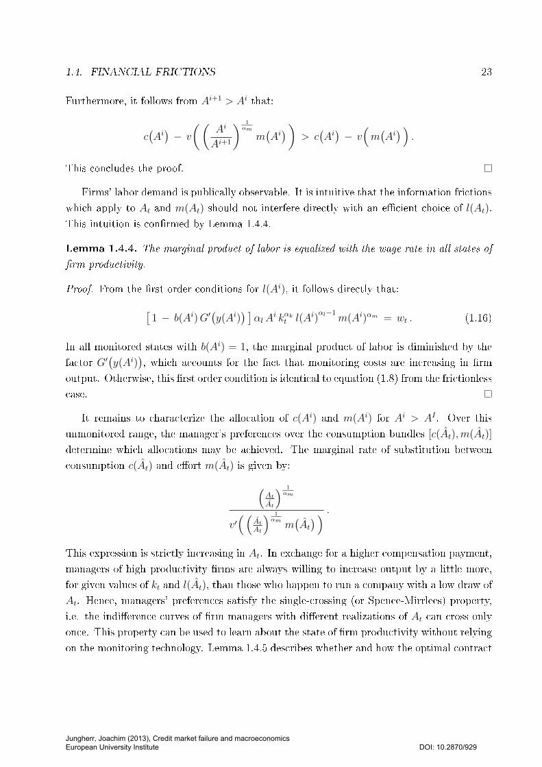
1.4. FINANCIAL FRICTIONS 23
Furthermore, it follows from Ai+1 > Ai that:
c(Ai)− v
((Ai
Ai+1
) 1αm
m(Ai))
> c(Ai)− v
(m(Ai) )
.
This concludes the proof.
Firms' labor demand is publically observable. It is intuitive that the information frictions
which apply to At and m(At) should not interfere directly with an ecient choice of l(At).
This intuition is conrmed by Lemma 1.4.4.
Lemma 1.4.4. The marginal product of labor is equalized with the wage rate in all states of
rm productivity.
Proof. From the rst order conditions for l(Ai), it follows directly that:[1 − b(Ai)G′
(y(Ai)
) ]αlA
i kαkt l(Ai)αl−1
m(Ai)αm = wt . (1.16)
In all monitored states with b(Ai) = 1, the marginal product of labor is diminished by the
factor G′(y(Ai)
), which accounts for the fact that monitoring costs are increasing in rm
output. Otherwise, this rst order condition is identical to equation (1.8) from the frictionless
case.
It remains to characterize the allocation of c(Ai) and m(Ai) for Ai > AI . Over this
unmonitored range, the manager's preferences over the consumption bundles [c(At),m(At)]
determine which allocations may be achieved. The marginal rate of substitution between
consumption c(At) and eort m(At) is given by:
(AtAt
) 1αm
v′((
AtAt
) 1αm
m(At) ) .
This expression is strictly increasing in At. In exchange for a higher compensation payment,
managers of high productivity rms are always willing to increase output by a little more,
for given values of kt and l(At), than those who happen to run a company with a low draw of
At. Hence, managers' preferences satisfy the single-crossing (or Spence-Mirrlees) property,
i.e. the indierence curves of rm managers with dierent realizations of At can cross only
once. This property can be used to learn about the state of rm productivity without relying
on the monitoring technology. Lemma 1.4.5 describes whether and how the optimal contract
Jungherr, Joachim (2013), Credit market failure and macroeconomics European University Institute
DOI: 10.2870/929
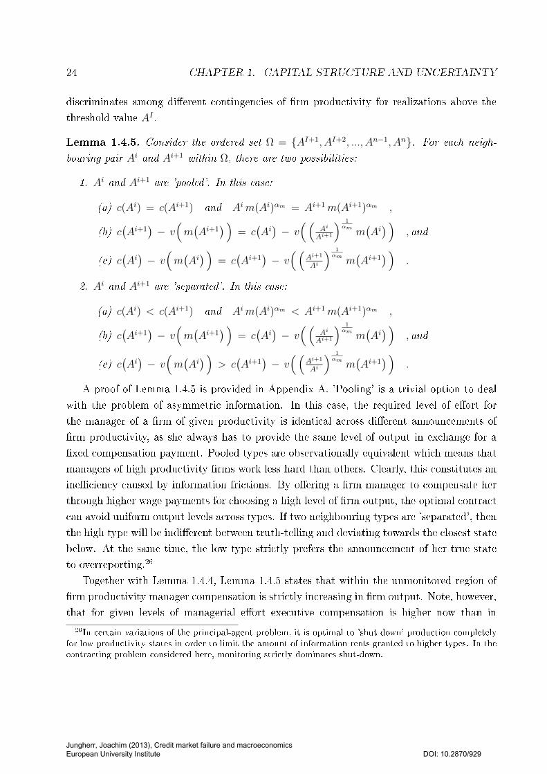
24 CHAPTER 1. CAPITAL STRUCTURE AND UNCERTAINTY
discriminates among dierent contingencies of rm productivity for realizations above the
threshold value AI .
Lemma 1.4.5. Consider the ordered set Ω = AI+1, AI+2, ..., An−1, An. For each neigh-
bouring pair Ai and Ai+1 within Ω, there are two possibilities:
1. Ai and Ai+1 are 'pooled'. In this case:
(a) c(Ai) = c(Ai+1) and Aim(Ai)αm = Ai+1m(Ai+1)αm ,
(b) c(Ai+1
)− v
(m(Ai+1
) )= c
(Ai)− v
((Ai
Ai+1
) 1αm
m(Ai) )
, and
(c) c(Ai)− v
(m(Ai) )
= c(Ai+1
)− v
((Ai+1
Ai
) 1αm
m(Ai+1
) ).
2. Ai and Ai+1 are 'separated'. In this case:
(a) c(Ai) < c(Ai+1) and Aim(Ai)αm < Ai+1 m(Ai+1)αm ,
(b) c(Ai+1
)− v
(m(Ai+1
) )= c
(Ai)− v
((Ai
Ai+1
) 1αm
m(Ai) )
, and
(c) c(Ai)− v
(m(Ai) )
> c(Ai+1
)− v
((Ai+1
Ai
) 1αm
m(Ai+1
) ).
A proof of Lemma 1.4.5 is provided in Appendix A. 'Pooling' is a trivial option to deal
with the problem of asymmetric information. In this case, the required level of eort for
the manager of a rm of given productivity is identical across dierent announcements of
rm productivity, as she always has to provide the same level of output in exchange for a
xed compensation payment. Pooled types are observationally equivalent which means that
managers of high productivity rms work less hard than others. Clearly, this constitutes an
ineciency caused by information frictions. By oering a rm manager to compensate her
through higher wage payments for choosing a high level of rm output, the optimal contract
can avoid uniform output levels across types. If two neighbouring types are 'separated', then
the high type will be indierent between truth-telling and deviating towards the closest state
below. At the same time, the low type strictly prefers the announcement of her true state
to overreporting.26
Together with Lemma 1.4.4, Lemma 1.4.5 states that within the unmonitored region of
rm productivity manager compensation is strictly increasing in rm output. Note, however,
that for given levels of managerial eort executive compensation is higher now than in
26In certain variations of the principal-agent problem, it is optimal to 'shut down' production completelyfor low productivity states in order to limit the amount of information rents granted to higher types. In thecontracting problem considered here, monitoring strictly dominates shut-down.
Jungherr, Joachim (2013), Credit market failure and macroeconomics European University Institute
DOI: 10.2870/929
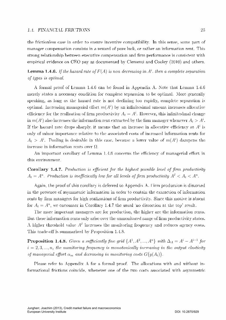
1.4. FINANCIAL FRICTIONS 25
the frictionless case in order to ensure incentive compatibility. In this sense, some part of
manager compensation consists in a reward of pure luck, or rather an information rent. This
strong relationship between executive compensation and rm performance is consistent with
empirical evidence on CEO pay as documented by Clementi and Cooley (2010) and others.
Lemma 1.4.6. If the hazard rate of F (A) is non-decreasing in Ai, then a complete separation
of types is optimal.
A formal proof of Lemma 1.4.6 can be found in Appendix A. Note that Lemma 1.4.6
merely states a necessary condition for complete separation to be optimal. More generally
speaking, as long as the hazard rate is not declining too rapidly, complete separation is
optimal. Increasing managerial eort m(Ai) by an innitesimal amount increases allocative
eciency for the realization of rm productivity At = Ai. However, this innitesimal change
inm(Ai) also increases the information rent extracted by the rm manager whenever At > Ai.
If the hazard rate drops sharply, it means that an increase in allocative eciency at Ai is
only of minor importance relative to the associated costs of increased information rents for
At > Ai. Pooling is desirable in this case, because a lower value of m(Ai) dampens the
increase in information rents over Ω.
An important corollary of Lemma 1.4.6 concerns the eciency of managerial eort in
this environment.
Corollary 1.4.7. Production is ecient for the highest possible level of rm productivity
At = An. Production is ineciently low for all levels of rm productivity AI < At < An.
Again, the proof of this corollary is deferred to Appendix A. Firm production is distorted
in the presence of asymmetric information in order to contain the extraction of information
rents by rm managers for high realizations of rm productivity. Since this motive is absent
for At = An, we encounter in Corollary 1.4.7 the usual `no distortion at the top' result.
The more important managers are for production, the higher are the information rents.
But these information rents only arise over the unmonitored range of rm productivity states.
A higher threshold value AI increases the monitoring frequency and reduces agency costs.
This trade-o is summarized by Proposition 1.4.8.
Proposition 1.4.8. Given a suciently ne grid A1, A2, ..., An with ∆A = Ai −Ai−1 for
i = 2, 3, ..., n, the monitoring frequency is monotonically increasing in the output elasticity
of managerial eort αm and decreasing in monitoring costs G(y(At)
).
Please refer to Appendix A for a formal proof. The allocations with and without in-
formational frictions coincide, whenever one of the two costs associated with asymmetric
Jungherr, Joachim (2013), Credit market failure and macroeconomics European University Institute
DOI: 10.2870/929
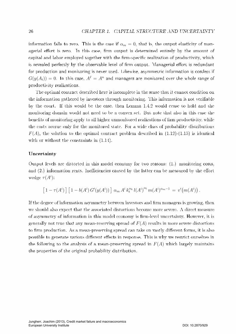
26 CHAPTER 1. CAPITAL STRUCTURE AND UNCERTAINTY
information falls to zero. This is the case if αm = 0, that is, the output elasticity of man-
agerial eort is zero. In this case, rm output is determined entirely by the amount of
capital and labor employed together with the rm-specic realization of productivity, which
is revealed perfectly by the observable level of rm output. Managerial eort is redundant
for production and monitoring is never used. Likewise, asymmetric information is costless if
G(y(At)) = 0. In this case, AI = An and managers are monitored over the whole range of
productivity realizations.
The optimal contract described here is incomplete in the sense that it cannot condition on
the information gathered by investors through monitoring. This information is not veriable
by the court. If this would be the case, then Lemma 1.4.2 would cease to hold and the
monitoring domain would not need to be a convex set. But note that also in this case the
benets of monitoring apply to all higher unmonitored realizations of rm productivity, while
the costs accrue only for the monitored state. For a wide class of probability distributions
F (A), the solution to the optimal contract problem described in (1.12)-(1.15) is identical
with or without the constraints in (1.14).
Uncertainty
Output levels are distorted in this model economy for two reasons: (1.) monitoring costs,
and (2.) information rents. Ineciencies caused by the latter can be measured by the eort
wedge τ(Ai):[1− τ(Ai)
] [1− b(Ai)G′(y(Ai))
]αmA
i kαkt l(Ai)αlm(Ai)αm−1 = v′
(m(Ai)
).
If the degree of information asymmetry between investors and rm managers is growing, then
we should also expect that the associated distortions become more severe. A direct measure
of asymmetry of information in this model economy is rm-level uncertainty. However, it is
generally not true that any mean-reserving spread of F (A) results in more severe distortions
to rm production. As a mean-preserving spread can take on vastly dierent forms, it is also
possible to generate various dierent eects in response. This is why we restrict ourselves in
the following to the analysis of a mean-preserving spread in F (A) which largely maintains
the properties of the original probability distribution.
Jungherr, Joachim (2013), Credit market failure and macroeconomics European University Institute
DOI: 10.2870/929
1.4. FINANCIAL FRICTIONS 27
Proposition 1.4.9. Consider the range of all possible productivity levels A1, A2, ..., Anwith ∆A = Ai − Ai−1 for i = 2, 3, ..., n. Furthermore, consider an increase in ∆A which
leaves all probabilities p(Ai) and the expected value of At unchanged. If this spread is of
sucient size, then monitoring is optimally used more frequently in the new contract and the
value of τ(Ai) has to increase for each Ai.
Proof. First of all, note that information rents are increasing in ∆A. Consequently, man-
agerial eort levels for AI+1 < At < An are falling in response to an increase in ∆A as can
be seen from equation (1.21). The associated values of τ(Ai) are growing. This increase in
information rents shifts the trade-o which determines the optimal threshold value AI as de-
scribed in Proposition 1.4.8. The labor wedge τ(AI+1) is growing towards one in ∆A, which
implies that the benets of increasing the monitoring range are growing without bounds.
Recall that rm technology satises the Inada conditions. At some point, the benets of
an additional increase in AI must outweigh the associated costs. The discrete support of
rm productivity allows for a local drop in the value of τ(Ai) for some Ai in response to an
increase in AI . However, if ∆A continues to grow, both the monitoring frequency as well as
the eort wedge for all unmonitored realizations (except for An) need to increase.
Now that we have characterized the solution to the contracting problem given in (1.12)-
(1.15), and understood the role of agency costs, monitoring costs, and rm-level uncertainty
in shaping the production outcomes in this model economy, we go on to examine the implica-
tions of these results for the behavior of capital structure, default rates, and rm productivity
over the business cycle.
1.4.2 Capital Structure
The previous section examined the problem of a manager who has to decide about the
optimal contract to oer on the period t− 1 capital market in the presence of informational
frictions. Key components of this contract are the optimal monitoring frequency and an
executive compensation scheme which incentivizes the rm manager to exert high eort
levels even in the presence of asymmetric information. In principle, this contract could be
implemented using various types of nancial securities as long as they result in the solution
to the contracting problem described above. It turns out, however, that one implementation
of the optimal contract consists of a certain combination of public equity and corporate
bonds. This implementation of the optimal contract corresponds closely to the practice of
rm nancing of publicly held companies and is therefore particularly attractive in order to
Jungherr, Joachim (2013), Credit market failure and macroeconomics European University Institute
DOI: 10.2870/929
28 CHAPTER 1. CAPITAL STRUCTURE AND UNCERTAINTY
understand the eects of changes in fundamentals on the nancing choice and the economic
performance of publicly held rms. Equity and bond securities are dened as follows.
Denition Equity holders are the residual claimants of a rm. They are entitled to a pro
rata share of the rm's asset value net of wage, manager compensation, and debt payments.
Denition Bond holders are entitled to a xed payment by the debtor at maturity. In case
the debtor fails to comply with this obligation, bankruptcy is declared and bond holders
have the right to recover as much of the face value of their bonds as possible.
One way to characterize the key dierence between these two nancing instruments is:
Equity is soft; debt is hard. A bond represents a precisely dened claim which is senior
to equity and highly enforceable with the occasional upshot of bankruptcy of the debtor.
Meanwhile, equity generates a highly variable future payo which is junior to debt and wage
obligations.
We follow Townsend (1979) and Gale and Hellwig (1985) in identifying bankruptcy with
monitoring. The social value of bankruptcy proceedings consists of a costly transfer of rm-
specic information to outsiders, i.e. creditors. This view on bankruptcy and rm default
allows us to separate the state-dependent payout to investors implied by the optimal contract
into distinct payments to holders of equity securities and bonds, respectively. Whenever a
rm fails to pay out the face value of debt:
y(AI+1) + (1− δ) kt − wt l(AI+1) − c(AI+1)
to bond holders, the rm goes bankrupt and monitoring takes place. This allows for recon-
tracting between the bond holders (or their representatives) and the rm manager without
the complications of asymmetric information. However, putting the rm under the scrutiny
of creditors comes at a cost as accountants and lawyers need to be paid during the process of
bankruptcy. This implies for the aggregate payout to the bond holders of a given company:
P d(At) =
y(AI+1) + (1− δ) kt − wt l(AI+1) − c(AI+1) , if At > AI , and
y(At) − G(y(At)
)+ (1− δ) kt − wt l(At) − c(At) , otherwise.
Whenever the ex-post value of a rm is high enough to pay out bond holders, they receive
a xed payment equal to the face value of their debt holdings. In case the rm is unable to
service these obligations, bankruptcy is declared, monitoring takes place, and the creditors
receive whatever is left of the company. Within this bankruptcy region, the xed debt claim
Jungherr, Joachim (2013), Credit market failure and macroeconomics European University Institute
DOI: 10.2870/929
1.4. FINANCIAL FRICTIONS 29
becomes state-dependent. Holders of equity securities receive the residual asset value after
all liabilities have been served. This results in an aggregate payout to holders of equity
securities issued by a given company as given by:
P e(At) =
y(At)− y(AI+1)− wt[l(At)− l(AI+1)
]−[c(At)− c(AI+1)
], if At > AI ,
0 , otherwise.
Dividends are state-dependent and only paid out as long as the rm is able to service its debt
and wage obligations. A look at Propositions 1.4.8 and 1.4.9 through the lens of nancial
structure links bankruptcy risk to characteristics of the economic environment. Bankruptcy
is used in order to contain agency costs. As these costs increase (1.) in the degree of
asymmetry of information between investors and managers and (2.) in the importance of
managers for production outcomes, bankruptcy is used more frequently in response to an
increase in one of these two factors. Obviously, the opposite is true for a rise in bankruptcy
costs. The positive relationship between rm-specic uncertainty and bankruptcy risk nds
empirical support in Gilchrist, Sim, and Zakraj²ek (2010), who estimate a positive eect of
uncertainty on corporate bond spreads.
Note that so far we have only separated the rm payout to investors into distinct payments
to equity and bond holders. It remains to relate these ndings to the optimal capital structure
choice of the rm. This can only be done in general equilibrium as is shown below. We denote
the household's holdings of debt and equity securities issued by rm j at the end of period t−1
with dt(j) and et(j), respectively. The gross return realized on these nancial investments
is given by Rdt (j) and Re
t (j). Our denition of a competitive equilibrium is adapted to the
introduction of nancial structure in the following way.
Denition For all histories of aggregate shocks to Ft+i+1(A) and given some initial wealth
level Wt, a competitive equilibrium in this economy consists of prices w∗t+i+1, Rd∗t+i+1(j),
Re∗t+i+1(j), and quantities Ct+i, lt+i+1, d
∗t+i+1(j), and e∗t+i+1(j), such that (1.) households
solve their individual optimization problem, and (2.) labor and capital markets clear.
Jungherr, Joachim (2013), Credit market failure and macroeconomics European University Institute
DOI: 10.2870/929
30 CHAPTER 1. CAPITAL STRUCTURE AND UNCERTAINTY
1.4.3 Households
Revisiting the representative household's problem, we examine its portfolio choice among
the various equity and debt securities oered by dierent managers on the capital market:
maxCt+i,dt+i+1(j),
et+i+1(j),lt+i∈R≥0
Et∞∑i=0
βi[U(Ct+i) − V (lt+i)
](1.17)
subject to: Ct+i +
∫ 1
0
[dt+i+1(j) + et+i+1(j)
]dj
≤ wt+i lt+i +
∫ 1
0
[Rdt+i(j) dt+i(j) + Re
t+i(j) et+i(j)]dj . (1.18)
The rst-order condition with respect to labor supply is identical to the frictionless case:
V ′(lht ) = wt U′(Ch
t ) . (1.19)
Savings are chosen in order to equalize the expected marginal utility from adjusting the
portfolio weight of any type of security which is in positive demand:
U ′(Cht ) = β Et
[U ′(Ch
t+1)Rit+1(j)
], for i = d, e, and for all j . (1.20)
Just as in the frictionless case discussed above, the optimal portfolio of risk-averse households
is perfectly diversied across rms which are all subject to idiosyncratic risk and identical
ex-ante. Since the portfolio weight of any given security of any given rm is zero, households
are perfectly insured against rm-specic risks. Furthermore, households already know at
time t next period's distribution of productivity shocks Ft+1(A). For this reason, they do
not face aggregate uncertainty in their savings decision and only care about the expected
return associated with the various securities oered on the capital market.
Jungherr, Joachim (2013), Credit market failure and macroeconomics European University Institute
DOI: 10.2870/929
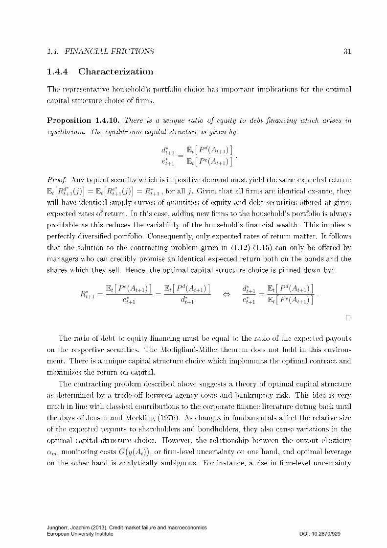
1.4. FINANCIAL FRICTIONS 31
1.4.4 Characterization
The representative household's portfolio choice has important implications for the optimal
capital structure choice of rms.
Proposition 1.4.10. There is a unique ratio of equity to debt nancing which arises in
equilibrium. The equilibrium capital structure is given by:
d∗t+1
e∗t+1
=Et[P d(At+1)
]Et[P e(At+1)
] .Proof. Any type of security which is in positive demand must yield the same expected return:
Et[Rd∗t+1(j)
]= Et
[Re∗t+1(j)
]= R∗t+1 , for all j. Given that all rms are identical ex-ante, they
will have identical supply curves of quantities of equity and debt securities oered at given
expected rates of return. In this case, adding new rms to the household's portfolio is always
protable as this reduces the variability of the household's nancial wealth. This implies a
perfectly diversied portfolio. Consequently, only expected rates of return matter. It follows
that the solution to the contracting problem given in (1.12)-(1.15) can only be oered by
managers who can credibly promise an identical expected return both on the bonds and the
shares which they sell. Hence, the optimal capital structure choice is pinned down by:
R∗t+1 =Et[P e(At+1)
]e∗t+1
=Et[P d(At+1)
]d∗t+1
⇔d∗t+1
e∗t+1
=Et[P d(At+1)
]Et[P e(At+1)
] .
The ratio of debt to equity nancing must be equal to the ratio of the expected payouts
on the respective securities. The Modigliani-Miller theorem does not hold in this environ-
ment. There is a unique capital structure choice which implements the optimal contract and
maximizes the return on capital.
The contracting problem described above suggests a theory of optimal capital structure
as determined by a trade-o between agency costs and bankruptcy risk. This idea is very
much in line with classical contributions to the corporate nance literature dating back until
the days of Jensen and Meckling (1976). As changes in fundamentals aect the relative size
of the expected payouts to shareholders and bondholders, they also cause variations in the
optimal capital structure choice. However, the relationship between the output elasticity
αm, monitoring costs G(y(At)
), or rm-level uncertainty on one hand, and optimal leverage
on the other hand is analytically ambiguous. For instance, a rise in rm-level uncertainty
Jungherr, Joachim (2013), Credit market failure and macroeconomics European University Institute
DOI: 10.2870/929
32 CHAPTER 1. CAPITAL STRUCTURE AND UNCERTAINTY
increases the risk of bankruptcy, but the associated change in the optimal face value of
debt may be positive or negative. And even if the face value of debt is higher now, the
rm is more unlikely to actually meet its credit obligations. If bondholders gain relative to
shareholders, then the optimal ratio of debt to equity nancing must increase and vice versa.
The comparative statics of optimal capital structure generally depend on the functional
form of the probability distribution F (A), the monitoring costs G(y(At)
), as well as other
parameters.
The theoretical predictions are more clear cut when it comes to examine the impact of
a rise in rm-level uncertainty on the distortions to rm production. From Lemma 1.4.9
we know that both the eort wedge and the risk of bankruptcy are increasing in uncer-
tainty. Firm output is therefore falling relative to its perfect information benchmark. This
counteracts the procyclical role of uncertainty in the frictionsless benchmark economy (see
Proposition 1.3.3). Whether the `Oi-Hartman-Abel' eect or the increase in the costs of
asymmetric information prevail in response to a rise in rm-level uncertainty is a question
which requires a quantitative answer.
1.5 Quantitative Analysis
In order to get a more precise idea about the role of idiosyncratic uncertainty in shaping
the behavior of corporate capital structure and rm production along the business cycle, the
theoretical model economy is parameterized using U.S. data and its properties are studied
in response to rm-level uncertainty shocks. I choose the following functional forms:
• Firm managers' disutility of eort is linear: v(mt(j)
)= γ mt(j) .
• Households' disutility of work is zero: V (lt) = 0 .
It follows that in equilibrium households always supply their entire endowment of working
time l = 1. Working hours are constant over the business cycle and only the competitive
wage rate moves with aggregate conditions. One dierence between this simulated economy
and the analytical model outlined above concerns the timing.
• Firm managers hire labor before the realization of the rm-specic productivity shock
At(j).
This implies that all rms hire an identical amount of labor.
Jungherr, Joachim (2013), Credit market failure and macroeconomics European University Institute
DOI: 10.2870/929
1.5. QUANTITATIVE ANALYSIS 33
1.5.1 Parametrization
The period in the model is a quarter. Most of the parameters can be calibrated using
long term averages of stationary target variables. The stochastic process of time-varying
uncertainty is specied in order to replicate empirical evidence provided by Bloom et al.
(2012) on the properties of the cross-sectional distribution of rm-specic productivity shocks
over time.
Parameters with long run average targets
We have seen above that two of the key determinants of capital structure in this model are
the output elasticity of managerial eort αm and bankruptcy costs G(yt). We set αm = 0.05,
which results in a high share of average executive compensation in rm earnings. Bebchuk
and Grinstein (2005) estimate the compensation of the top ve executives of each rms in
their sample of public companies to add up to 6.6% of rm earnings. Arguably, the group
of managers which are subject to the agency problem described above can be much bigger
than only the top ve managers of a given rm. On the other hand, the assumed production
function suggests that these managers should be able to inuence with their actions the
aggregate production outcome of the entire company. The chosen parameter value is a
preliminary choice and subject to future adjustment.
Bankruptcy costs are assumed to be proportional to rm output: G(yt) = ϕyt. This
assumption is motivated by the empirical ndings of Bris, Welch and Zhu (2006). The
authors document the amount of fees paid to attorneys, accountants and trustees during
bankruptcy proceedings to be increasing in rm size.27 The parameter ϕ is set to 0.24,
which implies average bankruptcy costs of 13.65% of rm asset value. This lies well within
the range of empirical estimates.28 The model generates yearly default rates of 2.65%, which
is slightly higher than the default rate on corporate bonds of 2.20% reported in Covas and
Den Haan (2011).
Covas and Den Haan (2011) and Jermann and Quadrini (2012) calculate average leverage
of publicly traded rms as the ratio of liabilities to the book value of rm assets. They report
values of 0.59 and 0.46, respectively. In order to simultaneously match empirical default rates
and the fairly low ratio of debt nancing in the data, a high value of capital depreciation is
27Meisenzahl (2011) reports that the assumption of proportional monitoring costs ts the data on USsmall business credit contracts quite well. Other models which assume proportional monitoring costs includeCarlstrom and Fuerst (1997), Bernanke, Gertler and Gilchrist (1999), and Christiano, Motto and Rostagno(2013).
28Bris, Welch, and Zhu (2006) report an estimate of 10% with a broad range of tted values from 0% to20% depending on rm characteristics.
Jungherr, Joachim (2013), Credit market failure and macroeconomics European University Institute
DOI: 10.2870/929
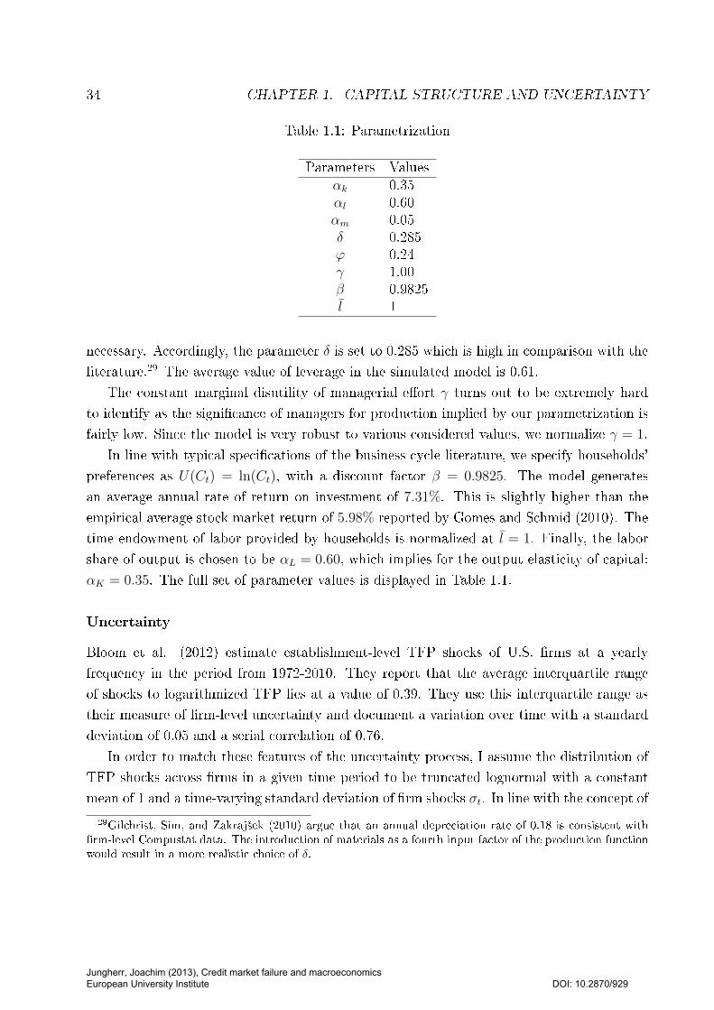
34 CHAPTER 1. CAPITAL STRUCTURE AND UNCERTAINTY
Table 1.1: Parametrization
Parameters Valuesαk 0.35αl 0.60αm 0.05δ 0.285ϕ 0.24γ 1.00β 0.9825l 1
necessary. Accordingly, the parameter δ is set to 0.285 which is high in comparison with the
literature.29 The average value of leverage in the simulated model is 0.61.
The constant marginal disutility of managerial eort γ turns out to be extremely hard
to identify as the signicance of managers for production implied by our parametrization is
fairly low. Since the model is very robust to various considered values, we normalize γ = 1.
In line with typical specications of the business cycle literature, we specify households'
preferences as U(Ct) = ln(Ct), with a discount factor β = 0.9825. The model generates
an average annual rate of return on investment of 7.31%. This is slightly higher than the
empirical average stock market return of 5.98% reported by Gomes and Schmid (2010). The
time endowment of labor provided by households is normalized at l = 1. Finally, the labor
share of output is chosen to be αL = 0.60, which implies for the output elasticity of capital:
αK = 0.35. The full set of parameter values is displayed in Table 1.1.
Uncertainty
Bloom et al. (2012) estimate establishment-level TFP shocks of U.S. rms at a yearly
frequency in the period from 1972-2010. They report that the average interquartile range
of shocks to logarithmized TFP lies at a value of 0.39. They use this interquartile range as
their measure of rm-level uncertainty and document a variation over time with a standard
deviation of 0.05 and a serial correlation of 0.76.
In order to match these features of the uncertainty process, I assume the distribution of
TFP shocks across rms in a given time period to be truncated lognormal with a constant
mean of 1 and a time-varying standard deviation of rm shocks σt. In line with the concept of
29Gilchrist, Sim, and Zakraj²ek (2010) argue that an annual depreciation rate of 0.18 is consistent withrm-level Compustat data. The introduction of materials as a fourth input factor of the production functionwould result in a more realistic choice of δ.
Jungherr, Joachim (2013), Credit market failure and macroeconomics European University Institute
DOI: 10.2870/929
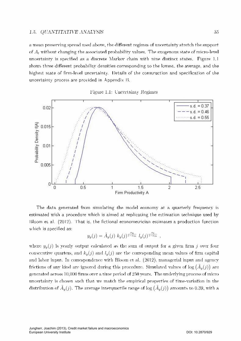
1.5. QUANTITATIVE ANALYSIS 35
a mean preserving spread used above, the dierent regimes of uncertainty stretch the support
of At without changing the associated probability values. The exogenous state of micro-level
uncertainty is specied as a discrete Markov chain with nine distinct states. Figure 1.1
shows three dierent probability densities corresponding to the lowest, the average, and the
highest state of rm-level uncertainty. Details of the construction and specication of the
uncertainty process are provided in Appendix B.
Figure 1.1: Uncertainty Regimes
The data generated from simulating the model economy at a quarterly frequency is
estimated with a procedure which is aimed at replicating the estimation technique used by
Bloom et al. (2012). That is, the ctional econometrician estimates a production function
which is specied as:
yy(j) = Ay(j) ky(j)αk
1−αm ly(j)αl
1−αm ,
where yy(j) is yearly output calculated as the sum of output for a given rm j over four
consecutive quarters, and ky(j) and ly(j) are the corresponding mean values of rm capital
and labor input. In correspondence with Bloom et al. (2012), managerial input and agency
frictions of any kind are ignored during this procedure. Simulated values of log(Ay(j)
)are
generated across 10,000 rms over a time period of 250 years. The underlying process of micro
uncertainty is chosen such that we match the empirical properties of time-variation in the
distribution of Ay(j). The average interquartile range of log(Ay(j)
)amounts to 0.39, with a
Jungherr, Joachim (2013), Credit market failure and macroeconomics European University Institute
DOI: 10.2870/929
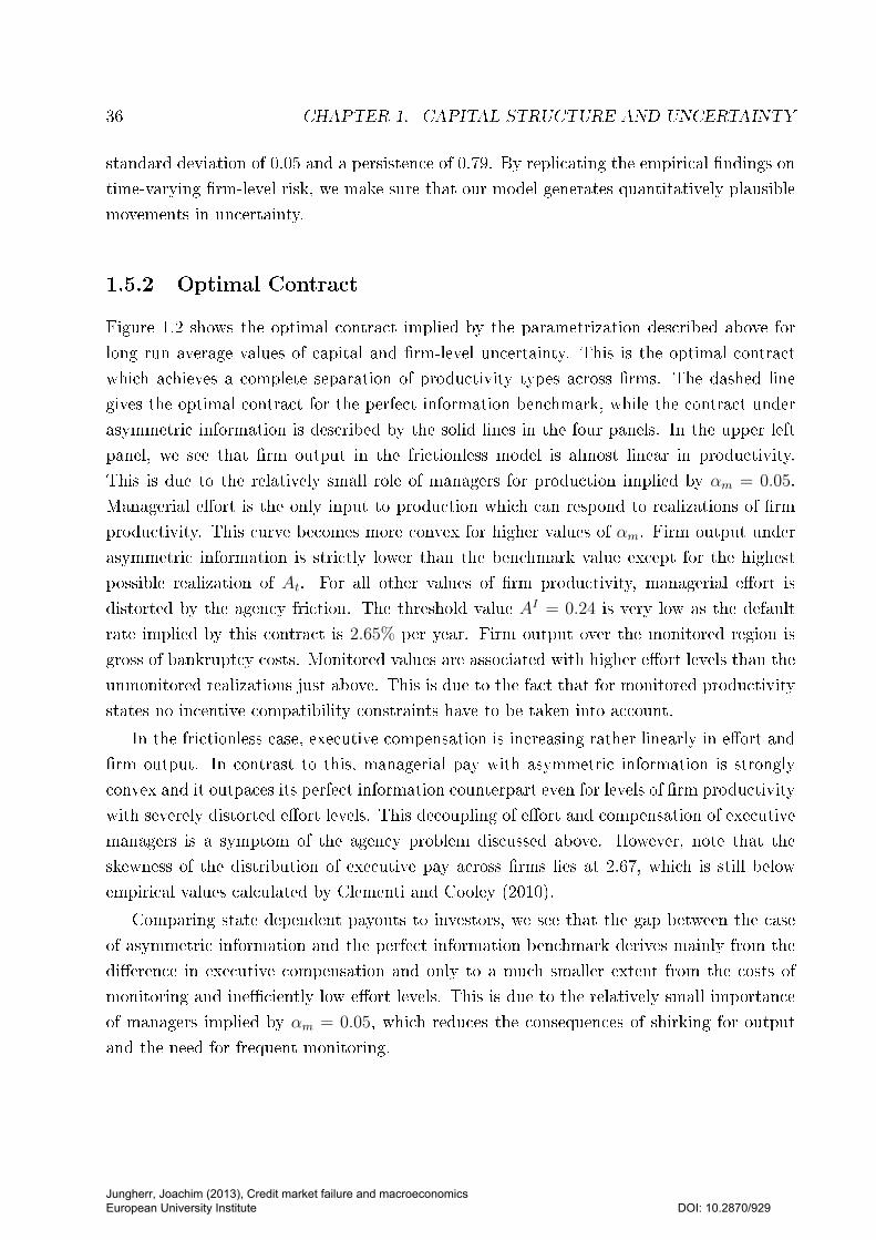
36 CHAPTER 1. CAPITAL STRUCTURE AND UNCERTAINTY
standard deviation of 0.05 and a persistence of 0.79. By replicating the empirical ndings on
time-varying rm-level risk, we make sure that our model generates quantitatively plausible
movements in uncertainty.
1.5.2 Optimal Contract
Figure 1.2 shows the optimal contract implied by the parametrization described above for
long run average values of capital and rm-level uncertainty. This is the optimal contract
which achieves a complete separation of productivity types across rms. The dashed line
gives the optimal contract for the perfect information benchmark, while the contract under
asymmetric information is described by the solid lines in the four panels. In the upper left
panel, we see that rm output in the frictionless model is almost linear in productivity.
This is due to the relatively small role of managers for production implied by αm = 0.05.
Managerial eort is the only input to production which can respond to realizations of rm
productivity. This curve becomes more convex for higher values of αm. Firm output under
asymmetric information is strictly lower than the benchmark value except for the highest
possible realization of At. For all other values of rm productivity, managerial eort is
distorted by the agency friction. The threshold value AI = 0.24 is very low as the default
rate implied by this contract is 2.65% per year. Firm output over the monitored region is
gross of bankruptcy costs. Monitored values are associated with higher eort levels than the
unmonitored realizations just above. This is due to the fact that for monitored productivity
states no incentive compatibility constraints have to be taken into account.
In the frictionless case, executive compensation is increasing rather linearly in eort and
rm output. In contrast to this, managerial pay with asymmetric information is strongly
convex and it outpaces its perfect information counterpart even for levels of rm productivity
with severely distorted eort levels. This decoupling of eort and compensation of executive
managers is a symptom of the agency problem discussed above. However, note that the
skewness of the distribution of executive pay across rms lies at 2.67, which is still below
empirical values calculated by Clementi and Cooley (2010).
Comparing state dependent payouts to investors, we see that the gap between the case
of asymmetric information and the perfect information benchmark derives mainly from the
dierence in executive compensation and only to a much smaller extent from the costs of
monitoring and ineciently low eort levels. This is due to the relatively small importance
of managers implied by αm = 0.05, which reduces the consequences of shirking for output
and the need for frequent monitoring.
Jungherr, Joachim (2013), Credit market failure and macroeconomics European University Institute
DOI: 10.2870/929
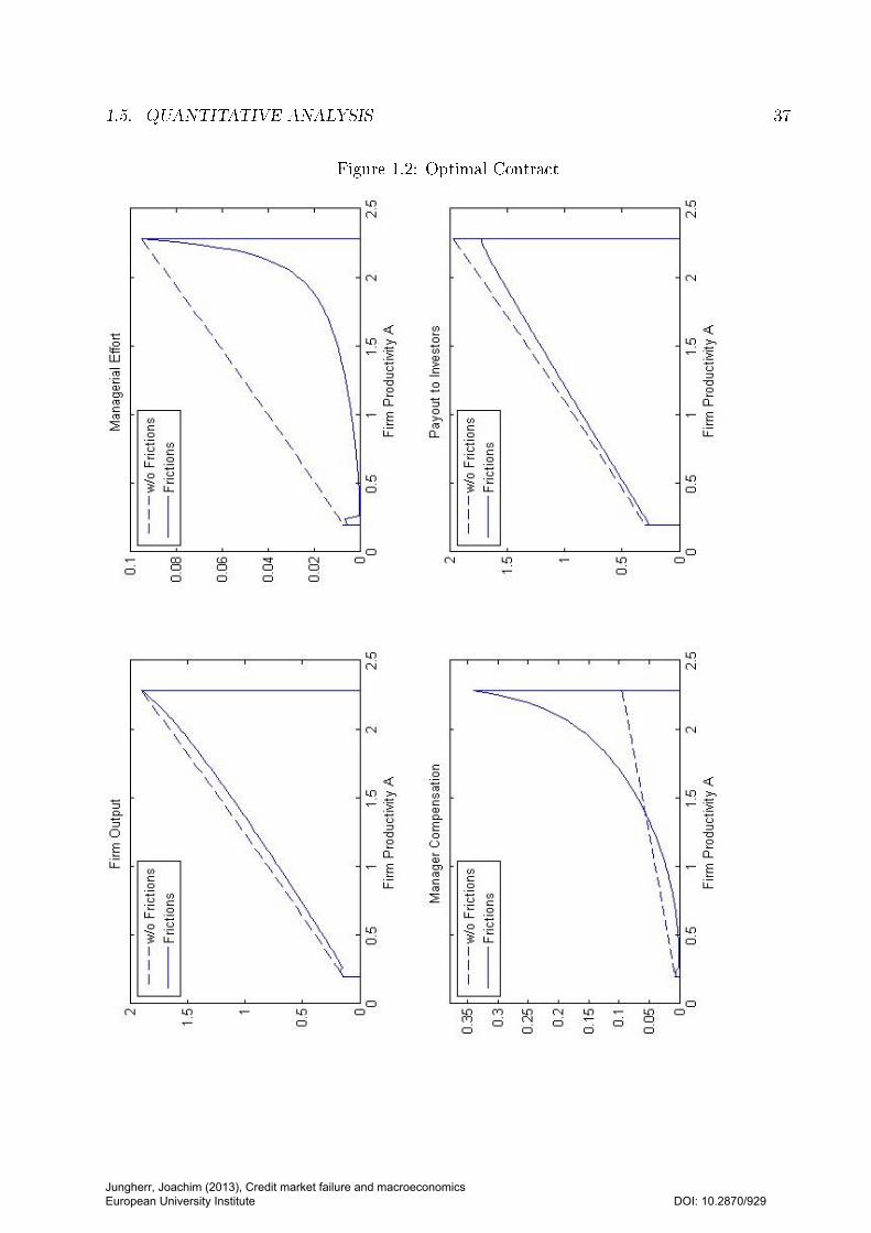
1.5. QUANTITATIVE ANALYSIS 37
Figure 1.2: Optimal Contract
Jungherr, Joachim (2013), Credit market failure and macroeconomics European University Institute
DOI: 10.2870/929
38 CHAPTER 1. CAPITAL STRUCTURE AND UNCERTAINTY
Figure 1.3: Uncertainty and Expected Returns
1.5.3 Uncertainty and Financial Markets
Figure 1.3 shows the two competing forces which move the return on investment for diering
degrees of rm-level risk. Consider rst the case of perfect information in the upper panel.
In the version of the model used for the numerical analysis, labor demand does not respond
to the rm-specic realization of productivity and the disutility of managerial eort is linear.
In this case, ecient eort levels are strictly convex in At(j). Consequently, also rm output
and the payouts to investors are convex in rm productivity. The `Oi-Hartman-Abel' eect
gives rise to the familiar procyclical behavior of rm-level risk.
In the lower panel of Figure 1.3, the expected return to investment is displayed for
the case of information frictions. The benecial impact of rising uncertainty present in
the frictionless environment is still at work here. But in addition to this, uncertainty also
drives up monitoring and agency costs which depresses investors' returns. It turns out that
uncertainty's impact on the costs of asymmetric information is getting weaker for higher
levels of rm risk. This results in a non-monotonic relationship between the expected return
to investment and rm-level uncertainty. What is the eect of rising uncertainty on the
optimal nancing mix of publicly traded rms? Figure 1.4 shows the aggregate payout
to shareholders and bondholders given the long-run average capital stock for the dierent
uncertainty regimes. The expected value of total payouts to debt holders is monotonically
decreasing in uncertainty. This negative eect of volatility on the value of debt claims
Jungherr, Joachim (2013), Credit market failure and macroeconomics European University Institute
DOI: 10.2870/929
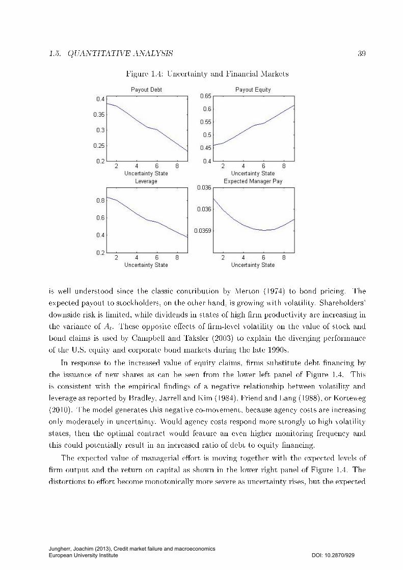
1.5. QUANTITATIVE ANALYSIS 39
Figure 1.4: Uncertainty and Financial Markets
is well understood since the classic contribution by Merton (1974) to bond pricing. The
expected payout to stockholders, on the other hand, is growing with volatility. Shareholders'
downside risk is limited, while dividends in states of high rm productivity are increasing in
the variance of At. These opposite eects of rm-level volatility on the value of stock and
bond claims is used by Campbell and Taksler (2003) to explain the diverging performance
of the U.S. equity and corporate bond markets during the late 1990s.
In response to the increased value of equity claims, rms substitute debt nancing by
the issuance of new shares as can be seen from the lower left panel of Figure 1.4. This
is consistent with the empirical ndings of a negative relationship between volatility and
leverage as reported by Bradley, Jarrell and Kim (1984), Friend and Lang (1988), or Korteweg
(2010). The model generates this negative co-movement, because agency costs are increasing
only moderately in uncertainty. Would agency costs respond more strongly to high volatility
states, then the optimal contract would feature an even higher monitoring frequency and
this could potentially result in an increased ratio of debt to equity nancing.
The expected value of managerial eort is moving together with the expected levels of
rm output and the return on capital as shown in the lower right panel of Figure 1.4. The
distortions to eort become monotonically more severe as uncertainty rises, but the expected
Jungherr, Joachim (2013), Credit market failure and macroeconomics European University Institute
DOI: 10.2870/929
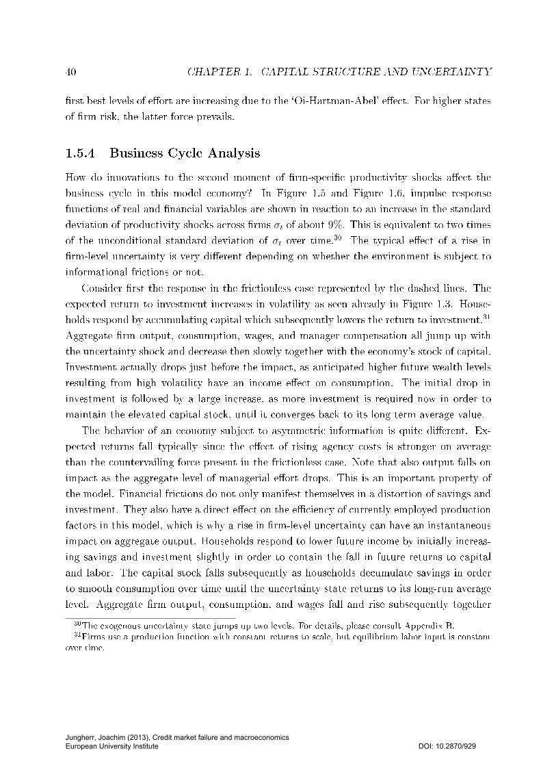
40 CHAPTER 1. CAPITAL STRUCTURE AND UNCERTAINTY
rst best levels of eort are increasing due to the `Oi-Hartman-Abel' eect. For higher states
of rm risk, the latter force prevails.
1.5.4 Business Cycle Analysis
How do innovations to the second moment of rm-specic productivity shocks aect the
business cycle in this model economy? In Figure 1.5 and Figure 1.6, impulse response
functions of real and nancial variables are shown in reaction to an increase in the standard
deviation of productivity shocks across rms σt of about 9%. This is equivalent to two times
of the unconditional standard deviation of σt over time.30 The typical eect of a rise in
rm-level uncertainty is very dierent depending on whether the environment is subject to
informational frictions or not.
Consider rst the response in the frictionless case represented by the dashed lines. The
expected return to investment increases in volatility as seen already in Figure 1.3. House-
holds respond by accumulating capital which subsequently lowers the return to investment.31
Aggregate rm output, consumption, wages, and manager compensation all jump up with
the uncertainty shock and decrease then slowly together with the economy's stock of capital.
Investment actually drops just before the impact, as anticipated higher future wealth levels
resulting from high volatility have an income eect on consumption. The initial drop in
investment is followed by a large increase, as more investment is required now in order to
maintain the elevated capital stock, until it converges back to its long term average value.
The behavior of an economy subject to asymmetric information is quite dierent. Ex-
pected returns fall typically since the eect of rising agency costs is stronger on average
than the countervailing force present in the frictionless case. Note that also output falls on
impact as the aggregate level of managerial eort drops. This is an important property of
the model. Financial frictions do not only manifest themselves in a distortion of savings and
investment. They also have a direct eect on the eciency of currently employed production
factors in this model, which is why a rise in rm-level uncertainty can have an instantaneous
impact on aggregate output. Households respond to lower future income by initially increas-
ing savings and investment slightly in order to contain the fall in future returns to capital
and labor. The capital stock falls subsequently as households decumulate savings in order
to smooth consumption over time until the uncertainty state returns to its long-run average
level. Aggregate rm output, consumption, and wages fall and rise subsequently together
30The exogenous uncertainty state jumps up two levels. For details, please consult Appendix B.31Firms use a production function with constant returns to scale, but equilibrium labor input is constant
over time.
Jungherr, Joachim (2013), Credit market failure and macroeconomics European University Institute
DOI: 10.2870/929

1.5. QUANTITATIVE ANALYSIS 41
with aggregate capital. Also executive compensation is diminished, because managerial ef-
fort is lowered as a result both of the increase in uncertainty and of the lowered stock of rm
capital.
While the responses of real variables (aggregate output, consumption, investment) are
only of limited magnitude in this specication, nancial variables react quite strongly. The
increase in the default rate of 20% depresses the value of debt claims, which leads to a fall of
the absolute amount of debt nancing by 12%. The increase in the value of equity by more
than 6% does not fully make up for the loss in total capital. Leverage decreases by about
18%.
Table 1.2: Business Cycle Properties
Correlation with Output Data Frictions w/o FrictionsFirm-level Uncertainty -0.46 -0.70 0.97Consumption 0.83 0.98 0.99Investment 0.87 0.94 0.96Executive Pay 0.92 0.99 1.00Default Rate -0.33 -0.70
Notes: All variables are logged and measured as deviations from trend. Firm-level Uncertainty is the
cross-sectional interquartile range of establishment-level shocks to logarithmized TFP. The contemporaneous
correlation with GDP is reported by Bloom et al. (2012). The values for Consumption and Investment can
be found in Jermann and Quadrini (2012). The correlation for Executive Pay is provided by Eisfeldt and
Rampini (2008) based on data by Bebchuk and Grinstein (2005). The correlation of output with default
rates is calculated by Gomes and Schmid (2010).
These observations are conrmed by unconditional correlations between aggregate output
and selected variables as generated by simulations of the model with and without asymmetric
information. Table 1.2 compares this simulated data with stylized facts of the business
cycle. In contrast to the frictionless benchmark case, the model with informational frictions
performs well in replicating the countercyclical behavior of rm-level uncertainty and the
default rate on corporate bonds. Consumption, investment, and executive pay are all highly
correlated with aggregate output, both in the data and in the model. Figure 1.7 illustrates
how the results above relate to the empirical importance of time-varying TFP in shaping the
business cycle. The plot shows three simulated time series generated by the model economy
subject to asymmetric information. The rst panel shows logged values of σt, the standard
deviation of productivity shocks across rms, as deviations from the long-run average. The
corresponding reaction of aggregate rm output is displayed below. Times of high volatility
alternate with periods of low variation in output. Whenever rm-level uncertainty is already
Jungherr, Joachim (2013), Credit market failure and macroeconomics European University Institute
DOI: 10.2870/929
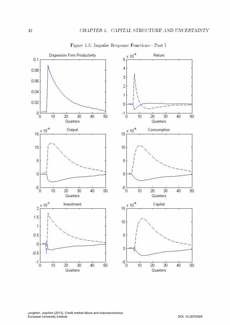
42 CHAPTER 1. CAPITAL STRUCTURE AND UNCERTAINTY
Figure 1.5: Impulse Response Functions - Part I
Jungherr, Joachim (2013), Credit market failure and macroeconomics European University Institute
DOI: 10.2870/929
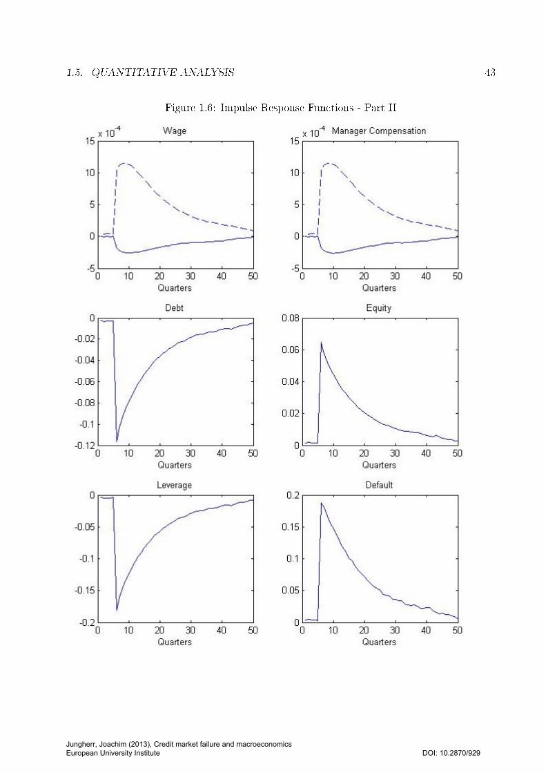
1.5. QUANTITATIVE ANALYSIS 43
Figure 1.6: Impulse Response Functions - Part II
Jungherr, Joachim (2013), Credit market failure and macroeconomics European University Institute
DOI: 10.2870/929
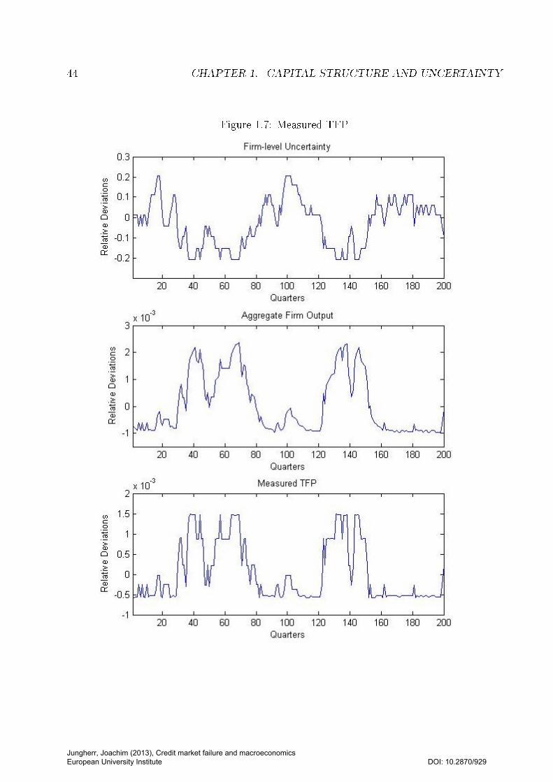
44 CHAPTER 1. CAPITAL STRUCTURE AND UNCERTAINTY
Figure 1.7: Measured TFP
Jungherr, Joachim (2013), Credit market failure and macroeconomics European University Institute
DOI: 10.2870/929
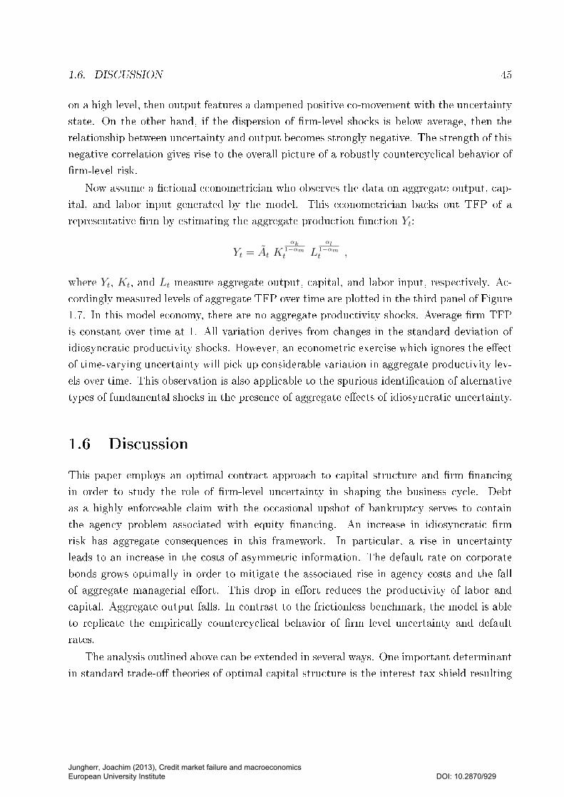
1.6. DISCUSSION 45
on a high level, then output features a dampened positive co-movement with the uncertainty
state. On the other hand, if the dispersion of rm-level shocks is below average, then the
relationship between uncertainty and output becomes strongly negative. The strength of this
negative correlation gives rise to the overall picture of a robustly countercyclical behavior of
rm-level risk.
Now assume a ctional econometrician who observes the data on aggregate output, cap-
ital, and labor input generated by the model. This econometrician backs out TFP of a
representative rm by estimating the aggregate production function Yt:
Yt = At Kαk
1−αmt L
αl1−αmt ,
where Yt, Kt, and Lt measure aggregate output, capital, and labor input, respectively. Ac-
cordingly measured levels of aggregate TFP over time are plotted in the third panel of Figure
1.7. In this model economy, there are no aggregate productivity shocks. Average rm TFP
is constant over time at 1. All variation derives from changes in the standard deviation of
idiosyncratic productivity shocks. However, an econometric exercise which ignores the eect
of time-varying uncertainty will pick up considerable variation in aggregate productivity lev-
els over time. This observation is also applicable to the spurious identication of alternative
types of fundamental shocks in the presence of aggregate eects of idiosyncratic uncertainty.
1.6 Discussion
This paper employs an optimal contract approach to capital structure and rm nancing
in order to study the role of rm-level uncertainty in shaping the business cycle. Debt
as a highly enforceable claim with the occasional upshot of bankruptcy serves to contain
the agency problem associated with equity nancing. An increase in idiosyncratic rm
risk has aggregate consequences in this framework. In particular, a rise in uncertainty
leads to an increase in the costs of asymmetric information. The default rate on corporate
bonds grows optimally in order to mitigate the associated rise in agency costs and the fall
of aggregate managerial eort. This drop in eort reduces the productivity of labor and
capital. Aggregate output falls. In contrast to the frictionless benchmark, the model is able
to replicate the empirically countercyclical behavior of rm level uncertainty and default
rates.
The analysis outlined above can be extended in several ways. One important determinant
in standard trade-o theories of optimal capital structure is the interest tax shield resulting
Jungherr, Joachim (2013), Credit market failure and macroeconomics European University Institute
DOI: 10.2870/929
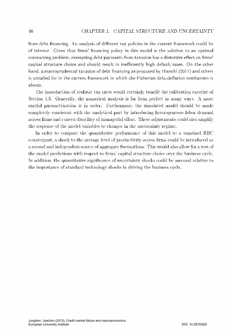
46 CHAPTER 1. CAPITAL STRUCTURE AND UNCERTAINTY
from debt nancing. An analysis of dierent tax policies in the current framework could be
of interest. Given that rms' nancing policy in this model is the solution to an optimal
contracting problem, exempting debt payments from taxation has a distortive eect on rms'
capital structure choice and should result in ineciently high default rates. On the other
hand, a macroprudential taxation of debt nancing as proposed by Bianchi (2011) and others
is uncalled for in the current framework in which the Fisherian debt-deation mechanism is
absent.
The introduction of realistic tax rates would certainly benet the calibration exercise of
Section 1.5. Generally, the numerical analysis is far from perfect in many ways. A more
careful parametrization is in order. Furthermore, the simulated model should be made
completely consistent with the analytical part by introducing heterogeneous labor demand
across rms and convex disutility of managerial eort. These adjustments could also amplify
the response of the model variables to changes in the uncertainty regime.
In order to compare the quantitative performance of this model to a standard RBC
counterpart, a shock to the average level of productivity across rms could be introduced as
a second and independent source of aggregate uctuations. This would also allow for a test of
the model predictions with respect to rms' capital structure choice over the business cycle.
In addition, the quantitative signicance of uncertainty shocks could be assessed relative to
the importance of standard technology shocks in driving the business cycle.
Jungherr, Joachim (2013), Credit market failure and macroeconomics European University Institute
DOI: 10.2870/929
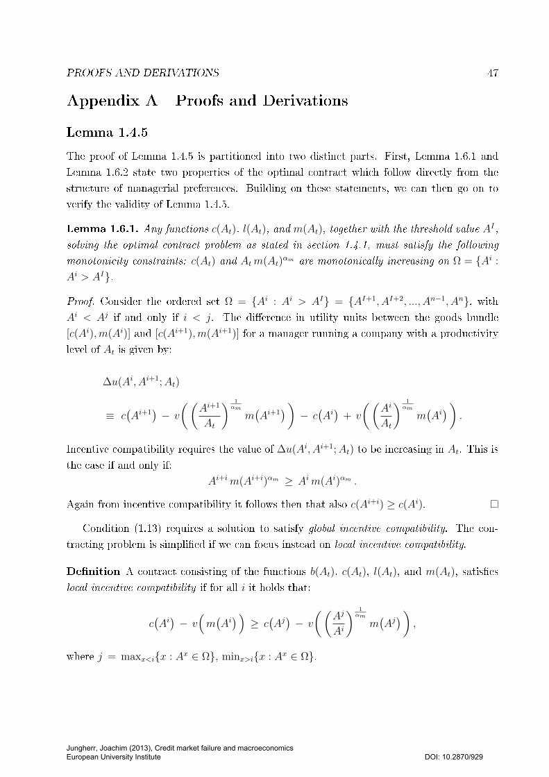
PROOFS AND DERIVATIONS 47
Appendix A Proofs and Derivations
Lemma 1.4.5
The proof of Lemma 1.4.5 is partitioned into two distinct parts. First, Lemma 1.6.1 and
Lemma 1.6.2 state two properties of the optimal contract which follow directly from the
structure of managerial preferences. Building on these statements, we can then go on to
verify the validity of Lemma 1.4.5.
Lemma 1.6.1. Any functions c(At), l(At), and m(At), together with the threshold value AI ,
solving the optimal contract problem as stated in section 1.4.1, must satisfy the following
monotonicity constraints: c(At) and Atm(At)αm are monotonically increasing on Ω = Ai :
Ai > AI.
Proof. Consider the ordered set Ω = Ai : Ai > AI = AI+1, AI+2, ..., An−1, An, withAi < Aj if and only if i < j. The dierence in utility units between the goods bundle
[c(Ai),m(Ai)] and [c(Ai+1),m(Ai+1)] for a manager running a company with a productivity
level of At is given by:
∆u(Ai, Ai+1;At)
≡ c(Ai+1
)− v
((Ai+1
At
) 1αm
m(Ai+1
))− c
(Ai)
+ v
((Ai
At
) 1αm
m(Ai))
.
Incentive compatibility requires the value of ∆u(Ai, Ai+1;At) to be increasing in At. This is
the case if and only if:
Ai+im(Ai+i)αm ≥ Aim(Ai)αm .
Again from incentive compatibility it follows then that also c(Ai+i) ≥ c(Ai).
Condition (1.13) requires a solution to satisfy global incentive compatibility. The con-
tracting problem is simplied if we can focus instead on local incentive compatibility.
Denition A contract consisting of the functions b(At), c(At), l(At), and m(At), satises
local incentive compatibility if for all i it holds that:
c(Ai)− v
(m(Ai) )≥ c
(Aj)− v
((Aj
Ai
) 1αm
m(Aj))
,
where j = maxx<ix : Ax ∈ Ω, minx>ix : Ax ∈ Ω.
Jungherr, Joachim (2013), Credit market failure and macroeconomics European University Institute
DOI: 10.2870/929

48 CHAPTER 1. CAPITAL STRUCTURE AND UNCERTAINTY
A manager should prefer truth-telling to misrepresenting her type by reporting the closest
unveried realizations below or above the true level of At. As Lemma 1.6.2 states, this is
indeed sucient for overall truth-telling.
Lemma 1.6.2. Local incentive compatibility implies global incentive compatibility.
Proof. Consider again the two productivity levels Ai, Ai+1 ∈ Ω. Local incentive compat-
ibility implies that Ai+im(Ai+i)αm ≥ Aim(Ai)αm . But in this case, the utility dierence
∆u(Ai, Ai+1;At) is increasing in At. That is, if the goods bundle [c(Ai+1),m(Ai+1)] is pre-
ferred to [c(Ai),m(Ai)] by a manager of type Ai+1, then a fortiori it is also preferred by any
manager of a rm with At > Ai+1. On the other hand, if the goods bundle [c(Ai),m(Ai)]
is preferred to [c(Ai+1),m(Ai+1)] by a manager of type Ai, then it is also preferred by any
manager of a rm with At < Ai.
Using the results of Lemma 1.6.1 and Lemma 1.6.2, we proceed to prove the individual
components of Lemma 1.4.5.
Proof. Clearly, the pooling allocation,
c(Ai) = c(Ai+1) and Aim(Ai)αm = Ai+1m(Ai+1)αm ,
does not violate incentive compatibility. Both, the local downward incentive compatibil-
ity constraint for Ai+1 and the local upward incentive compatibility constraint for Ai, are
simultaneoulsy binding in this case.
Now consider the possibility that:
c(Ai) < c(Ai+1) or Aim(Ai)αm < Ai+1m(Ai+1)αm .
If only one these two inequalities is strict, incentive compatibility is violated. If both inequal-
ities are strict, incentive compatibility may be satised. This is the separating allocation
considered in Lemma 1.4.5. In this case, the value of ∆u(Ai, Ai+1;At) from Lemma 1.6.1 is
strictly increasing in At.
Consider now the rst order condition for an optimal choice of c(An):
− p(An) + λ(An) − µ(An−1) = 0 ,
where p(An) is the probability of the event At = An. The Lagrange multipliers λ(An)
and µ(An−1) correspond to the downward local incentive compatibility constraint of An and
Jungherr, Joachim (2013), Credit market failure and macroeconomics European University Institute
DOI: 10.2870/929
PROOFS AND DERIVATIONS 49
upward local incentive compatibility for An−1, respectively. Obviously, upward incentive
compatibility does not apply to An and the participation constraint is slack, as follows from
Lemma 1.4.3. This optimality condition can only be satised if λ(An) > 0.
If An−1 and An are pooled, then we know that µ(An−1) > 0. If, on the other hand, An−1
and An are separated, then µ(An−1) = 0. Why?
From λ(An) > 0, it follows that:
∆u(An−1, An;An) = c(An)− v
(m(An) )− c
(An−1
)+ v
((An−1
An
) 1αm
m(An−1
) )= 0 .
Since ∆u(An−1, An;At) is strictly increasing in At for the separating allocation, it follows
that ∆u(An−1, An;An−1) < 0, and therefore µ(An−1) = 0.
If An−1 > AI+1, we can use µ(An−1) = ν(An−1) = 0 to derive again that λ(An−1) > 0.
Continuing in the manner outlined above, we can verify that λ(Ai) > 0 and ν(Ai) = 0 for
all Ai > AI+1, and µ(Ai) = 0 whenever Ai and Ai+1 are separated.
Lemma 1.4.6
Proof. To see this, we consider the range of unmonitored realizations Ai > AI and dene:
S(m(Ai), At
)≡ Ai kαkt l(Ai)αlm(Ai)αm + (1− δ) kt − wt l(A
i) − v((Ai
At
) 1αm
m(Ai) )
,
where labor demand l(Ai) is chosen as dened by Lemma 1.4.4. The function S(Ai, At
)gives
the social surplus which can be divided between rm managers and investors as specied by
the optimal contract for a given annoncement At = Ai and the true level of rm productivity
At. Incentive compatibility implies that rm investors receive S(m(Ai), Ai
)net of the rm
manager's information rent:
Ai kαkt l(Ai)αlm(Ai)αm + (1− δ) kt − wt l(Ai) − c(Ai)
= S(m(Ai), Ai
)−[c(Ai) − v
(m(Ai)
) ].
We know from Lemma 1.4.3 that these information rents are strictly increasing over the
unmonitored range Ai > AI . Furthermore, Lemma 1.4.5 states that the local downward
incentive compatibility constraint is always binding. This implies for the local increase of
Jungherr, Joachim (2013), Credit market failure and macroeconomics European University Institute
DOI: 10.2870/929

50 CHAPTER 1. CAPITAL STRUCTURE AND UNCERTAINTY
managers' information rents:
c(Ai+1) − v(m(Ai+1)
)−[c(Ai) − v
(m(Ai)
) ]= c(Ai) − v
(( Ai
Ai+1
) 1αm
m(Ai))−[c(Ai) − v
(m(Ai)
) ]= S
(m(Ai) , Ai+1
)− S
(m(Ai) , Ai
).
It is precisely the manager's option to misrepresent the rm's level of productivity by an-
nouncing Ai instead of Ai+1 which allows her to participate in the benet of a high realization
of At. These information rents add up as productivity levels grow over the unmonitored range
of productivity realizations Ω = AI+1, AI+2, AI+3, ..., An:
c(AI+1) − v(m(AI+1)
)= u ,
c(AI+2) − v(m(AI+2)
)= u + S
(m(AI+1) , AI+2
)− S
(m(AI+1) , AI+1
),
c(AI+3) − v(m(AI+3)
)= u + S
(m(AI+1) , AI+2
)− S
(m(AI+1) , AI+1
)+ S
(m(AI+2) , AI+3
)− S
(m(AI+2) , AI+2
),
...
c(An) − v(m(An)
)= u +
n−1∑j=I+1
S(m(Aj) , Aj+1
)− S
(m(Aj) , Aj
).
This allows us to express the expected payout to investors over the unmonitored range Ω as
a function of the surplus term S(m(Ai), Ai
)net of the rm manager's information rent:
n∑i=I+1
p(Ai)[Ai kαkt l(Ai)αlm(Ai)αm + (1− δ) kt − wt l(A
i) − c(Ai)]
=n∑
i=I+1
p(Ai)
[S(m(Ai) , Ai
)−[u +
i−1∑j=I+1
S(m(Aj) , Aj+1
)− S
(m(Aj) , Aj
) ] ].
Jungherr, Joachim (2013), Credit market failure and macroeconomics European University Institute
DOI: 10.2870/929
PROOFS AND DERIVATIONS 51
Rearranging the terms yields:
n∑i=I+1
p(Ai)
[S(m(Ai) , Ai
)−[u +
i−1∑j=I+1
S(m(Aj) , Aj+1
)− S
(m(Aj) , Aj
) ] ]
=[S(m(AI+1) , AI+1
)− u
] n∑j=I+1
p(Aj)
+[S(m(AI+2) , AI+2
)− S
(m(AI+1) , AI+2
) ] n∑j=I+2
p(Aj)
+[S(m(AI+3) , AI+3
)− S
(m(AI+2) , AI+3
) ] n∑j=I+3
p(Aj)
+ ...
+[S(m(An) , An
)− S
(m(An−1) , An
) ]p(An) .
The rst order condition of an optimal choice of m(Ai) now reads as:[αmA
i kαkt l(Ai)αlm(Ai)αm−1 − v′
(m(Ai)
) ] n∑j=i
p(Aj)
−[αmA
i kαkt l(Ai)αlm(Ai)αm−1 −
( Ai
Ai+1
) 1αm
v′(( Ai
Ai+1
) 1αm
m(Ai))] n∑
j=i+1
p(Aj)
=p(Ai)
[ 1− Pr(At ≤ Ai) ]
[αmA
i kαkt l(Ai)αlm(Ai)αm−1 − v′
(m(Ai)
) ]−[v′(m(Ai)
)−( Ai
Ai+1
) 1αm
v′(( Ai
Ai+1
) 1αm
m(Ai))]
= 0 . (1.21)
Pooling implies decreasing eort levels as rm productivity grows. The rst term in square
brackets must be strictly increasing in Ai in this case. At the same time, the second term
in square brackets gets smaller as Ai is growing and m(Ai) is falling due to the convexity of
v(m). If the hazard rate of F (A) is non-decreasing in Ai, then the rst order condition of
managerial eort can never be simultaneously satised for two pooled types. It follows that
in this case a complete separation of all unmonitored productivity types is optimal.
Jungherr, Joachim (2013), Credit market failure and macroeconomics European University Institute
DOI: 10.2870/929

52 CHAPTER 1. CAPITAL STRUCTURE AND UNCERTAINTY
Corollary 1.4.7
Proof. Consider the rst order condition of m(Ai) in equation (1.21) derived in the proof
to Lemma 1.4.6. For At = An, this equation is identical to equation (1.7). For all levels of
rm productivity AI < At < An, managerial eort is ineciently low. From Lemma 1.4.4 it
follows that rm output y(Ai) is distorted whenever managerial eort is ineciently low.
Proposition 1.4.8
Proof. Consider the consequences of increasing the threshold value AI from Ai−1 to Ai. The
probability of monitoring rises and so does the expected amount of monitoring costs. On the
upside, the range of unmonitored productivity states is reduced which lowers the extraction
of information rents by the rm manager.
For At = Ai+1, the rm manager gets now a utility level of u instead of:
c(Ai+1) − v(m(Ai+1)
)= u + S
(m(Ai) , Ai+1
)− S
(m(Ai) , Ai
).
Similarly, if At = Ai+2, then the rm manager's utility is now given by:
c(Ai+2) − v(m(Ai+2)
)= u + S
(m(Ai+1) , Ai+2
)− S
(m(Ai+1) , Ai+1
),
instead of:
c(Ai+2) − v(m(Ai+2)
)= u + S
(m(Ai) , Ai+1
)− S
(m(Ai) , Ai
)+ S
(m(Ai+1) , Ai+2
)− S
(m(Ai+1) , Ai+1
).
Information rents are reduced over the entire range of unmonitored productivity states.
Accordingly, the optimal threshold value AI is characterized by the following two conditions:
p(AI)G(y(AI)
)≤[S(m(AI) , AI+1
)− S
(m(AI) , AI
) ] n∑j=I+1
p(Aj) ,
together with:
p(AI+1)G(y(AI+1)
)>[S(m(AI+1) , AI+2
)− S
(m(AI+1) , AI+1
) ] n∑j=I+2
p(Aj) .
It pays o to monitor AI , but the additional costs of increasing the monitored range further
Jungherr, Joachim (2013), Credit market failure and macroeconomics European University Institute
DOI: 10.2870/929

MODEL SOLUTION AND SIMULATION 53
exceed the associated reduction in information rents. Generally, we will not always have
such an interior solution A1 < AI < An. But if it exists, then it is straightforward to see
that a high value of G(y(Ai)
)lowers the optimal threshold value AI . What is the role of the
output elasticity αm? We can rewrite:
S(m(Ai) , Ai+1
)− S
(m(Ai) , Ai
)= v
(m(Ai)
)− v(( Ai
Ai+1
) 1αm
m(Ai)).
From equation (1.21), we know that m(Ai) is strictly increasing in αm which drives up
information rents. However, there is one opposing force as:
∂
∂ αm
[( Ai
Ai+1
) 1αm
]> 0 .
But note that as ∆A = Ai−Ai−1 becomes small enough, this eect loses power. Consequently,
for a suciently small step size ∆A rm managers' information rents are increasing in αm
which renders monitoring more attractive.
Appendix B Model Solution and Simulation
In this appendix, I rst lay out the algorithm for numerically solving the model and then explain how it issimulated to generate articial data on the behavior of real and nancial variables over time.
Solving the Model
Optimal Contract
At the heart of the model lies the optimal contract between investors and managers as a solution to theproblem laid out in (1.12)-(1.15). The optimal choice of managerial eort is described by the respective rstorder conditions given above. Manager compensation is then pinned down by the remaining incentive andparticipation constraints. The optimal choice of AI needs to be calculated using simple numerical methods.
In a rst step, I solve the optimal contract conditional on some given threshold value AI . The expectedaggregate payout to investors implied by the solution to this constrained maximization problem is thencompared across all dierent threshold values AI . The highest value gives the solution to the optimalcontract problem specied in (1.12)-(1.15). A high value of n is desirable in order to get a ne grid for Atwhich allows for a precise identication of AI . The number n is set to 100.
The optimal contract is solved once for each probability distribution F (At). It is not necessary to solveit for dierent values of rm capital because the optimal contract of the model used in the numerical analysisis scale-independent. Due to constant returns to scale in the production technology and managers' lineardisutility of eort, the solution to m(Ai) and c(Ai) is just scaled up or down by changes in capital and laborinput, while the optimal threshold value AI remains unchanged. Given a solution for some arbitrary valuesof capital kt and labor lt, the values for m(Ai) and c(Ai) respond to changes in
X = kαkt lαlt
Jungherr, Joachim (2013), Credit market failure and macroeconomics European University Institute
DOI: 10.2870/929
54 CHAPTER 1. CAPITAL STRUCTURE AND UNCERTAINTY
according to:
m′(Ai) =
(X ′
X
) 11−αm
m(Ai) , and: c′(Ai) =
(X ′
X
) 11−αm
c(Ai) .
Equilibrium
The recursive optimization problem of households is given by:
V (W, s) = maxW ′
log
(W − 1
R∗′(W ′ − w′ l
))+∑s′
π(s′|s)β V (W ′, s′) ,
where W is the household's current wealth level:
W = w l + (e+ d)R∗ .
Note that in equilibrium the portfolio of the representative household is perfectly diversied and she earnsthe return R∗ with certainty. Next period's wealth level W ′ depends on savings today, W − c, and on nextperiod's prices R∗′ and w′. These prices depend on next period's exogenous state of uncertainty s, which isknown at the time of the household's savings decision, and on next period's aggregate stock of capital k′.Taking as given the stock of aggregate capital k′ in the economy as a function of the state variables W ands, the households solves the recursive problem outlined above. In equilibrium, the household's savings policymust be equal to the assumed function of aggregate capital:
k(W, s) =1
R∗′(W ′(W, s) − w′ l
).
The function k(W, s) is initially specied by an arbitrary guess. The household's savings decision is thencalculated and used to update our initial guess for k(W, s). This procedure is iteratively repeated until ourguess and the actual solution converge.
Simulation
Uncertainty
The source of all variation in the simulated model economies is time-varying uncertainty about rm pro-ductivity At. I assume F (At) to be truncated lognormal with a constant mean of 1 and a state-dependentstandard deviation of σt. The exogenous state of rm-level uncertainty is specied as a discrete Markovchain with nine distinct levels.
It is constructed as follows. I calculate the probability values of a lognormal distribution with a meanvalue of 1 and a standard deviation of 0.84 on a grid of values of rm productivity At. This grid isencompassing values one standard deviation below and above the mean: it is limited by the boundariesA1 = 0.16 and An = 1.84. I proceed to create the corresponding probability values of a truncated lognormaldistribution by scaling up the probability mass p(Ai) on this grid such that:
n∑i=1
p(Ai) = 1 .
Due to the asymmetry of the lognormal density, the resulting probability distribution will generally not havea mean value of 1 anymore. In order to x this, I multiply the discrete support of At: A1, A2, ..., An, by
Jungherr, Joachim (2013), Credit market failure and macroeconomics European University Institute
DOI: 10.2870/929
MODEL SOLUTION AND SIMULATION 55
the factor:
f =
[ n∑i=1
p(Ai)Ai]−1
.
The unchanged values of p(Ai) together with support fA1, fA2, ..., fAn gives a truncated lognormal dis-tribution F (At) which has a mean value of 1 and a standard deviation of 0.46. This will be the probabilitydistribution for the average state of rm-level uncertainty.
The other states of uncertainty dier from the average level by the variable D(s). This variable increasesor diminishes the support and the variance of F (At) in the following way. The original grid, encompassingvalues from A1 = 0.16 until An = 1.84, is expanded or truncated across dierent states of uncertaintyaccording to: A1(s) = 0.16−D(s) and An(s) = 1.84 +D(s). The probability values p(Ai) for this grid arethe same as for the average state of uncertainty. In order to normalize the mean value of this distribution to1, the discrete support of At: A1, A2, ..., An is multiplied by the factor f(s). The unchanged values of p(Ai)together with support f(s)A1(s), f(s)A2(s), ..., f(s)An(s) gives again a truncated lognormal distributionwith mean 1 and a standard deviation σt which is higher (smaller) than 0.46 if D(s) is positive (negative).
In order to dene the variation of rm-level risk over time, I specify D(s) as a discrete-valued Markovchain. The method of Tauchen (1986) is used to approximate an AR(1) process with an unconditional mean0 and a standard deviation of the white noise process of 0.034. The persistence parameter is chosen as 0.97,and the grid encompasses one times the unconditional standard deviation below and above the unconditionalmean 0. The number of grid points is set to 9. The nine resulting exogenous states of uncertainty featurethe following levels of standard deviation: 0.37, 0.39, 0.41, 0.43, 0.46, 0.48, 0.50, 0.53, 0.55.
Impulse Response Functions
In order to measure the typical response of real and nancial variables to an increase in rm-level uncertainty,the model is simulated for 10,000 dierent model economies over a time period of 180 quarters each. Duringthe rst 50 quarters, each simulated model economy is following an individual stochastic time path. In the50th quarter, agents across all 10,000 simulated economies learn that the exogenous uncertainty state willjump up by two levels in the next period (or will be equal to the highest value on the grid in case the currentstate of uncertainty is already on the 8th or 9th level). Investment and consumption respond on impact,while the other endogenous variables react to the shock starting from quarter 51 onwards. For all remainingtime periods, the exogenous state is following an individual time path again for each model economy. Impulseresponses are generated by taking the average of the variables of interest at a given point in time across all10,000 economies.
Jungherr, Joachim (2013), Credit market failure and macroeconomics European University Institute
DOI: 10.2870/929

56 CHAPTER 1. CAPITAL STRUCTURE AND UNCERTAINTY
Bibliography
Abel, Andrew B. (1983). `Optimal Investment Under Uncertainty,' The American Economic Review, Vol.73(1), pp. 228-233.
Adrian, Tobias, Paolo Colla, and Hyun Song Shin (2013). `Which Financial Frictions? Parsing the Evidencefrom the Financial Crisis of 2007-9.' in: D. Acemoglu, J. Parker & M. Woodford (ed.), NBER Macroeco-
nomics Annual 2012, Vol. 27, pp. 159-214, University of Chicago Press.
Aghion, Philippe and Patrick Bolton (1992). `An Incomplete Contracts Approach to Financial Contracting,'The Review of Economic Studies, Vol. 59(3), pp. 473-494.
Arellano, Cristina, Yan Bai, and Patrick Kehoe (2012). `Financial Frictions and Fluctuations in Volatility,'Federal Reserve Bank of Minneapolis Research Department Sta Report no. 466, July 2012.
Atkeson, Andrew and Harold Cole (2008). `A Dynamic Theory of Optimal Capital Structure and ExecutiveCompensation,' mimeo, January 2008.
Bachmann, Rüdiger, Steen Elstner, and Eric R. Sims (2010). `Uncertainty and Economic Activity: Evi-dence from Business Survey Data,' NBER Working Paper no. 16143, June 2010.
Bachmann, Rüdiger and Christian Bayer (2011). `Investment Dispersion and the Business Cycle,' NBERWorking Paper no. 16861, February 2011.
Bachmann, Rüdiger and Giuseppe Moscarini (2011). `Business Cycles and Endogenous Uncertainty,' mimeo,July 2011.
Bachmann, Rüdiger and Christian Bayer (2013). ` Wait-and-See Business Cycles?' Journal of Monetary
Economics, Vol. 60(6), pp. 704-719.
Baker, George P. and Brian J. Hall (2004). `CEO Incentives and Firm Size,' Journal of Labor Economics,Vol. 22(4), pp. 767-798.
Baker, Scott, Nicholas Bloom, and Steven Davis (2013). `Measuring Economic Policy Uncertainty,' ChicagoBooth Research Paper no. 13-02, January 2013.
Basu, Susanto (1996). `Procyclical Productivity: Increasing Returns or Cyclical Utilization?' The QuarterlyJournal of Economics, Vol. 111(3), pp. 719-751.
Basu, Susanto and Brent Bundick (2012). `Uncertainty Shocks in a Model of Eective Demand,' NBERWorking Paper no. 18420, September 2012.
Bebchuk, Lucian and Yaniv Grinstein (2005). `The Growth of Executive Pay,' Oxford Review of Economic
Policy, Vol. 21(2), pp. 283-303.
Bernanke, Ben S. and Mark Gertler (1989). `Agency Costs, Net Worth, and Business Fluctuations,' TheAmerican Economic Review, Vol. 79(1), pp. 14-31.
Bernanke, Ben S., Mark Gertler, and Simon Gilchrist (1999). `The Financial Accelerator in a QuantitativeBusiness Cycle Framework,' in: J. B. Taylor & M. Woodford (ed.), Handbook of Macroeconomics, Ed. 1,Vol. 1, Chapter 21, pp. 1341-1393, Elsevier.
Bernanke, Ben S. (2010). `Restoring the Flow of Credit to Small Businesses,' Remarks at the Federal Re-serve Meeting Series: `Addressing the Financing Needs of Small Businesses', Washington, D.C., U.S., July12, 2010.
Biais, Bruno and Catherine Casamatta (1999). `Optimal Leverage and Aggregate Investment,' The Journalof Finance, Vol. 54(4), pp. 1291-1323.
Jungherr, Joachim (2013), Credit market failure and macroeconomics European University Institute
DOI: 10.2870/929

BIBLIOGRAPHY 57
Biais, Bruno, Thomas Mariotti, Guillaume Plantin, and Jean-Charles Rochet (2007). `Dynamic SecurityDesign: Convergence to Continuous Time and Asset Pricing Implications,' The Review of Economic Studies,Vol. 74(2), pp. 345-390.
Bianchi, Javier (2011). `Overborrowing and Systemic Externalities in the Business Cycle,' The American
Economic Review, Vol. 101(7), pp. 3400-3426.
Bloom, Nicholas and John Van Reenen (2007). `Measuring and Explaining Management Practices acrossFirms and Countries,' The Quarterly Journal of Economics, Vol. 122(4), pp. 1351-1408.
Bloom, Nicholas (2009). `The Impact of Uncertainty Shocks,' Econometrica, Vol. 77(3), pp. 623-685.
Bloom, Nicholas, Max Floetotto, Nir Jaimovich, Itay Saporta-Eksten, and Stephen J. Terry (2012). `ReallyUncertain Business Cycles,' NBER Working Paper no. 18245, July 2012.
Bloom, Nicholas, Benn Eifert, Aprajit Mahajan, David McKenzie, and John Roberts (2013). `Does Man-agement Matter? Evidence from India,' The Quarterly Journal of Economics, Vol. 128(1), pp. 1-51.
Boyd, John H. and Bruce D. Smith (1998). `The Evolution of Debt and Equity Markets in Economic De-velopment,' Economic Theory, Vol. 12(3), pp. 519-560.
Bradley, Michael, Gregg A. Jarrell, and E. Han Kim (1984). `On the Existence of an Optimal Capital Struc-ture: Theory and Evidence,' The Journal of Finance, Vol. 39(3), pp. 857-878.
Bris, Arturo, Ivo Welch, and Ning Zhu (2006). `The Costs of Bankruptcy: Chapter 7 Liquidation versusChapter 11 Reorganization,' The Journal of Finance, Vol. 61(3), pp. 1253-1303.
Brunnermeier, Markus K. and Yuliy Sannikov (2010). `A Macroeconomic Model with a Financial Sector,'mimeo, May 2010.
Burnside, Craig, Martin Eichenbaum, and Sergio Rebelo (1993). `Labor Hoarding and the Business Cycle,'The Journal of Political Economy, Vol. 101(2), pp. 245-273.
Burnside, Craig and Martin Eichenbaum (1996). `Factor-Hoarding and the Propagation of Business-CycleShocks,' The American Economic Review, Vol. 86(5), pp. 1154-1174.
Campbell, John Y., Martin Lettau, Burton G. Malkiel, and Yexiao Xu (2001). `Have Individual Stocks Be-come More Volatile? An Empirical Exploration of Idiosyncratic Risk,' The Journal of Finance, Vol. 56(1),pp. 1-43.
Campbell, John Y. and Glen B. Taksler (2003). `Equity Volatility and Corporate Bond Yields,' The Journalof Finance, Vol. 58(6), pp. 2321-2350.
Carlstrom, Charles T. and Timothy S. Fuerst (1997). `Agency Costs, Net Worth, and Business Fluctuations:A Computable General Equilibrium Analysis,' The American Economic Review, Vol. 87(5), pp. 893-910.
Chang, Chun (1992). `Capital Structure as an Optimal Contract between Employees and Investors,' TheJournal of Finance, Vol. 47(3), pp. 1141-1158.
Chang, Chun (1993). `Payout Policy, Capital Structure, and Compensation Contracts when Managers ValueControl,' The Review of Financial Studies, Vol. 6(4), pp. 911-933.
Chari, Varadarajan V., Patrick J. Kehoe, and Ellen R. McGrattan (2007). `Business Cycle Accounting,'Econometrica, Vol. 75(3), pp. 781-836.
Christiano, Lawrence, Roberto Motto, and Massimo Rostagno (2013). `Risk Shocks,' NBER Working Paperno. 18682, January 2013.
Chugh, Sanjay K. (2012). `Firm Risk and Leverage Based Business Cycles,' mimeo, July 2012.
Jungherr, Joachim (2013), Credit market failure and macroeconomics European University Institute
DOI: 10.2870/929
58 CHAPTER 1. CAPITAL STRUCTURE AND UNCERTAINTY
Clementi, Gian Luca and Thomas Cooley (2010). `Executive Compensation: Facts,' mimeo, July 2010.
Cole, Harold (2011). `Self-Enforcing Stochastic Monitoring and the Separation of Debt and Equity Claims,'mimeo, November 2011.
Covas, Francisco and Wouter J. Den Haan (2011). `The Role of Debt and Equity Finance Over the BusinessCycle,' mimeo, January 2011.
Davis, Steven J., John Haltiwanger, Ron Jarmin, and Javier Miranda (2007). `Volatility and Dispersion inBusiness Growth Rates: Publicly Traded versus Privately Held Firms,' in: D. Acemoglu, K. Rogo & M.Woodford (ed.), NBER Macroeconomics Annual 2006, Vol. 21, pp. 107-180, The MIT Press.
DeMarzo, Peter M. and Yuliy Sannikov (2006). `Optimal Security Design and Dynamic Capital Structurein a Continuous-Time Agency Model,' The Journal of Finance, Vol. 61(6), pp. 2681-2724.
DeMarzo, Peter M. and Michael J. Fishman (2007). `Optimal Long-Term Financial Contracting,' The Re-
view of Financial Studies, Vol. 20(6), pp. 2079-2128.
Dewatripont, Mathias and Jean Tirole (1994). `A Theory of Debt and Equity: Diversity of Securities andManager-Shareholder Congruence,' The Quarterly Journal of Economics, Vol. 109(4), pp. 1027-1054.
Diamond, Douglas W. (1984). `Financial Intermediation and Delegated Monitoring,' The Review of Eco-
nomic Studies, Vol. 51(3), pp. 393-414.
Dorofeenko, Victor, Gabriel S. Lee and Kevin D. Salyer (2008). `Time-varying Uncertainty and the CreditChannel,' Bulletin of Economic Research, Vol. 60(4), pp. 375-403.
Duygan-Bump, Burcu, Alexey Levkov, and Judit Montoriol-Garriga (2011). `Financing Constraints andUnemployment: Evidence from the Great Recession,' Federal Reserve Bank of Boston Working Paper no.QAU10-6, December 2011.
Eisfeldt, Andrea L. and Adriano A. Rampini (2006). `Capital Reallocation and Liquidity,' Journal of Mon-
etary Economics, Vol. 53(3), pp. 369-399.
Eisfeldt, Andrea L. and Adriano A. Rampini (2008). `Managerial Incentives, Capital Reallocation, and theBusiness Cycle,' Journal of Financial Economics, Vol. 87(1), pp. 177-199.
Fama, Eugene F. and Kenneth R. French (2005). `Financing Decisions: Who Issues Stock?' Journal of
Financial Economics, Vol. 76(3), pp. 549-582.
Fernald, John (2012). `Productivity and Potential Output before, during, and after the Great Recession,'Federal Reserve Bank of San Francisco Working Paper no. 2012-18, September 2012.
Fernández-Villaverde, Jesús, Pablo Guerrón-Quintana, Juan F. Rubio-Ramírez, and Martin Uribe (2011).`Risk Matters: The Real Eects of Volatility Shocks,' The American Economic Review, Vol 101(6), pp.2530-2561.
Fluck, Zsuzsanna (1998). `Optimal Financial Contracting: Debt versus Outside Equity,' The Review of
Financial Studies, Vol. 11(2), pp. 383-418.
Friend, Irwin and Larry H.P. Lang (1988). `An Empirical Test of the Impact of Managerial Self-interest onCorporate Capital Structure,' The Journal of Finance, Vol. 43(2), pp. 271-281.
Gabaix, Xavier and Augustin Landier (2008). `Why Has CEO Pay Increased So Much?' The Quarterly
Journal of Economics, Vol. 123(1), pp. 49-100.
Gale, Douglas and Martin Hellwig (1985). `Incentive-Compatible Debt Contracts. The One-Period Prob-lem,' The Review of Economic Studies, Vol. 52(4), pp. 647-663.
Jungherr, Joachim (2013), Credit market failure and macroeconomics European University Institute
DOI: 10.2870/929
BIBLIOGRAPHY 59
Giesecke, Kay, Francis A. Longsta, Stephen Schaefer, and Ilya Strebulaev (2013). `Macroeconomic Eectsof Corporate Default Crises: A Long-Term Perspective,' NBER Working Paper no. 17854, July 2013.
Gilchrist, Simon, Jae W. Sim, and Egon Zakraj²ek (2010). `Uncertainty, Financial Frictions, and InvestmentDynamics,' mimeo, September 2010.
Gilchrist, Simon and Egon Zakraj²ek (2012). `Credit Spreads and Business Cycle Fluctuations,' AmericanEconomic Review, Vol. 102(4), pp. 1692-1720.
Gomes, João F., Amir Yaron, and Lu Zhang (2003). `Asset Prices and Business Cycles with Costly ExternalFinance,' Review of Economic Dynamics, Vol. 6, pp. 767-788.
Gomes, João F. and Lukas Schmid (2010). `Equilibrium Credit Spreads and the Macroeconomy,' mimeo,July 2010.
Gourio, François (2008). `Estimating Firm-level Risk,' mimeo, October 2008.
Greenwood, Jeremy, Juan M. Sanchez, and Cheng Wang (2010). `Financing Development: The Role ofInformation Costs,' American Economic Review, Vol. 100(4), pp. 1875-1891.
Greenwood, Jeremy, Juan M. Sanchez, and Cheng Wang (2013). `Quantifying the Impact of Financial De-velopment on Economic Development,' Review of Economic Dynamics, Vol. 16(1), pp. 194-215.
Hartman, Richard (1972). `The Eects of Price and Cost Uncertainty on Investment,' Journal of EconomicTheory, Vol. 5, pp. 258-266.
Higson, Chris, Sean Holly, and Paul Kattuman (2002). `The Cross-sectional Dynamics of the US BusinessCycle: 1950-1999,' Journal of Economic Dynamics and Control, Vol. 26(9), pp. 1539-1555.
Higson, Chris, Sean Holly, Paul Kattuman, and Stelios Platis (2004) `The Business Cycle, MacroeconomicShocks and the Cross-Section: The Growth of UK Quoted Companies,' Economica, Vol. 71(282) pp. 299-318.
Jensen, Michael C. and William H. Meckling (1976), `Theory of the Firm: Managerial Behavior, AgencyCosts and Ownership Structure,' Journal of Financial Economics, Vol. 3(4), pp. 305-360.
Jensen, Michael C. (1986). `Agency Costs of Free Cash Flow, Corporate Finance, and Takeovers,' TheAmerican Economic Review, Volume 76(2), pp. 323-329.
Jermann, Urban and Vincenzo Quadrini (2012). `Macroeconomic Eects of Financial Shocks,' The AmericanEconomic Review, Volume 102(1), pp. 238-271.
Kiyotaki, Nobuhiro and John Moore (1997). `Credit Cycles,' Journal of Political Economy, Vol. 105(2), pp.211-248.
Korteweg, Artur (2010). `The Net Benets to Leverage,' Journal of Finance, Vol. 65(6), pp. 2137-2170.
Koufopoulos, Kostas (2009). `Optimal Securities under Adverse Selection and Moral Hazard,' Journal ofMathematical Economics, Vol. 45(5), pp. 341-360.
Lang, Jan Hannes (2012). `The Role of Uncertainty Shocks in US Business Cycles,' mimeo, August 2012.
Leduc, Sylvain and Zheng Liu (2013). `Uncertainty Shocks are Aggregate Demand Shocks,' Federal ReserveBank of San Francisco Working Paper no. 2012-10, January 2013.
Levy, Amnon and Christopher Hennessy (2007). `Why Does Capital Structure Choice Vary with Macroeco-nomic Conditions?' Journal of Monetary Economics, Vol. 54(6), pp. 1545-1564.
Jungherr, Joachim (2013), Credit market failure and macroeconomics European University Institute
DOI: 10.2870/929
60 CHAPTER 1. CAPITAL STRUCTURE AND UNCERTAINTY
Lorenzoni, Guido (2008). `Inecient Credit Booms,' The Review of Economic Studies, Vol. 75(3), pp. 809-833.
Meisenzahl, Ralf R. (2011). `Verifying the State of Financing Constraints: Evidence from US Business CreditContracts,' Federal Reserve Board Finance and Economics Discussion Series Working Paper no. 2011-04,January 2011.
Merton, Robert C. (1974). `On The Pricing of Corporate Debt: The Risk Structure of Interest Rates,' TheJournal of Finance, Vol. 29(2), pp. 449-470.
Morellec, Erwan, Boris Nikolov, and Norman Schürho (2012). `Corporate Governance and Capital Struc-ture Dynamics,' The Journal of Finance, Vol. 67(3), pp. 803-848.
Narita, Futoshi (2011). `Hidden Actions, Risk-Taking, and Uncertainty Shocks,' mimeo, February 2011.
Nikolov, Boris and Norman Schürho (2012). `Testing Dynamic Agency Theory via Structural Estimation,'mimeo, March 2012.
Oi, Walter Y. (1961). `The Desirability of Price Instability under Perfect Competition,' Econometrica, Vol.29(1), pp. 58-64.
Orlik, Anna and Laura Veldkamp (2013). `Understanding Uncertainty Shocks,' mimeo, February 2013.
Osotimehin, Sophie (2013). `Aggregate Productivity and the Allocation of Resources over the Business Cy-cle,' mimeo, August 2013.
Quadrini, Vincenzo (2011). `Financial Frictions in Macroeconomic Fluctuations,' Federal Reserve Bank of
Richmond Economic Quarterly, Vol. 97(3), pp. 209-254.
Ross, Stephen A. (1973). `The Economic Theory of Agency: The Principal's Problem,' American Economic
Review, Vol. 63(2), pp. 134-139.
Schaal, Edouard (2012). `Uncertainty, Productivity and Unemployment in the Great Recession,' mimeo,January 2012.
Shourideh, Ali and Ariel Zetlin-Jones (2012). `External Financing and the Role of Financial Frictions overthe Business Cycle: Measurement and Theory,' mimeo, June 2012.
Tauchen, George (1986). `Finite State Markov-Chain Approximations to Univariate and Vector Autoregres-sions,' Economics Letters, Vol. 20, pp. 177-181.
Terviö, Marko (2008). `The Dierence that CEOs Make: An Assignment Model Approach,' The American
Economic Review, Vol. 98(3), pp. 642-668.
Townsend, Robert M. (1979). `Optimal Contracts and Competitive Markets with Costly State Verication,'Journal of Economic Theory, Vol. 21, pp. 265-293.
Van Nieuwerburgh, Stijn and Laura Veldkamp (2006). `Learning Asymmetries in Real Business Cycles,'Journal of Monetary Economics, Vol. 53(4), pp. 753-772.
Veldkamp, Laura (2005). `Slow Boom, Sudden Crash,' Journal of Economic Theory, Vol. 124(2), pp. 230-257.
Zwiebel, Jerey (1996). `Dynamic Capital Structure under Managerial Entrenchment,' The American Eco-
nomic Review, Vol. 86(5), pp. 1197-1215.
Jungherr, Joachim (2013), Credit market failure and macroeconomics European University Institute
DOI: 10.2870/929
Chapter 2
Bank Opacity and Endogenous
Uncertainty
2.1 Introduction
It seems to be a widely held view that the nancial system is particularly opaque. Indeed,
empirical evidence suggests that the protability of banks is harder to predict for outsiders
than the performance of non-nancial rms.1 Also in the aftermath of the 2008 nancial
crisis, insucient transparency has frequently been put forward as an important factor to
understand the origins and severity of the crisis.2 Consequently, policy has implemented
measures which are meant to improve public disclosure and bank transparency. The Dodd-
Frank Act of 2010 requires the Federal Reserve to publish a summary of the results of its
annual supervisory stress test of large bank holding companies. The published stress test
results include company-specic measures of risk exposure to selected scenarios. Pillar 3 of
the Basel Accords species public disclosure requirements for banks including information on
asset holdings and risk exposure. However, these policy measures explicitly did not constitute
an attempt to achieve a maximum level of transparency. The Squam Lake Report (2010)
acknowledges that it is important to protect proprietary business models and incentives
to innovate. Public disclosure of a rm's positions also raises concerns about predatory or
1See Morgan (2002), Hirtle (2006), Iannotta (2006), or Jones, Lee and Yeager (2012). Flannery, Kwanand Nimalendran (2004) nd banks not to be more opaque than non-nancial rms.
2The Squam Lake Report (2010) identies a critical lack of information about the risk exposure of nancialrms. The authors argue in favor of access for regulators to more information about banks' asset positionsand risk sensitivities. They also advocate the release of this information to the public with a suitable timelag. Bernanke (2010) agrees with the perception of opaqueness as one of the structural weaknesses in theshadow banking system.
61
Jungherr, Joachim (2013), Credit market failure and macroeconomics European University Institute
DOI: 10.2870/929
62 CHAPTER 2. BANK OPACITY
copycat trading by competitors. Implemented disclosure requirements reect this warning
by specifying deliberate time lags and a suitable degree of aggregation.
What does economic theory have to say about this question? In order to justify manda-
tory disclosure rules for banks, one needs to show that in the absence of regulation banks
choose to transmit too little information to the public. So what is special about banks
that makes them more opaque than non-nancial rms? What exactly are the external-
ities which give rise to a need for policy intervention? And what is the optimal level of
bank transparency? Existing contributions have focused on the particularly fragile liabilities
structure of banks and the role of transparency in preventing (or triggering) socially costly
banking crises. This paper adopts a dierent perspective and points to the asset side of
banks' balance sheets. In this model, banks are special because the product they are selling
to households is superior information about investment opportunities. Intransparent balance
sheets turn this public good into a marketable private commodity. Unilateral disclosure of
this information translates into a competitive disadvantage. Complete bank opacity is the
only equilibrium in the absence of policy intervention. Households do value public infor-
mation as it reduces aggregate uncertainty, but the market does not punish intransparent
banks. Mandatory disclosure rules can improve upon the market allocation because of the
public good character of banks' information.
Preview of the Model and Results
The banking sector is modelled as a simple duopoly with Bertrand competition. Two banks
compete for households' savings. Banks use these funds to invest in some combination of
riskless and risky investment projects. The more information a bank has about the future
protability of risky investment projects, the better and safer its portfolio choice will be.
This information is not only valuable for banks, which choose the composition of households'
investment portfolio, but also for households, who have to decide on how much to save and
thereby on the aggregate size of their investment portfolio.
If households can choose between investing in a fully transparent bank, which shares all
its information with the public, and a competitor bank, which remains opaque, then each
single household will paradoxically choose the latter. Why is it that the socially harmful
behavior of opaque banks gets rewarded by the market? The opaque bank knows more about
future investment opportunities than its transparent competitor and therefore its portfolio
choice will be better. The opaque bank can rely on its private information as well as on the
information shared by its transparent competitor, while the transparent bank only knows
its own information and does not participate in its rival's information set. In this situation,
Jungherr, Joachim (2013), Credit market failure and macroeconomics European University Institute
DOI: 10.2870/929
2.1. INTRODUCTION 63
households face a prisoner's dilemma: if they could coordinate to invest only in transparent
banks, each one of them would be better o, as in this case there would be no incentive for
banks to hide information from the public. But once a bank reduces disclosure, it earns a
competitive advantage over the transparent rival because of its superior information and it
becomes protable for households to invest in the opaque bank. Competition between the
two banks results in a race to the bottom which leads to complete bank opacity and a high
degree of aggregate uncertainty for households.
Policy measures can improve upon this market outcome by imposing minimum disclo-
sure requirements on banks. Complete disclosure is socially undesirable as this eliminates
all private incentives to acquire costly information. The social planner chooses optimal
bank transparency by trading o the benets of reducing aggregate uncertainty for house-
holds (Blackwell eect3) against the incentives for costly information acquisition (Grossman-
Stiglitz eect4).
Related Literature
The main argument used in support of mandatory public disclosure is improved market
discipline. Public information about the expected protability of individual banks helps
nancial markets to allocate resources eciently across nancial rms. Allegedly, it also
prevents bank managers from excessive risk taking and thereby contributes to nancial sta-
bility. These points seem to be very much in line with plain common sense and this might
be the reason why economic research has tended to focus on the potential costs of nancial
transparency rather than on its social benets.5 There are only a few examples of formal
models which explain why market forces on their own are not capable of creating a sucient
level of bank transparency.
These models are generally of recent vintage. Chen and Hasan (2006) show that bank
managers may want to delay disclosure in order to avoid ecient bank runs. Mandatory
disclosure rules can restore market discipline in this case. An important assumption here
is that bank managers cannot commit to a pre-selected timing of disclosure. This would
remove the need for policy intervention.
The experience of the Financial Crisis 2007-2008 is reected in an increased interest in
3Blackwell (1951) shows that for a single decision maker more information about fundamentals is alwaysdesirable.
4Grossman and Stiglitz (1976, 1980) famously demonstrate that full transparency eliminates all incentivesfor costly information acquisition.
5This is true also for two recent review articles on the trade-os involved in nancial transparency. SeeLandier and Thesmar (2011) and Goldstein and Sapra (2012).
Jungherr, Joachim (2013), Credit market failure and macroeconomics European University Institute
DOI: 10.2870/929

64 CHAPTER 2. BANK OPACITY
the topic. In Bouvard, Chaigneau, and de Motta (2012), depositors know the health of the
average bank in the economy but only a regulator knows the asset quality of each individual
bank. During normal times, informational opacity prevents inecient bank runs. However,
if investors observe that the nancial sector is hit by a crisis, public information about
individual banks is desirable in order to prevent a run on the whole nancial system. Only
the regulator can provide this information, as banks' announcements are not veriable. A
similar result is found by Spargoli (2012). During normal times, there is no policy need as
banks with high quality assets can separate themselves from low quality banks. However,
during a nancial crisis separation becomes too costly and nancial markets are unable to
discriminate between banks of dierent quality.
Also Alvarez and Barlevy (2012) study an endogenous lack of information about the
location and size of bank losses. Banks form a nancial network in this model which exposes
them to the credit risk of their counterparties. This gives rise to an information externality
as information about the nancial health of one bank is also valuable with respect to the risk
exposure of its counterparties. Crucial for the authors' results is an exogenous xed cost of
public disclosure.
The contributions cited above do not model banks' portfolio choice and there is no feed-
back eect from public disclosure to a bank's market share and the quality of its assets. In
contrast, this paper introduces the problem of costly information acquisition to the analysis
which endogenizes the costs of public disclosure.
As mentioned above, the social costs of bank transparency have been studied at least as
extensively as the potential benets. For instance, Moreno and Takalo (2012) nd that neg-
ative spillovers of bank failures result in an oversupply of voluntary disclosure. If anything,
policy should induce banks to disclose less information to the public than they would like to.
Also Dang, Gorton, Holmström and Ordoñez (2013) warn of the perils of bank transparency.
In their model, it is precisely the role of banks to collect socially valuable information about
asset quality without disclosing it to the public. The negative role of public information in
this model is related to Hirshleifer (1971).6 Consumers are exposed to liqudity shocks. This
makes them unwilling to invest in risky projects if information about project losses become
public. A bank which can hide these project losses from the public is able to shut down the
Hirshleifer eect and to channel households' savings to investment projects. Banks allow
households to share both the risks of production and of stochastic liquidity needs. More
opacity is better in this environment.
6Hirshleifer (1971) shows that disclosure is socially harmful whenever its primary eect is to redistributewealth among agents.
Jungherr, Joachim (2013), Credit market failure and macroeconomics European University Institute
DOI: 10.2870/929
2.1. INTRODUCTION 65
Pagano and Volpin (2012) address the phenomenon of intransparent securities traded
on secondary markets rather than intransparent bank balance sheets. Also here banks can
increase liquidity through opacity. But in contrast to the ndings of Dang, Gorton, Holm-
ström and Ordoñez (2013), imposing mandatory disclosure rules can be welfare increasing
in Pagano and Volpin (2012). The authors study the problem of a bank which oers asset-
backed securities of heterogeneous quality. The quality of these securities is unknown to the
bank. The fact that sophisticated investors can learn the quality of these securities renders
them unattractive for unsophisticated potential buyers. The bank can increase the liquidity
of its securities in this case by rendering them intransparent and hard to assess even for
sophisticated investors. But this might create a problem of adverse selection on a secondary
market triggering social costs which the issuing bank does not fully internalize.
In Kurlat and Veldkamp (2012), a risky asset in xed supply is sold on a market consisting
of rational investors and noise traders. The price-insensitive noise traders systematically
lose money as they move the asset return against themselves. The sensitivity of the asset
return to noise demand is increasing in uncertainty. This is because uncertainty about
asset quality increases the price of arbitrage performed by rational investors. The option of
rational investors to respond with their demand to the actions of noise traders introduces
a convexity to their objective function which makes them eectively risk-loving. Public
disclosure reduces uncertainty and therefore also the opportunity of investors to benet
from noise traders' erratic actions. This result is overcome in case of an equilibrium with
asymmetric information among rational investors. Noise traders always benet from public
disclosure.
The setup used by Kurlat and Veldkamp (2012) relates to earlier contributions by Admati
and Peiderer (1988, 1990). These authors consider the problem of a single agent with
an exogenous endowment of socially valuable information. They show that under certain
conditions the information monopolist may nd it protable to act as a nancial intermediary
for uninformed investors. Admati and Peiderer (1988, 1990) and Kurlat and Veldkamp
(2012) dier from our model in the assumption that assets are not in perfectly elastic supply
and therefore asset prices partially reveal information. Furthermore, these contributions
do not consider the endogenous production of information nor the role of competition in
determining its supply to the public.
This paper is also related to the more general role of public information in shaping mar-
ket outcomes. Morris and Shin (2002) study the social value of public information in an
environment prone to coordination failures. Whenever public information is suciently im-
precise, this impedes social coordination and can be welfare decreasing. In the model studied
Jungherr, Joachim (2013), Credit market failure and macroeconomics European University Institute
DOI: 10.2870/929

66 CHAPTER 2. BANK OPACITY
below, coordination failures play no role for the analysis of bank transparency. Vives (2012)
examines a general setting in which agent's actions are partly reected by a public signal.
He nds that the precision of public information always improves the market allocation.
While the formal analysis of public disclosure is a fairly recent phenomenon in the banking
context, it can build on an extensive tradition in the literature on corporate nance and
accounting. This literature has generally acknowldeged that even in the absence of policy
intervention, there are good reasons to expect a considerable degree of voluntary disclosure
by rms which compete for funds on capital markets (see for instance Grossman and Hart,
1981). Diamond (1985) shows that public disclosure is preferred by shareholders because it
prevents investors from wasting resources on private information acquisition.
We have seen above that existing models of bank transparency abstract from the costs
of releasing proprietary information. This is at odds with the central role which is generally
attributed to condential information in banking services. In the context of non-nancial
rms, proprietary information has been considered by the accounting literature from very
early on. Verrecchia (1983) studies the trade-o between transparency and an exogenous
xed proprietary cost of information disclosure. A similar trade-o is examined by Dye
(1986). Darrough and Stoughton (1990) endogenize the private costs of proprietary disclosure
in an entry game. However, these models do not allow for a formal welfare analysis of eventual
policy interventions.
Information externalities as a justication of mandatory disclosure rules are considered
in an early contribution by Foster (1980). In a formal model, Dye (1990) demonstrates that
in the presence of externalities (e.g. due to proprietary information) mandatory and volun-
tary disclosure tend to diverge. Likewise, Admati and Peiderer (2000) study information
externalities. Since there are private costs to increasing the precision of public signals, the
supply of public information is ineciently low in their model. These models are tailored
primarily to non-nancial rms and do not capture the peculiarities of the nancial sector
which are examined below.
Outline
The rest of the paper is organized as follows. The model is set up in section 2.2. Section
2.3 characterizes the equilibrium allocation on the market for nancial intermediation in the
absence of mandatory disclosure rules. Optimal bank transparency is studied in section 2.4.
Section 2.5 concludes the paper with a short discussion of potential enhancements of the
model.
Jungherr, Joachim (2013), Credit market failure and macroeconomics European University Institute
DOI: 10.2870/929
2.2. MODEL SETUP 67
2.2 Model Setup
Consider a simple model economy inhabited by many small and identical households of unit
mass. Households aim at smoothing consumption over time by investing in two dierent
banks. These two banks have access to risky investment opportunities.
2.2.1 Households
In period t, the representative household owns a certain amount wt of the the numéraire
good. She decides how to allocate consumption over time. Her preferences regarding any
consumption path ct+i∞i=0 may be described by the function:
E
∞∑i=0
βt+i u(ct+i)
∣∣∣∣QHt
, (2.1)
where E is the expectation operator conditional on the date t information of the repre-
sentative household QHt , and β ∈ [0, 1] gives the rate of time preference. The function
u : [0,∞]→ R is increasing, strictly concave and satises the Inada conditions. In addition,
we assume non-increasing absolute risk aversion. This implies: u′′′(c) > 0.
Households have no direct access to investment projects. They can invest in the two banks
which are active in this model economy. Accordingly, the household's budget constraint is
given by:
ct + bAt+1 + bBt+1 ≤ bAt rAt + bBt r
Bt + TAt + TBt ≡ wt , (2.2)
where bAt and bBt indicate the amount of securities bought from bank A and bank B, respec-
tively. The associated gross returns are indicated by rAt and rBt . The households are the
joint owners of the two banks. Accordingly, eventual bank prots TAt and TBt are uniformly
distributed among households.
2.2.2 Banks
In contrast to households, banks have access to risky investment projects in addition to
common storage. These projects are completely homogeneous and in perfectly elastic supply.
The return to risky investment projects is perfectly correlated across projects. Return risk
is therefore systematic and not insurable.7 Banks spend resources in order to learn about
the future performance of these risky projects. They maximize the expected utility of their
7Alternatively, one could think of a single risky project with a linear return.
Jungherr, Joachim (2013), Credit market failure and macroeconomics European University Institute
DOI: 10.2870/929
68 CHAPTER 2. BANK OPACITY
owners as given by (2.1) subject to the budget constraint:
T jt+1 =(bjt+1 − k
jt+1
)+ kjt+1Rt+1 − bjt+1 r
jt+1 − gjt+1, for j = A,B. (2.3)
Bank j manages an amount bjt+1 of the numéraire good lent to it by households. The amount
of funds invested in risky projects by bank j is indicated by kjt+1. These funds yield an
uncertain return of Rt+1. The remainder (bjt+1− kjt+1) is put into riskless storage. Resources
spent on learning about Rt+1 are given by gjt+1.
2.2.3 Projects and Information
The gross return on risky projects is persistent over time:
Rt+1 = ζ0 + ζ1Rt + εt+1 ,
where ζ0 > 0, 0 < ζ1 < 1, and εt+1 ∼ N (0, σ2). All agents in the economy, households and
bankers, publicly observe Rt after it is realized. In addition to Rt, each bank observes at
time t also a second signal Rjt+1 which likewise contains information about Rt+1:
Rjt+1 ∼ N (Rt+1,Σ
jt+1) , for j = A,B.
The precision of this additional signal can be improved at a cost:
Σjt+1 =
1
f(gjt+1), for j = A,B,
where f(g) is increasing, strictly concave and satises the Inada conditions. That is, f(0) = 0
and zero expenditures on signal precision result in a bank signal which does not contain any
information about Rt+1. If a bank acquires a lot of information, this informational advantage
might result in a certain degree of market power. In order to protect it, a bank may choose
to hide its current portfolio choice from its competitor. We assume that a bank is able to
costlessly hide its current investment policy from outsiders. This is important, because a
bank's portfolio choice could reveal its private information about future project returns.
Informational opacity of bank balance sheets may protect a bank's market power but it
also creates additional uncertainty for households. If banks wish to reveal some part of their
superior information, they can use a costless signal which is transmitted to the public:
Qjt+1 ∼ N (Rj
t+1, Σjt+1) , for j = A,B.
Jungherr, Joachim (2013), Credit market failure and macroeconomics European University Institute
DOI: 10.2870/929
2.3. EQUILIBRIUM 69
In this manner, banks are free to give away any part of their informational advantage to the
public. A perfect correlation between Qjt+1 and Rj
t+1 (Σjt+1 = 0) corresponds to complete
transparency and consequently also zero uncertainty for outsiders about bank j's current
portfolio choice. On the other hand, zero correlation (Σjt+1 = ∞) is equivalent to complete
opacity of bank j's balance sheet and a maximum level of information asymmetry.
2.2.4 Timing
The timing is as follows. Bank A and bank B enter period t with a predetermined portfolio
of riskless storage and risky investment projects. At the beginning of period t, the gross
return Rt is realized and publicly observed by all agents in the economy. Households who
invested in bank j last period receive a cash ow of bjt rjt in return. Eventual bank prots
are distributed among households. Banks choose how much resources gjt+1 to spend on
information acquisition and they choose how much of this information to share with others.
Private and public signals of the future return are realized. Households divide their wealth
between consumption and bank investment. The two banks A and B choose a portfolio of
investment projects and storage.
2.3 Equilibrium
Denition Given some initial wealth level of households wt, a competitive equilibrium
in this economy consists of values for ΣAt+i+1 and ΣB
t+i+1, of prices rAt+i+1 and rBt+i+1, and
quantities ct+i, bjt+i+1, k
jt+i+1, g
jt+i+1, T
jt+i+1, for j = A,B and i = 0, 1, 2, ..., such that for all
histories: (1.) households solve their individual optimization problem, (2.) bank A and bank
B maximize the expected utility of households subject to price competition in the market
for nancial intermediation, and (3.) the market for nancial intermediation clears.
Households observe the performance of the bank's chosen portfolio of intermediated funds:
Πjt+1 =
(bjt+1 − k
jt+1
)+ kjt+1Rt+1
bjt+1
, for j = A,B .
Hence, the return on bank securities rjt+1 can condition on this information. In principle,
the renumeration of banks for providing nancial services could take on many forms. In the
following, we consider contracts of nancial intermediation of the following class:
Jungherr, Joachim (2013), Credit market failure and macroeconomics European University Institute
DOI: 10.2870/929
70 CHAPTER 2. BANK OPACITY
Assumption Households' return on bank funding is given by rjt+1 = Πjt+1 − δjt+1, where
δjt+1 is a non-negative scalar which is known at time t with certainty.
This assumption is without loss of generality. Since households are both the holders of bank
securities as well as the owners of the two banks, no insurance contract between households
and banks can be protable. Ultimately, households bear all the risk associated with Rt+1,
no matter how it is divided between banks and households. It follows that a non-stochastic
price of banking services δjt+1 is optimal.
The model economy described above may be understood as a team decision problem as
dened by Marschak (1955) and Radner (1962). Households and banks pursue a common
objective function by maximizing expected lifetime utility of households. To this end, house-
holds choose a consumption and savings policy, while banks invest in information acquisition,
decide on how much of this information to share with other agents, set a price of nancial
intermediation, and select an investment portfolio on the basis of the information available
to them. In principle, it would be desirable in this environment of costless communication
that every agent knows all information available in the model economy at any given point
in time. In the following, we will see that bank competition in combination with the public
good character of information puts severe restrictions on the information allocations which
are compatible with a competitive equilibrium.
2.3.1 Households
In period t, the representative household divides her wealth wt between consumption and
risky bank securities:
maxct,bAt+1,b
Bt+1∈R≥0
E
∞∑i=0
βt+i u(ct+i)
∣∣∣∣QAt+1, Q
Bt+1, Rt
subject to: ct+i + bAt+i+1 + bBt+i+1 ≤ bAt+i r
At+i + bBt+i r
Bt+i + TAt+i + TBt+i ≡ wt+i.
The information QHt = QA
t+1, QBt+1, Rt on which her decision at time t is based depends
on the quality of information collected by banks as well as on the precision of QAt+1 and
QBt+1, i.e. bank transparency. More precise information reduces the exposure of households'
consumption plans to aggregate uncertainty. The intertemporal Euler equation is given by:
u′(ct) = β Eu′(ct+1) rjt+1 |QA
t+1, QBt+1, Rt
, for j = A,B.
Households demand bank securities with high and safe returns.
Jungherr, Joachim (2013), Credit market failure and macroeconomics European University Institute
DOI: 10.2870/929
2.3. EQUILIBRIUM 71
2.3.2 Banks: Exogenous Transparency
Consider rst bank behavior for the special case that exogenously ΣAt+1 = ΣB
t+1 = 0. There is
no asymmetry of information in this economy, as QAt+1 and QB
t+1 are perfect signals of RAt+1
and RBt+1. Consequently, all agents share identical expectations about the distribution of
future project returns. Bayesian inference yields as the updated probability distribution of
future project returns:
Rt+1 ∼ N(ERt+1
∣∣ RAt+1, R
Bt+1, Rt
,
σ2ΣAt+1ΣB
t+1
σ2ΣAt+1 + σ2ΣB
t+1 + ΣAt+1ΣB
t+1
).
The optimal portfolio choice by banks is perfectly inferable for everyone. In this sense, banks'
balance sheets are completely transparent.
The two bankers play a Bertrand game. Their intermediation services are perfect sub-
stitutes, as both banks have access to the same information set. Hence, also their portfolio
choice and the distribution of future bank returns are identical. If the two banks charge
the same price δAt+1 = δBt+1, we assume that the households' demand is split evenly between
them. The resulting equilibrium allocation shows a number of characteristics which are
familiar from the literature on Bertrand competition games.
Lemma 2.3.1. In equilibrium, both banks make exactly zero prots: T jt+1 = 0, which implies:
bjt+1 δjt+1 = gjt+1, for j = A,B. They both choose a portfolio of intermediated funds which
maximizes the expected utility of households subject to the available information.
Proof. The proof works by contradiction. Consider rst equilibrium bank prots.
1. Banks make exactly zero prots: Assume that bank A makes positive prots. In this
case, bank B can capture the whole demand for nancial intermediation by choosing
the same portfolio as bank A and charging δBt+1 = δAt+1 − η (with η > 0). If η is
suciently small, this increases bank B's prot. This excludes the possibility that
banks make positive prots in equilibrium.
2. Banks choose a portfolio which maximizes the expected utility of households: Assume
that bank A chooses a portfolio which does not maximize the expected utility of house-
holds, taking as given banks' expenditures gAt+1 and gBt+1. In this case, bank B can
choose a portfolio which caters more to the needs of households. Note that there is an
η > 0, such that bank B charges a spread δBt+1 = δAt+1 + η and still captures the com-
plete demand for nancial intermediation. Bank B makes positive prots in this case.
Jungherr, Joachim (2013), Credit market failure and macroeconomics European University Institute
DOI: 10.2870/929

72 CHAPTER 2. BANK OPACITY
This excludes the possibility that banks choose a portfolio which does not maximize
the expected utility of households.
What does this imply for banks' investment policy? Bank j chooses its portfolio of
investment projects according to:
maxkjt+1∈R≥0
E
∞∑i=0
βt+i u(ct+i)
∣∣∣∣Qt
subject to: ct+1 + bAt+2 + bBt+2 ≤ bAt+1
(ΠAt+1 − δAt+1
)+ bBt+1
(ΠBt+1 − δBt+1
),
bjt+1
(Πjt+1 − δjt+1
)=(bjt+1 − k
jt+1
)+ kjt+1Rt+1 − gjt+1 , for j = A,B ,
Qt =RAt+1, R
Bt+1, Rt
, and
Rjt+1 ∼ N (Rt+1,Σ
jt+1) , with: Σj
t+1 =1
f(gjt+1), for j = A,B .
The chosen portfolio is characterized by the following rst order condition:
E∂ u(ct+1)
∂ ct+1
(Rt+1 − 1 )
∣∣∣∣Qt
= 0 . (2.4)
Some part of the risk associated with investment projects is endogenous, as banks can spend
resources to reduce uncertainty. Proposition 2.3.2 describes the market allocation of infor-
mation expenditures.
Proposition 2.3.2. In equilibrium, uncertainty about future project returns is maximum:
gAt+1 = gBt+1 = 0. This implies: ΣAt+1 = ΣB
t+1 =∞.
Proof. Assume that bank A spends gAt+1 > 0 on reducing public uncertainty about future
project returns. In this case, also bank B must spend gBt+1 = gAt+1 on information acquisition
in equilibrium. Otherwise, one bank could charge a lower spread than the other bank and
make positive prots.
Consider now an equilibrium with gAt+1 = gBt+1 > 0. In this case, bank A can reduce
gAt+1 somewhat and charge δAt+1 = δBt+1 − η (for η > 0). Uncertainty is higher now and total
demand for bank securities lower. But bank B's forecast is hurt by this in the same way
as bank A's prediction of future returns. Hence, bank A captures the whole demand for
Jungherr, Joachim (2013), Credit market failure and macroeconomics European University Institute
DOI: 10.2870/929
2.3. EQUILIBRIUM 73
bank securities. If η is suciently small, this increases bank A's prot. This excludes the
possibility that gAt+1 > 0 or gBt+1 > 0 in equilibrium.
The public signals RAt+1 and RB
t+1 provided by banks contain no information at all:
ERt+1 | RAt+1, R
Bt+1, Rt = ERt+1 |Rt. Precision of the public signal Rj
t+1 is a public
good. If bank A spends resources on improving its signal, this increases the information
set for bank A in the same way as for bank B (as well as for all the households). Bertrand
competition between the two banks does not permit bank A to incur these extra costs, which
reduce the return on its securities but which do not translate into a competitive advantage
with respect to bank B. Atomistic bank investors do not internalize that their investment
behavior inuences the quality of public information in this economy.
A social planner would choose the precision of the public signals RAt+1 and R
Bt+1 by solving
the following optimization program:
maxgAt+1,g
Bt+1∈R≥0
E
∞∑i=0
βt+i u(c∗t+i)
∣∣∣∣Rt
subject to: c∗t+i =(b∗t+i − k∗t+i
)+ k∗t+iRt+i − b∗t+i+1 − gAt+i − gBt+i ,
b∗t+i+1 = b(RAt+i+1, R
Bt+i+1, Rt+i
), k∗t+i+1 = k
(RAt+i+1, R
Bt+i+1, Rt+i
),
and Rjt+i+1 ∼ N (Rt+i+1,Σ
jt+i+1) , with: Σj
t+i+1 =1
f(gjt+i+1), for j = A,B .
At that point in time when the planner chooses gAt+1 and gBt+1, she anticipates the benets of
observing more reliable signals RAt+1 and R
Bt+1. The amount of savings b∗t+1 and the investment
policy k∗t+1 can both be set more precisely when information is better. Proposition 2.3.3
describes the solution to this problem.
Proposition 2.3.3. The rst best level of information expenditures is positive:
0 < gA∗
t+1 = gB∗
t+1 < ∞ .
A proof of this proposition can be found in Appendix A. But the result is quite intuitive.
The rst marginal unit of resources spent on information acquisition has a very high marginal
impact on the precision of the respective signal. This reduction in aggregate uncertainty is
valuable as it allows for a more precise savings decision by the planner. Only an interior choice
can be optimal as the marginal impact of an additional increase in information expenditures
Jungherr, Joachim (2013), Credit market failure and macroeconomics European University Institute
DOI: 10.2870/929
74 CHAPTER 2. BANK OPACITY
is falling towards zero. The concavity of f(g) implies that the planner will optimally invest
equal amounts in the precision of both signals.
A high degree of risk aversion increases the marginal benet of an additional unit of the
numéraire good spent on information acquisition. Likewise, high uncertainty, e.g. because
of a high value of σ2, and the eciency of learning, as measured by the steepness of f(g),
contribute to a high optimal level of information expenditures.
We have seen how the planner chooses the optimal level of signal precision. The market
allocation under full transparency of bank balance sheets falls short of this rst best level
of public information. Expectations about the future are perfectly homogeneous across all
agents in the model economy, but these expectations are based on a minimum amount of
information.
2.3.3 Banks: Endogenous Transparency
So far we have assumed that banks' balance sheets are completely transparent and everybody
can infer banks' expectations about future returns. Now, we consider the more general case
which allows banks to choose the precision of their public signals QAt+1 and Q
Bt+1 themselves.
Proposition 2.3.4 states that banks will always choose a maximum level of informational
opacity if they are free to do so.
Proposition 2.3.4. In equilibrium, households' uncertainty about future project returns is
maximum: ΣAt+1 = ΣB
t+1 =∞.
Proof. Assume that bank A and bank B spend any amount gAt+1 and gBt+1 on improving
the precision of the signals RAt+1 and RA
t+1. By reducing the precision of QAt+1, bank A can
costlessly reduce the precision of bank B's forecast ERt+1 − 1 |QBt . Bank A's forecast
remains unaected by the precision of QAt+1. Since households observe the precision of the
banks' signals QAt+1 and QB
t+1 and information expenditures gAt+1 and gBt+1, they know the
forecast accuracy of banks. Ceteris paribus, households buy securities of the bank with more
information about future project returns. This gives bank A a strong incentive to marginally
decrease the precision of its signal QAt+1. Bank B in turn can regain competitiveness by
reducing the precision of QBt+1. The only equilibrium allocation is given by QA
t+1 = QBt+1 =
∞.
Transparency implies that bank j's signal Rjt+1 is public information. By keeping an
opaque balance sheet, the information of bank j's private signal becomes private. This does
not change bank j's information set, but it creates more uncertainty for the competitor bank.
Jungherr, Joachim (2013), Credit market failure and macroeconomics European University Institute
DOI: 10.2870/929
2.3. EQUILIBRIUM 75
Households like transparency, but the market does not punish a bank for being opaque if this
bank has more information about future returns then the competitor bank. As information
is private now, does this provide incentives for banks to invest in information about future
returns? On the one hand, bank A securities lose in value as information expenditures are
costs which depress the return. On the other hand, bank A's portfolio choice k(RAt+1, Rt)
benets from the higher precision of RAt+1:
bAt+1 rAt+1 = bAt+1 [ΠA
t+1 − δAt+1] = bAt+1 + k(RAt+1, Rt)
[Rt+1 − 1
]− gAt+1 .
Under Bertrand competition, bank A's market share is extremely sensitive to the attrac-
tiveness of its intermediation services in comparison with the rival bank. Therefore, bank
A invests in information acquisition in order to increase households' valuation of bank A
securities relative to bank B securities:
maxgAt+1∈R≥0
E
∞∑i=0
βt+i u(cAt+i)
∣∣∣∣Rt
− E
∞∑i=0
βt+i u(cBt+i)
∣∣∣∣Rt
subject to: cjt+i = b(Rt+i−1) + k(Rjt+i, Rt+i−1)
[Rt+i − 1
]− b(Rt+i) − gjt+i ,
and Rjt+1 ∼ N (Rt+1,Σ
jt+1) , with: Σj
t+1 =1
f(gjt+1), for j = A,B .
Proposition 2.3.5. Under full opacity, banks' investment in information about future re-
turns is higher than the rst best allocation under full transparency:
0 < gA∗
t+1 = gB∗
t+1 < gA∗∗
t+1 = gB∗∗
t+1 < ∞ .
The formal proof of Proposition 2.3.5 is deferred to the appendix. Bank opacity pro-
vides an environment in which it is protable for banks to invest in the precision of their
private signals. They even spend more resources on information acquisition than a planner
would choose to in a world of complete transparency. Under transparency, one unit of the
numéraire good spent on informational precision improves the portfolio choice of both banks
as well as households' savings decision. In the opacity case, each bank observes only its
own signal and households do not learn anything about Rt+1 in addition to the observation
of Rt. Therefore, a given level of information expenditures results in a much higher level
of uncertainty under opacity than in the case of complete transparency. As the marginal
value of information expenditures is increasing in uncertainty, this leads to the result of
overproduction of information in combination with an undersupply of communication.
Jungherr, Joachim (2013), Credit market failure and macroeconomics European University Institute
DOI: 10.2870/929
76 CHAPTER 2. BANK OPACITY
2.4 Optimal Opacity
From the previous analysis, it has become clear that there is a trade-o between informa-
tion production and information transmission. Maximum transmission induces minimum
production and vice versa. The problem of bank regulation is to nd an intermediate level
of bank opacity which sacrices some degree of information production by banks in favor of
a reduced level of uncertainty for households. Consider bank A's optimal choice of gAt+1 for
some intermediate level of opacity Σt+1:
maxgAt+1∈R≥0
E
∞∑i=0
βt+i u(cAt+i)
∣∣∣∣Rt
− E
∞∑i=0
βt+i u(cBt+i)
∣∣∣∣Rt
subject to: cjt+i = b(QHt+i−1) + k(Qj
t+i−1)[Rt+i − 1
]− b(QH
t+i) − gjt+i ,
QHt+i = QA
t+i+1, QBt+i+1, Rt+i , QA
t+i = RAt+i+1, Q
Bt+i+1, Rt+i ,
QBt+i = QA
t+i+1, RBt+i+1, Rt+i , Qj
t+1 ∼ N (Rjt+1, Σt+1) ,
and Rjt+1 ∼ N (Rt+1,Σ
jt+1) , with: Σj
t+1 =1
f(gjt+1), for j = A,B .
Each bank optimally invests more in information as the informational spillovers to its rival
get reduced through increased opacity.
Lemma 2.4.1. Banks' investment in information about future returns is strictly increasing
in Σt+1. Information expenditures become less sensitive as opacity tends towards innity:
limΣt+1→∞
g′(Σt+1) = 0 .
A proof of this lemma can be found in Appendix A. Under complete transparency (i.e.
Σt+1 = 0), investments in information benet the rival bank just as much as the bank which
actually pays for the improvements in public information. This public good character of
information renders its costly acquisition unprotable. As Σt+1 is growing, the rival bank
participates less and less in improvements to bank A's information set. The optimal choice
of information expenditures increases in value until it converges to the solution to the bank's
problem under complete opacity as derived above. For high values of opacity, the signal-to-
noise ratio of banks' public signals becomes less and less responsive to additional changes in
opacity. This is reected by the vanishing sensitivity of g(Σt+1).
Jungherr, Joachim (2013), Credit market failure and macroeconomics European University Institute
DOI: 10.2870/929
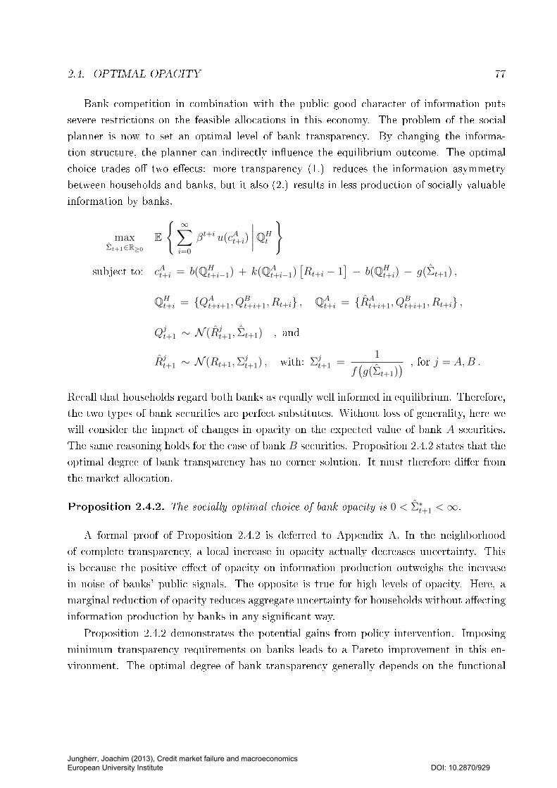
2.4. OPTIMAL OPACITY 77
Bank competition in combination with the public good character of information puts
severe restrictions on the feasible allocations in this economy. The problem of the social
planner is now to set an optimal level of bank transparency. By changing the informa-
tion structure, the planner can indirectly inuence the equilibrium outcome. The optimal
choice trades o two eects: more transparency (1.) reduces the information asymmetry
between households and banks, but it also (2.) results in less production of socially valuable
information by banks.
maxΣt+1∈R≥0
E
∞∑i=0
βt+i u(cAt+i)
∣∣∣∣QHt
subject to: cAt+i = b(QHt+i−1) + k(QA
t+i−1)[Rt+i − 1
]− b(QH
t+i) − g(Σt+1) ,
QHt+i = QA
t+i+1, QBt+i+1, Rt+i , QA
t+i = RAt+i+1, Q
Bt+i+1, Rt+i ,
Qjt+1 ∼ N (Rj
t+1, Σt+1) , and
Rjt+1 ∼ N (Rt+1,Σ
jt+1) , with: Σj
t+1 =1
f(g(Σt+1)
) , for j = A,B .
Recall that households regard both banks as equally well informed in equilibrium. Therefore,
the two types of bank securities are perfect substitutes. Without loss of generality, here we
will consider the impact of changes in opacity on the expected value of bank A securities.
The same reasoning holds for the case of bank B securities. Proposition 2.4.2 states that the
optimal degree of bank transparency has no corner solution. It must therefore dier from
the market allocation.
Proposition 2.4.2. The socially optimal choice of bank opacity is 0 < Σ∗t+1 <∞.
A formal proof of Proposition 2.4.2 is deferred to Appendix A. In the neighborhood
of complete transparency, a local increase in opacity actually decreases uncertainty. This
is because the positive eect of opacity on information production outweighs the increase
in noise of banks' public signals. The opposite is true for high levels of opacity. Here, a
marginal reduction of opacity reduces aggregate uncertainty for households without aecting
information production by banks in any signicant way.
Proposition 2.4.2 demonstrates the potential gains from policy intervention. Imposing
minimum transparency requirements on banks leads to a Pareto improvement in this en-
vironment. The optimal degree of bank transparency generally depends on the functional
Jungherr, Joachim (2013), Credit market failure and macroeconomics European University Institute
DOI: 10.2870/929
78 CHAPTER 2. BANK OPACITY
form of f(g) which determines the social value of costly information acquisition by banks.
If this function is very steep, then society has a lot to lose from reductions in information
expenditures by banks and the optimal level of bank transparency will be relatively low. The
same is true for high levels of fundamental uncertainty (σ2) and risk aversion, as these two
factors likewise increase the social benet of costly information acquisition. Note however
one interesting aspect of bank opacity in general: an increase in the degree of asymmetry of
information between households and banks may result in a welfare gain.
2.5 Discussion
We have seen that the private costs of public disclosure of banks' asset positions and risk
exposure are particularly high if proprietary information becomes public. The mechanism
described above applies to a wide range of credit decisions and asset classes. The problem of
opacity becomes particularly severe whenever (1.) bank competition is erce, and whenever
(2.) investment in information acquisition by banks can result in a considerable information
advantage.
Note that bank competition is part of the problem in this model and not part of the solu-
tion. The equilibrium allocation does not change qualitatively whether two banks compete
for households' savings or a large number of N banks. On the other hand, a monopolist
banker in a non-contestable market for nancial intermediation would be in a position to
reveal all available information to the public without the threat of adverse consequences
for her market share. The ineciencies with respect to the supply of public information
described above would cease to exist. However, other well-known ineciencies are bound to
arise in the presence of market power.
In the analysis above it is assumed that the information which banks choose to transmit
to the markets are veriable. In practice, banks report summary statistics of aggregated asset
positions and risk sensitivities estimated for selected scenarios. These reporting instruments
still leave some room for nancial window dressing. This may even be intended by regulation
as complete transparency is not desirable. On the other hand, information about asset
positions is socially valuable to the extent that the risk characteristics of the products held
by banks are understood by the public. If opacity results in a competitive advantage, then
we should expect banks to invest resources in the development of assets which are hard to
understand and to value for competitor banks. Cheng, Dhaliwal and Neamtiu (2008) nd
that empirically banks that engage in securitization transactions are more opaque than banks
with no asset securitizations.
Jungherr, Joachim (2013), Credit market failure and macroeconomics European University Institute
DOI: 10.2870/929
2.5. DISCUSSION 79
The review of the related literature has demonstrated that existing approaches to bank
transparency have found that not only the asset side of banks' balance sheet but also the
particularities of their liability structure yields interesting implications for the problem of
optimal bank transparency. The model outlined above is suciently general to encompass a
wide range of nancial intermediaries (e.g. mutual funds, hedge funds). Arguably, maturity
transformation is a central characteristic of banks and should be incorporated in the analysis
in order to study the impact of public disclosure on the stability of banks. After all, the
renewed interest in the topic of bank transparency has started with the recent crisis.
The introduction of a fragile liability structure could also shed new light on the related
topic of bank contagion. Jones, Lee and Yeager (2012) have demonstrated the tight empirical
link between informational opacity and bank contagion. Slovin, Sushka and Polonchek (1999)
show that informational contagion occurs more frequently among money center banks which
process large nancial ows through global networks, and less often among regional banks
which service a domestic-based clientele through branches and subsidiaries. This nding is
consistent with the notion that erce competition and information-intensive and complex
investment activities in the market of money center banks result in increased informational
opacity relative to less competitive regional banking markets, where eventual information
advantages are limited by the size of the market and the characteristics of available assets.
Jungherr, Joachim (2013), Credit market failure and macroeconomics European University Institute
DOI: 10.2870/929

80 CHAPTER 2. BANK OPACITY
Appendix A Proofs and Derivations
Proposition 2.3.3
Proof. The costs of a marginal investment in information acquisition must be equal to the
marginal benets in terms of a more protable and safer portfolio. The rst order condition
for a socially ecient choice of gAt+1 reads as:
∂
∂ gAt+1
[E ∞∑
i=0
βt+i u(c∗t+i)
∣∣∣∣Rt
]=
∂
∂ gAt+1
[EE ∞∑
i=0
βt+i u(c∗t+i)
∣∣∣∣ RAt+1, R
Bt+1, Rt
∣∣∣∣Rt
]= E
∂
∂ gAt+1
[E ∞∑
i=0
βt+i u(c∗t+i)
∣∣∣∣ RAt+1, R
Bt+1, Rt
] ∣∣∣∣Rt
= 0 .
For a given sample of observations Qt =RAt+1, R
Bt+1, Rt
, information expenditures must
pay o by making this information more reliable and thereby increasing its social value. Let
ϕ(Rt+1|RAt+1, R
Bt+1, Rt) denote the density of Rt+1 for a given sample of observations. Then
we can rewrite:
∂
∂ gAt+1
[E ∞∑
i=0
βt+i u(c∗t+i)
∣∣∣∣ RAt+1, R
Bt+1, Rt
]=
∂
∂ gAt+1
[ ∫ ( ∞∑i=0
βt+i u(c∗t+i)
)ϕ(Rt+1|RA
t+1, RBt+1, Rt) dRt+1
]=
∫ [∂
∂ gAt+1
( ∞∑i=0
βt+i u(c∗t+i)
)ϕ(Rt+1|RA
t+1, RBt+1, Rt)
+
( ∞∑i=0
βt+i u(c∗t+i)
)∂ ϕ(Rt+1|RA
t+1, RBt+1, Rt)
∂ gAt+1
]dRt+1
= E ∞∑
i=0
βt+i∂ u(c∗t+i)
∂ gAt+1
∣∣∣∣ RAt+1, R
Bt+1, Rt
+
∫ ( ∞∑i=0
βt+i u(c∗t+i)
)∂ ϕ(Rt+1|RA
t+1, RBt+1, Rt)
∂ gAt+1
dRt+1 .
The rst term of this sum captures the consequences of information expenditures in terms
of a reallocation of resources, while the second term measures the implied changes in the
Jungherr, Joachim (2013), Credit market failure and macroeconomics European University Institute
DOI: 10.2870/929

PROOFS AND DERIVATIONS 81
uncertainty regime which the planner has to face.
The envelope theorem allows us to abstract from indirect eects of changes in gAt+1 which
are transmitted through its impact on other choice variables. To see this, consider the welfare
eect of a change in b∗t+1 induced by the variation in gAt+1:
E ∞∑
i=0
βt+i∂ u(c∗t+i)
∂ b∗t+1
∂ b∗t+1
∂ gAt+1
∣∣∣∣ RAt+1, R
Bt+1, Rt
=∂ b∗t+1
∂ gAt+1
[− ∂ u(c∗t )
∂ c∗t+ β E
∂ u(c∗t+1)
∂ c∗t+1
∣∣∣∣ RAt+1, R
Bt+1, Rt
].
Note that the optimal choice of b∗t+1 =(RAt+1, R
Bt+1, Rt
)is dened by:
∂ u(c∗t )
∂ c∗t= β E
∂ u(c∗t+1)
∂ c∗t+1
∣∣∣∣ RAt+1, R
Bt+1, Rt
.
The same reasoning applies to indirect eects of changes in gAt+1 transmitted through other
choice variables, e.g. k∗t+1. It follows that:
E ∞∑
i=0
βt+i∂ u(c∗t+i)
∂ gAt+1
∣∣∣∣ RAt+1, R
Bt+1, Rt
= − β E
∂ u(c∗t+i)
∂ c∗t+1
∣∣∣∣ RAt+1, R
Bt+1, Rt
.
Increasing investment in information acquisition reduces the resources available at date t+1
for consumption. Now, the rst order condition for a socially ecient choice of gAt boils
down to:
β E∂ u(c∗t+1)
∂ c∗t+1
∣∣∣∣Rt
= E
∫ ( ∞∑i=0
βt+i u(c∗t+i)
)∂ ϕ(Rt+1|RA
t+1, RBt+1, Rt)
∂ gAt+1
dRt+1
∣∣∣∣Rt
.
The density of Rt+1 depends on gAt+1 through its conditional variance as given by:
VarRt+1
∣∣ RAt+1, R
Bt+1, Rt
=
σ2ΣAt+1ΣB
t+1
σ2ΣAt+1 + σ2ΣB
t+1 + ΣAt+1ΣB
t+1
.
Since we know that:
∂ VarRt+1
∣∣ RAt+1, R
Bt+1, Rt
∂ gAt+1
= −VarRt+1
∣∣ RAt+1, R
Bt+1, Rt
2f ′(gAt+1) ,
Jungherr, Joachim (2013), Credit market failure and macroeconomics European University Institute
DOI: 10.2870/929

82 CHAPTER 2. BANK OPACITY
we can rewrite the rst order condition for gAt according to:
β E∂ u(c∗t+1)
∂ c∗t+1
∣∣∣∣Rt
= E
∫ ( ∞∑i=0
βt+i u(c∗t+i)
)∂ ϕ(Rt+1|Qt)
∂ VarRt+1
∣∣Qt
∂ VarRt+1
∣∣Qt
∂ gAt+1
dRt+1
∣∣∣∣Rt
= −Var
Rt+1
∣∣Qt
2f ′(gAt+1) E
∫ ( ∞∑i=0
βt+i u(c∗t+i)
)∂ ϕ(Rt+1|Qt)
∂ VarRt+1
∣∣Qt
dRt+1
∣∣∣∣Rt
,
where Qt =RAt+1, R
Bt+1, Rt
. The function f(g) is increasing, strictly concave and satises
the Inada conditions, e.g. f ′(0) =∞ and f ′(∞) = 0. Furthermore, u(c) is strictly concave.
By Jensen's inequality, a mean preserving spread in the distribution of Rt+1 lowers expected
welfare. It follows that the right hand side of the equation above is strictly positive.
For gAt+1 = 0, the marginal benet of increasing information expenses on the right hand
side of the equation above exceeds the associated costs on the left hand side. As gAt+1 goes
towards innity, its marginal benets shrink while the marginal costs in terms of expected
welfare are growing without bounds. Only an interior choice of gA∗
t+1 can satisfy the rst order
condition. The analogue reasoning holds for the entirely symmetric problem of selecting
gB∗
t+1. Concavity of f(g) implies that the planner will optimally invest equal amounts in the
precision of both signals.
Proposition 2.3.5
Proof. In the neighborhood of the optimal level of gAt+1, a marginal adjustment must increase
households' valuation of bank A securities just as much as it increases the value of bank B
securities.
E
∂
∂ gAt+1
[E ∞∑
i=0
βt+i u(cAt+i)
∣∣∣∣ RAt+1, Rt
] ∣∣∣∣Rt
= E
∂
∂ gAt+1
[E ∞∑
i=0
βt+i u(cBt+i)
∣∣∣∣ RBt+1, Rt
] ∣∣∣∣Rt
.
Under complete opacity, the latter term is zero. The rst order condition for an optimal
choice of gAt+1 becomes:
E
∂
∂ gAt+1
[E ∞∑
i=0
βt+i u(cAt+i)
∣∣∣∣ RAt+1, Rt
] ∣∣∣∣Rt
= 0 .
Jungherr, Joachim (2013), Credit market failure and macroeconomics European University Institute
DOI: 10.2870/929

PROOFS AND DERIVATIONS 83
Applying the same reasoning as in the proof to Proposition 2.3.3 above, we can rewrite this
rst order condition according to:
β E∂ u(ct+1)
∂ ct+1
∣∣∣∣Rt
= E
∫ ( ∞∑i=0
βt+i u(cAt+i)
)∂ ϕ(Rt+1|RA
t+1, Rt)
∂ gAt+1
dRt+1
∣∣∣∣Rt
.
This is equivalent to:
β E∂ u(ct+1)
∂ ct+1
∣∣∣∣Rt
= −Var
Rt+1
∣∣QAt
2f ′(gAt+1) E
∫ ( ∞∑i=0
βt+i u(cAt+i)
)∂ ϕ(Rt+1|QA
t )
∂ VarRt+1
∣∣QAt
dRt+1
∣∣∣∣Rt
,
where QAt =
RAt+1, Rt
. Under opacity, bankers face a higher degree of uncertainty than
under transparency for given levels of information expenses:
VarRt+1
∣∣ RAt+1, Rt
=
σ2 ΣAt+1
σ2 + ΣAt+1
>
σ2ΣAt+1ΣB
t+1
σ2ΣAt+1 + σ2ΣB
t+1 + ΣAt+1ΣB
t+1
= VarRt+1
∣∣ RAt+1, R
Bt+1, Rt
.
Also, household welfare is reduced with respect to the case of exogenous transparency for
a given level of gAt+1. This is because both hoseholds' savings decisions as well as banks'
portfolio choice are based on less information now. Non-increasing absolute risk aversion
implies that given increases in uncertainty become more costly as expected consumption
levels fall. It follows that:
0 < gA∗
t+1 = gB∗
t+1 < gA∗∗
t+1 = gB∗∗
t+1 < ∞ .
Jungherr, Joachim (2013), Credit market failure and macroeconomics European University Institute
DOI: 10.2870/929
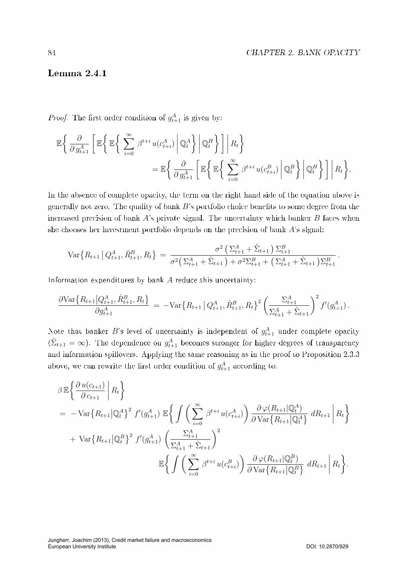
84 CHAPTER 2. BANK OPACITY
Lemma 2.4.1
Proof. The rst order condition of gAt+1 is given by:
E
∂
∂ gAt+1
[EE ∞∑
i=0
βt+i u(cAt+i)
∣∣∣∣QAt
∣∣∣∣QHt
] ∣∣∣∣Rt
= E
∂
∂ gAt+1
[EE ∞∑
i=0
βt+i u(cBt+i)
∣∣∣∣QBt
∣∣∣∣QHt
] ∣∣∣∣Rt
.
In the absence of complete opacity, the term on the right hand side of the equation above is
generally not zero. The quality of bank B's portfolio choice benets to some degree from the
increased precision of bank A's private signal. The uncertainty which banker B faces when
she chooses her investment portfolio depends on the precision of bank A's signal:
VarRt+1
∣∣QAt+1, R
Bt+1, Rt
=
σ2(
ΣAt+1 + Σt+1
)ΣBt+1
σ2(
ΣAt+1 + Σt+1
)+ σ2ΣB
t+1 +(
ΣAt+1 + Σt+1
)ΣBt+1
.
Information expenditures by bank A reduce this uncertainty:
∂VarRt+1
∣∣QAt+1, R
Bt+1, Rt
∂gAt+1
= −VarRt+1
∣∣QAt+1, R
Bt+1, Rt
2(
ΣAt+1
ΣAt+1 + Σt+1
)2
f ′(gAt+1) .
Note that banker B's level of uncertainty is independent of gAt+1 under complete opacity
(Σt+1 = ∞). The dependence on gAt+1 becomes stronger for higher degrees of transparency
and information spillovers. Applying the same reasoning as in the proof to Proposition 2.3.3
above, we can rewrite the rst order condition of gAt+1 according to:
β E∂ u(ct+1)
∂ ct+1
∣∣∣∣Rt
= −Var
Rt+1
∣∣QAt
2f ′(gAt+1) E
∫ ( ∞∑i=0
βt+i u(cAt+i)
)∂ ϕ(Rt+1|QA
t )
∂ VarRt+1
∣∣QAt
dRt+1
∣∣∣∣Rt
+ Var
Rt+1
∣∣QBt
2f ′(gAt+1)
(ΣAt+1
ΣAt+1 + Σt+1
)2
E∫ ( ∞∑
i=0
βt+i u(cBt+i)
)∂ ϕ(Rt+1|QB
t )
∂ VarRt+1
∣∣QBt
dRt+1
∣∣∣∣Rt
.
Jungherr, Joachim (2013), Credit market failure and macroeconomics European University Institute
DOI: 10.2870/929

PROOFS AND DERIVATIONS 85
In equilibrium, both banks spend identical amounts on information acquisition. Hence,
ex-ante their expected beliefs are identical:
Eϕ(Rt+1 |QA
t )
∣∣∣∣Rt
= E
ϕ(Rt+1 |QB
t )
∣∣∣∣Rt
.
Likewise, the symmetry of equilibrium implies:
VarRt+1
∣∣QAt
= Var
Rt+1
∣∣QBt
.
Hence, we can rewrite the rst order condition of gAt+1:
β E∂ u(ct+1)
∂ ct+1
∣∣∣∣Rt
= −Var
Rt+1
∣∣QAt
2f ′(gAt+1)
[1 −
(ΣAt+1
ΣAt+1 + Σt+1
)2 ]E ∫ ( ∞∑
i=0
βt+iu(cAt+i)
)∂ ϕ(Rt+1|QA
t )
∂ VarRt+1
∣∣QAt
dRt+1
∣∣∣∣Rt
.
Under complete transparency (Σt+1 = 0), the right hand side of this equation is always zero
and so is the optimal choice of gAt+1. As Σt+1 is growing, the rival bank participates less and
less in improvements to bank A's information set.
Note that:
limΣt+1→∞
∂
∂ Σt+1
[(ΣAt+1
ΣAt+1 + Σt+1
)2 ]= lim
Σt+1→∞
[− 2
ΣAt+1
2(ΣAt+1 + Σt+1
)3
]= 0 ,
and also:
limΣt+1→∞
∂
∂ Σt+1
[VarRt+1
∣∣QAt
]= lim
Σt+1→∞
[(VarRt+1
∣∣QAt
ΣAt+1 + Σt+1
)2 ]= 0 .
For high values of opacity, the signal-to-noise ratio of banks' public signals becomes less and
less responsive to additional changes in opacity. This is reected by the vanishing dependence
of the optimal choice of gAt+1 on the degree of information spillovers:
limΣt+1→∞
g′(Σt+1) = 0 .
Jungherr, Joachim (2013), Credit market failure and macroeconomics European University Institute
DOI: 10.2870/929

86 CHAPTER 2. BANK OPACITY
Proposition 2.4.2
Proof. The rst order condition for a socially optimal choice of Σt+1 is given by:
∂
∂ Σt+1
[EE ∞∑
i=0
βt+i u(cAt+i)
∣∣∣∣QAt
∣∣∣∣QHt
]= 0 .
A change in opacity has two eects on welfare: (1.) uncertainty for households varies with
the informational content of QHt = QA
t+1, QBt+1, Rt, and (2.) the uncertainty for banks is
aected through QAt = RA
t+1, QBt+1, Rt. This can be seen from rewriting:
∂
∂ Σt+1
[EE ∞∑
i=0
βt+i u(cAt+i)
∣∣∣∣QAt
∣∣∣∣QHt
]=
∂
∂ Σt+1
[ ∫E ∞∑
i=0
βt+i u(cAt+i)
∣∣∣∣QAt
ϕ(Rt+1|QH
t ) dRt+1
].
From the product rule, it follows that:
∂
∂ Σt+1
[ ∫E ∞∑
i=0
βt+i u(cAt+i)
∣∣∣∣QAt
ϕ(Rt+1|QH
t ) dRt+1
]=
∫∂
∂ Σt+1
[E ∞∑
i=0
βt+i u(cAt+i)
∣∣∣∣QAt
]ϕ(Rt+1|QH
t ) dRt+1
+
∫E ∞∑
i=0
βt+i u(cAt+i)
∣∣∣∣QAt
∂ ϕ(Rt+1|QH
t )
∂ Σt+1
dRt+1
= E
∂
∂ Σt+1
[E ∞∑
i=0
βt+i u(cAt+i)
∣∣∣∣QAt
] ∣∣∣∣QHt
+
∫E ∞∑
i=0
βt+i u(cAt+i)
∣∣∣∣QAt
∂ ϕ(Rt+1|QH
t )
∂ Σt+1
dRt+1 .
The rst term of this sum captures households' expectations about how the change in opacity
will aect the precision of bank A's forecast of Rt+1:
E
∂
∂ Σt+1
[E ∞∑
i=0
βt+i u(cAt+i)
∣∣∣∣QAt
] ∣∣∣∣QHt
= E
∫ ( ∞∑i=0
βt+iu(cAt+i)
)∂ ϕ(Rt+1|QA
t )
∂ Σt+1
dRt+1
∣∣∣∣QHt
.
Jungherr, Joachim (2013), Credit market failure and macroeconomics European University Institute
DOI: 10.2870/929
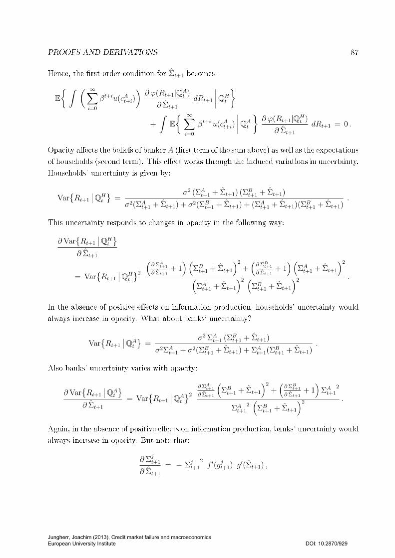
PROOFS AND DERIVATIONS 87
Hence, the rst order condition for Σt+1 becomes:
E ∫ ( ∞∑
i=0
βt+iu(cAt+i)
)∂ ϕ(Rt+1|QA
t )
∂ Σt+1
dRt+1
∣∣∣∣QHt
+
∫E ∞∑
i=0
βt+i u(cAt+i)
∣∣∣∣QAt
∂ ϕ(Rt+1|QH
t )
∂ Σt+1
dRt+1 = 0 .
Opacity aects the beliefs of bankerA (rst term of the sum above) as well as the expectations
of households (second term). This eect works through the induced variations in uncertainty.
Households' uncertainty is given by:
VarRt+1
∣∣QHt
=
σ2 (ΣAt+1 + Σt+1) (ΣB
t+1 + Σt+1)
σ2(ΣAt+1 + Σt+1) + σ2(ΣB
t+1 + Σt+1) + (ΣAt+1 + Σt+1)(ΣB
t+1 + Σt+1).
This uncertainty responds to changes in opacity in the following way:
∂ VarRt+1
∣∣QHt
∂ Σt+1
= VarRt+1
∣∣QHt
2
(∂ ΣAt+1
∂ Σt+1+ 1)(
ΣBt+1 + Σt+1
)2
+(∂ ΣBt+1
∂ Σt+1+ 1)(
ΣAt+1 + Σt+1
)2
(ΣAt+1 + Σt+1
)2 (ΣBt+1 + Σt+1
)2 .
In the absence of positive eects on information production, households' uncertainty would
always increase in opacity. What about banks' uncertainty?
VarRt+1
∣∣QAt
=
σ2 ΣAt+1 (ΣB
t+1 + Σt+1)
σ2ΣAt+1 + σ2(ΣB
t+1 + Σt+1) + ΣAt+1(ΣB
t+1 + Σt+1).
Also banks' uncertainty varies with opacity:
∂ VarRt+1
∣∣QAt
∂ Σt+1
= VarRt+1
∣∣QAt
2
∂ ΣAt+1
∂ Σt+1
(ΣBt+1 + Σt+1
)2
+(∂ ΣBt+1
∂ Σt+1+ 1)
ΣAt+1
2
ΣAt+1
2(
ΣBt+1 + Σt+1
)2 .
Again, in the absence of positive eects on information production, banks' uncertainty would
always increase in opacity. But note that:
∂ Σjt+1
∂ Σt+1
= − Σjt+1
2f ′(gjt+1) g′(Σt+1) ,
Jungherr, Joachim (2013), Credit market failure and macroeconomics European University Institute
DOI: 10.2870/929

88 CHAPTER 2. BANK OPACITY
which is always negative. By Lemma 2.4.1, this term converges to zero as opacity tends
towards innity. At Σt+1 = 0, its value is −∞. Information production is highly responsive
for low levels of opacity. This sensitivity falls as opacity is increased.
This implies for the uncertainty of households and bankers, respectively:
∂ VarRt+1
∣∣QHt
∂ Σt+1
< 0 , and∂ Var
Rt+1
∣∣QAt
∂ Σt+1
< 0 , for Σt+1 = 0 .
In the neighborhood of complete transparency, a local increase in opacity actually decreases
uncertainty. This is because the positive eect of opacity on information production out-
weighs the increase in noise of banks' public signals. The opposite is true for high levels of
opacity:
∂ VarRt+1
∣∣QHt
∂ Σt+1
> 0 , and∂ Var
Rt+1
∣∣QAt
∂ Σt+1
> 0 , for Σt+1 =∞ .
In the neighborhood of complete opacity, a marginal reduction of opacity reduces aggre-
gate uncertainty for households without aecting information production by banks in any
signicant way. Reconsider now the rst order condition of Σt+1:
∂VarRt+1
∣∣QAt
∂Σt+1
E∫ ( ∞∑
i=0
βt+iu(cAt+i)
)∂ϕ(Rt+1|QA
t )
∂VarRt+1
∣∣QAt
dRt+1
∣∣∣∣QHt
+∂Var
Rt+1
∣∣QHt
∂Σt+1
∫E ∞∑
i=0
βt+i u(cAt+i)
∣∣∣∣QAt
∂ϕ(Rt+1|QH
t )
∂VarRt+1
∣∣QHt
dRt+1 = 0 .
It becomes clear that the social benets of increasing opacity are positive at Σt+1 = 0. The
opposite is true for Σt+1 =∞.
Jungherr, Joachim (2013), Credit market failure and macroeconomics European University Institute
DOI: 10.2870/929
BIBLIOGRAPHY 89
Bibliography
Admati, Anat R. and Paul Peiderer (1988). `Selling and Trading on Information in Financial Markets,'The American Economic Review, Vol. 78(2), pp. 96-103.
Admati, Anat R. and Paul Peiderer (1990). `Direct and Indirect Sale of Information,' Econometrica, Vol.58(4), pp. 901-928.
Admati, Anat R. and Paul Peiderer (2000). `Forcing Firms to Talk: Financial Disclosure Regulation andExternalities,' The Review of Financial Studies, Vol. 13(3), pp. 479-519.
Alvarez, Fernando and Gadi Barlevy (2013). `Mandatory Disclosure and Financial Contagion,' mimeo, July2013.
Bernanke, Ben S. (2010). `Remarks on The Squam Lake Report: Fixing the Financial System,' Remarksat the Squam Lake Conference, New York, New York, U.S., June 16, 2010.
Blackwell, David (1951). `Comparison of Experiments,' in: Jerzy Neyman (ed.), Proceedings of the Second
Berkeley Symposium on Mathematical Statistics and Probability. July 31-August 12, 1950. Statistical Labo-
ratory of the University of California, Berkeley, pp. 93-102, University of California Press, Berkeley.
Bouvard, Matthieu, Pierre Chaigneau, and Adolfo de Motta (2012). `Transparency in the Financial System:Rollover Risk and Crises,' mimeo, August 2012.
Chen, Yehning and Iftekhar Hasan (2006). `The Transparency of the Banking System and the Eciency ofInformation-Based Bank Runs,' Journal of Financial Intermediation, Vol. 15, pp. 307-331.
Cheng, Mei, Dan Dhaliwal and Monica Neamtiu (2008). `Banks' Asset Securitization and Information Opac-ity,' mimeo, April 2008.
Dang, Tri Vi, Gary Gorton, Bengt Holmström, and Guillermo Ordoñez (2013). `Banks as Secret Keepers,'mimeo, May 2013.
Darrough, Masako N. and Neal M. Stoughton (1990). `Financial Disclosure Policy in an Entry Game,' Jour-nal of Accounting and Economics, Vol. 12, pp. 219-243.
Diamond, Douglas D. (1985). `Optimal Release of Information of Firms,' The Journal of Finance, Vol. 40(4),pp. 1071-1094.
Dye, Ronald A. (1986). `Proprietary and Nonproprietary Disclosures,' The Journal of Business, Vol. 59(2),pp. 331-366.
Dye, Ronald A. (1990). `Mandatory versus Voluntary Disclosures: The Cases of Financial and Real Exter-nalities,' The Accounting Review, Vol. 65(1), pp. 1-24.
Flannery, Mark J., Simon H. Kwan, and M. Nimalendran (2004). `Market Evidence on the Opaqueness ofBanking Firms' Assets,' Journal of Financial Economics, Vol. 71, pp. 419-460.
Foster, George (1980). `Externalities and Financial Reporting,' The Journal of Finance, Vol. 35(2), pp.521-533.
French, K., M. Baily, J. Campbell, J. Cochrane, D. Diamond, D. Due, A. Kashyap, F. Mishkin, R. Rajan,D. Scharfstein, R. Shiller, H. Shin, M. Slaughter, J. Stein, and R. Stulz (2010). The Squam Lake Report:
Fixing the Financial System, Princeton University Press, Princeton and Oxford.
Goldstein, Itay and Haresh Sapra (2012). `Should Banks' Stress Test Results be Disclosed? An Analysis ofthe Costs and Benets,' mimeo, April 2012.
Jungherr, Joachim (2013), Credit market failure and macroeconomics European University Institute
DOI: 10.2870/929
90 CHAPTER 2. BANK OPACITY
Grossman, Sanford J. and Oliver D. Hart (1980). `Disclosure Laws and Takeover Bids,' The Journal of
Finance, Vol. 35(2), pp. 323-334.
Grossman, Sanford J. and Joseph E. Stiglitz (1976). `Information and Competitive Price Systems,' TheAmerican Economic Review, Vol. 66(2), pp. 246-253.
Grossman, Sanford J. and Joseph E. Stiglitz (1980). `On the Impossibility of Informationally Ecient Mar-kets,' The American Economic Review, Vol. 70(3), pp. 393-408.
Hirshleifer, Jack (1971). `The Private and Social Value of Information and the Reward to Inventive Activity,'The American Economic Review, Vol. 61(4), pp. 561-574.
Hirtle, Beverly (2006). `Stock Market Reaction to Financial Statement Certication by Bank Holding Com-pany CEOs,' Journal of Money, Credit and Banking, Vol. 38(5), pp. 1263-1291.
Iannotta, Giuliano (2006). `Testing for Opaqueness in the European Banking Industry: Evidence from BondCredit Ratings,' Journal of Financial Services Research, Vol. 30, pp. 287-309.
Jones, Jerey S., Wayne Y. Lee, and Timothy J. Yeager (2012). `Opaque Banks, Price Discovery, and Fi-nancial Instability,' Journal of Financial Intermediation, Vol. 21, pp. 383-408.
Kurlat, Pablo and Laura Veldkamp (2012). `Should We Regulate Financial Information?' mimeo, May 2012.
Landier, Augustin and David Thesmar (2011). `Regulating Systemic Risk through Transparency: Tradeosin Making Data Public,' in: Markus K. Brunnermeier and Arvind Krishnamurthy (ed.), Risk Topography:
Systemic Risk and Macro Modeling, forthcoming from University of Chicago Press, Chicago.
Marschak, Jacob (1955). `Elements for a Theory of Teams,' Management Science, Vol. 1(2), pp. 127-137.
Moreno, Diego and Tuomas Takalo (2012). `Optimal Bank Transparency,' mimeo, November 2012.
Morgan, Donald P. (2002). `Rating Banks: Risk and Uncertainty in an Opaque Industry,' The American
Economic Review, Vol. 92(4), pp. 874-888.
Morris, Stephen and Hyun Song Shin (2002). `Social Value of Public Information,' The American Economic
Review, Vol. 92(5), pp. 1521-1534.
Pagano, Marco and Paolo Volpin (2012). `Securitization, Transparency, and Liquidity,' The Review of Fi-
nancial Studies, Vol. 25(8), pp. 2417-2453.
Radner, Roy (1962). `Team Decision Problems,' The Annals of Mathematical Statistics, Vol. 33(3), pp.857-881.
Slovin, Myron B., Marie E. Sushka and John A. Polonchek (1999). `An Analysis of Contagion and Compet-itive Eects at Commercial Banks,' Journal of Financial Economics, Vol. 54(2), pp. 197-225.
Spargoli, Fabrizio (2012). `Bank's Optimal Information Disclosure and Banks' Opacity,' mimeo, October2012.
Verrecchia, Robert E. (1983). `Discretionary Disclosure,' Journal of Accounting and Economics, Vol. 5, pp.179-194.
Vives, Xavier (2012), `Endogenous Public Information and Welfare,' IESE Working Paper No. 925, April2012.
Jungherr, Joachim (2013), Credit market failure and macroeconomics European University Institute
DOI: 10.2870/929
Chapter 3
Why Does Misallocation Persist?
with David Strauss (European University Institute)
3.1 Introduction
Why are some countries so rich while others are poor? Hsieh and Klenow (2010) calculate
that 10-30 percent of cross-country income dierences can be explained by dierent levels
of human capital, while about 20 percent are attributable to dierences in physical capital.
The most important part of 50-70 percent is accounted for by dierences in total factor
productivity (TFP) across countries. But why do TFP levels dier so vastly across countries?
The recent growth literature has identied the misallocation of production factors within
countries as a potentially powerful explanation device for large TFP dierences.1 In search
for a reason for severe factor misallocation, capital market imperfections have been a popular
subject of inquiry.2 However, the quantitative eect on TFP of factor misallocation caused by
credit market frictions can be quite disappointing.3 One important reason for this negative
result is that borrowing constraints are only a temporary obstacle for capital accumulation
if self-nancing is possible.4
1See Banerjee and Duo (2005), Guner, Ventura and Xu (2008), Restuccia and Rogerson (2008), Hsiehand Klenow (2009), or Bartelsman, Haltiwanger and Scarpetta (2013). An early study of the role of factormisallocation for TFP is Hopenhayn and Rogerson (1993).
2The role of factor misallocation caused by credit market frictions for growth and development has recentlybeen explored by Giné and Townsend (2004), Jeong and Townsend (2007), Greenwood, Sanchez and Wang(2010), Buera, Kaboski and Shin (2011), Moll (2012), Buera and Shin (2013), Caselli and Gennaioli (2013),Greenwood, Sanchez and Wang (2013), and others.
3See Hosono and Takizawa (2012), Gilchrist, Sim and Zakraj²ek (2013), and Midrigan and Xu (2013).4This point has been made by Banerjee and Moll (2010) and Moll (2012).
91
Jungherr, Joachim (2013), Credit market failure and macroeconomics European University Institute
DOI: 10.2870/929
92 CHAPTER 3. PERSISTENT MISALLOCATION
We contribute to this literature by proposing a model in which factor misallocation
caused by capital market imperfections may indeed give rise to permanent income and TFP
dierences across countries. In the presence of binding credit constraints, the assignment of
human capital to heterogeneous production sectors is completely reversed with respect to the
case of ecient capital markets. This misallocation of skill across sectors may be permanent
because the model features a collective poverty trap which arises for low levels of nancial
development. This poverty trap is the result of a pecuniary externality which rm owners
inict on workers by selecting the sector of production. Depending on initial conditions,
a country converges over time to one of two dierent stable steady states characterized by
dierent long-run levels of output, capital, wages, and measured TFP.
The comparison of these two stable long-run equilibria yields additional interesting re-
sults. First, manufactured goods are relatively cheaper in a country which has reached the
high-income steady state compared to a country which has converged to the low-income equi-
librium. This corresponds well with the empirical results of Parente and Prescott (2002) and
Hsieh and Klenow (2007) who nd that manufactured goods are relatively more expensive in
nancially underdeveloped economies. Furthermore, both the average rm size in terms of
capital as well as its variance are higher in the high-income steady state. Hopenhayn (2012)
reports that the rm-size distributions of India and Mexico, as measured by the number of
employees, are compressed with respect to the U.S. (but also with respect to China) once
average rm size is controlled for.
Preview of the Model
At the core of the model lies a static assignment problem. There are two production sectors:
manufacturing and services. Production takes place in many rms. Each of them uses
a single worker and some quantity of capital as input factors. The manufacturing sector
is more capital-intensive than services, as the input productivity of capital is higher in
manufacturing. Workers dier according to their human capital (or talent). Workers of high
ability reduce the failure rate of production and they also produce more than low ability
workers in case production succeeds. Manufactured goods and service goods are aggregated
to the numéraire good which is a simple Cobb-Douglas composite of the two intermediate
goods. Firm owners choose to produce one of the two intermediate goods depending on the
ability of their randomly drawn worker. This assignment problem of workers of dierent
quality to production sectors of dierent capital eciency is embedded in a highly stylized
overlapping generations model. Young agents work and save in order to become a rm owner
once they are too old to work themselves. In addition to their own savings, rm owners have
Jungherr, Joachim (2013), Credit market failure and macroeconomics European University Institute
DOI: 10.2870/929
3.1. INTRODUCTION 93
access to the international capital market at an exogenous interest rate.
Results
The key result of the paper is the central importance of nancial development for the growth
trajectory and the convergence properties of the model economy. A low level of nancial
development is characterized by tight credit constraints for domestic rm owners who are
seeking to obtain capital on the international credit market.5 First, we show that the equilib-
rium assignment of human capital to production sectors of dierent capital input productivity
is completely reversed in the presence of binding borrowing constraints with respect to the
case of ecient capital markets. This formal result conrms a conjecture by Sampson (2011).
Assume that worker talent is a close substitute for capital productivity in the production
function. In this case, labor quality and capital productivity are also gross substitutes in
rm earnings as long as capital is exogenously xed. However, under increasing returns
to worker talent, capital productivity and labor quality become gross complements in rm
earnings once capital is set optimally. As the matching of human capital to production
sectors depends on the degree of complementarity between the attributes of workers and
sectors, an assignment reversal occurs.
We go on to show that this assignment reversal gives rise to the possibility of multiple
stable steady states. Depending on the initial domestic stock of capital, the model economy
converges to one of two dierent long-run equilibria which are characterized by dierent
sorting patterns and consequently also dierent levels of measured TFP, wages, capital,
and per capita income. The reason for the possibility of multiple steady states is that an
assignment reversal causes a discrete upward jump in a country's level of measured TFP.
But rm owners need to be able to produce on a suciently large scale before it becomes
protable for rms with workers of dierent quality to switch production sectors. Financially
underdeveloped countries may reach a low-income and low-capital steady state before the
sorting reversal occurs. In this case, the misallocation of human capital to production sectors
is permanent.
Self-nancing provides an imperfect substitute for functioning credit markets. If a coun-
try starts with a suciently high level of domestic capital, it may converge to a second
steady state which is characterized by an ecient sorting pattern of workers into production
sectors, and consequently also high levels of measured TFP, wages, capital, and per capita
5Borrowing constraints may arise in equilibrium in the presence of limited contract enforceability. In thiscase, the upper limit for credit is falling in the share of borrowed funds which can be diverted by debtors,while it rises with the pledgeable fraction of rm owners' private wealth.
Jungherr, Joachim (2013), Credit market failure and macroeconomics European University Institute
DOI: 10.2870/929

94 CHAPTER 3. PERSISTENT MISALLOCATION
income. This high-income steady state may be reached even under nancial autarky, if initial
conditions are suciently favorable.
The allocation of human capital across production sectors is ecient in the high-income
steady state. If worker ability and capital enter the production function as gross substitutes,
then it is ecient for high talent agents to produce capital-intensive manufacturing goods
since they are the ones who benet most from large scales of production. A given quantity
of manufactured goods can be produced at a lower cost by high talent workers than by low
ability agents. Consequently, manufacturing goods are relatively cheaper in the high-income
equilibrium.
Also the rm size distribution diers across steady states depending on the respective
sorting pattern. Even if not all rm owners are credit constrained in the low-income equilib-
rium, the rm size distribution will still be compressed as high talent workers are employed
in the sector with low capital productivity and vice versa. This reduces the benets of lever-
aging workers' talent through capital. In contrast, in the high-income steady state it is the
high ability workers which produce in the sector in which capital is used most eciently.
Consequently, the incentives to combine high talent with a large amount of capital are much
higher now. The opposite is true for low ability workers who produce using a technology
characterized by low capital productivity. Therefore, both the average rm size and its
variance are higher in the high-income steady state than in the low-income equilibrium.
Related Literature
Our paper starts from the observation that quantitative models of credit market imper-
fections have diculties to generate permanent and sizeable TFP dierences through pure
factor misallocation. Using U.S. data on rm-specic borrowing costs, Gilchrist, Sim and
Zakraj²ek (2013) nd large and persistent dierences in borrowing costs across rms on the
corporate bond market. However, in their model these dierences in nancing conditions
do not translate into large TFP losses due to resource misallocation. Hosono and Takizawa
(2012) estimate only a slightly higher impact of borrowing constraints on factor misallocation
and aggregate TFP in japanese plant-level data.
While these two studies analyze data from highly developed economies, Midrigan and Xu
(2013) compare South Korea as a country with a well developed nancial sector with China
and Colombia as examples for nancially underdeveloped economies. The authors nd a
strong eect of borrowing constraints on entry and technology adoption, but only a weak
impact on pure factor misallocation across establishments. The reason for this negative
result is that credit constraints are only a temporary obstacle for capital accumulation if
Jungherr, Joachim (2013), Credit market failure and macroeconomics European University Institute
DOI: 10.2870/929
3.1. INTRODUCTION 95
self-nancing is possible. In the data, rm productivity is suciently persistent in order to
allow productive establishments to simply grow out of their nancial constraints.
These ndings are in contrast to the large TFP losses attributed to credit market fric-
tions by other studies. These contributions tend to rely on the extensive margin of factor
misallocation. Giné and Townsend (2004) and Jeong and Townsend (2007) study the high
growth period in Thailand 1976-1996. They nd that exogenous nancial deepening allowed
productive agents to leave the subsistence sector and become entrepreneurs. Similarly, also
in Erosa and Cabrillana (2008), Amaral and Quintin (2010), and Greenwood, Sanchez and
Wang (2013), it is an exogenous improvement in the eciency of the nancial intermediation
sector which results in the usage of more ecient production technologies. Caselli and Gen-
naioli (2013) focus on dynastic management of family-owned rms, which can be a source
of the mismatch between talent and wealth. The demographic structure of these studies (or
the modeling of rms as short-term projects) excludes or severely restricts the possibility of
self-nancing. This is a key reason for the important role of nancial development in these
models. If agents (or rms) were allowed to accumulate wealth over time, then this would
provide a substitute for credit markets and could result in a minor role of nancial frictions
for long-run factor misallocation.6
Note that this criticism does not apply to our model. In the studies cited above, dif-
ferences in nancial development are a sucient condition for dierences in TFP across
countries. In our OLG framework, binding borrowing constraints are merely a necessary
condition for permanent TFP dierences between countries. It is possible that in both
steady states at least some rm owners are credit constrained. Still, in one of these steady
states the allocation of human capital across plants is ecient while in the other steady state
it is not. In the absence of a poverty trap, the model economy would grow over time until
the allocation of worker talent is fully ecient. It is in this sense that we contribute to the
literature by introducing a new mechanism that allows for permanent TFP losses through
factor misallocation caused by credit market frictions.7
Pursuing a similar research question to ours, Buera, Kaboski and Shin (2011) examine
the eect of credit constraints on the allocation of entrepreneurial talent and capital across
manufacturing and services. The authors explicitly show the role of the self-nancing channel
in mitigating the adverse consequences of credit constraints by comparing the quantitative
results of a model featuring long-lived agents with an OLG setup. But even allowing for
6For a formal discussion of the self-nancing channel, see also Banerjee and Moll (2010) and Moll (2012).7Of course, within an OLG framework it is impossible to fully address the concerns arising from the
self-nancing channel. It is an important open question whether the described poverty trap can exist alsoin a model populated by long-lived agents. See also Section 3.5 for a short discussion of future work.
Jungherr, Joachim (2013), Credit market failure and macroeconomics European University Institute
DOI: 10.2870/929
96 CHAPTER 3. PERSISTENT MISALLOCATION
the possibility of self-nancing, they still nd that nancial frictions can account for TFP
losses of up to 40 percent. Non-convexities in production play a key role. Also, the authors
use a less persistent productivity process for individual entrepreneurs than Midrigan and
Xu (2013). Moll (2012) argues that the magnitude of TFP losses is highly sensitive to the
exact value of persistence in productivity processes. Large and permanent TFP losses do not
seem to be a robust result in existing models of factor misallocation through credit market
frictions. Buera and Shin (2013) focus on the role of nancial frictions in delaying the speed
of convergence towards a stationary equilibrium. They nd that self-nancing is only an
imperfect substitute for functioning credit markets as transition takes roughly twice as long
as in the neoclassical growth model. In contrast to our paper, both Buera, Kaboski and Shin
(2011) and Buera and Shin (2013) feature a unique stationary equilibrium.
Obviously, we are not the rst to show how credit market imperfections may give rise
to multiple stable equilibria along the growth path of an economy. Banerjee and Newman
(1993) discuss the central importance of the income distribution for the development process
of a country. If a lot of agents are rich enough to become entrepreneurs, this results in
high wages for poor workers in their model which in turn allows a lot of agents to start
their own business in the future. A more skewed initial income distribution results in less
entrepreneurial activity and lower wages in the long run. Buera (2008) shows that this
multiplicity result survives in an environment where self-nancing is possible. Also in Galor
and Zeira (1993), credit market frictions result in a pecuniary externality which current
generations inict on their ospring. Similarly to Banerjee and Newman (1993), the income
distribution is a state variable in their model which features multiple steady states. Both in
Banerjee and Newman (1993) as well as in Galor and Zeira (1993), agents are homogeneous
and TFP in a given production sector is always constant across dierent equilibria. In our
model, TFP within a given sector diers across equilibria. This is an important result in
light of the empirical evidence on sector-specic productivity dierences across countries
provided by Erosa and Cabrillana (2008) or Buera, Kaboski and Shin (2011).8
Our work also relates to the literature on equilibrium matching. We build on Sampson
(2011) who describes the conditions under which log-submodularity in production translates
into log-supermodularity in earnings and vice versa.9 He also provides empirical evidence on
sorting reversals across countries. In the data, the assignment of human capital to production
8Examples of poverty traps which do not aect technological choice or factor misallocation can be foundin Piketty (1997), Ghatak, Morelli and Sjöström (2001), or Mookerjee and Ray (2002).
9Complementarity has been identied as the decisive factor in driving ecient matching since the classiccontribution by Becker (1973). See also Costinot (2009) for a denition and discussion of log-supermodularityand log-submodularity.
Jungherr, Joachim (2013), Credit market failure and macroeconomics European University Institute
DOI: 10.2870/929
3.1. INTRODUCTION 97
sectors seems to depend crucially on the respective state of economic development. The
model by Sampson (2011) features assignment reversals across countries because of exogenous
dierences in the ranking of sectors according to capital input productivity. In our setting,
the sorting pattern of worker talent into heterogeneous production sectors depends on a
country's domestic stock of capital. If rms are able to set capital optimally, the matching
pattern reverses with respect to the case of binding borrowing constraints.
Also Legros and Newman (2002) point out that imperfect credit markets may distort the
equilibrium sorting pattern associated with a frictionless environment. In some cases, this
may even result in an assignment reversal. In contrast to our model, Legros and Newman
(2002) assume non-convexities in production. In their model, assignment reversals may or
may not arise in the presence of nancial frictions depending on the underlying distribution of
types, while in our model sorting reversals are a necessary consequence of binding borrowing
constraints.
Poverty traps arise in our model only for low levels of nancial development. This cen-
tral role of nancial development for growth has been established by numerous empirical
studies. King and Levine (1993) and Levine and Zervos (1998) estimate a close link between
aggregate measures of credit and nancial development across countries on the one hand
and output per capita on the other hand. Further evidence is provided using sector-level
data (Rajan and Zingales, 1998) and rm-level data (Beck, Demirgüç-Kunt and Maksimovic,
2005) across countries. Importantly, Beck, Levine and Loayza (2000) nd that the positive
impact of nancial development on economc growth is transmitted through TFP growth.
Also the results by La Porta, Lopez-de-Silanes, Shleifer and Vishny (1998) on institutional
dierences such as contract enforcement and creditor protection support the idea that nan-
cial development is tightly linked to economic growth. Banerjee and Duo (2005) review
micro-level evidence for credit constraints in poor countries and the resulting misallocation
of capital.
Outline
The rest of the paper is organized as follows. The model is set up in Section 3.2. Section
3.3 characterizes the ecient allocation of production factors across sectors. In Section 3.4,
the implications of credit constraints for static and dynamic ineciencies are discussed. The
paper concludes with a short discussion of potential enhancements of the model in Section
3.5.
Jungherr, Joachim (2013), Credit market failure and macroeconomics European University Institute
DOI: 10.2870/929

98 CHAPTER 3. PERSISTENT MISALLOCATION
3.2 Model Setup
Consider an overlapping generations model. Each agent lives for two periods and each
generation has unit mass. When agents are young, they are endowed with their ability as
workers and their working time. Workers are heterogeneous with respect to their talent.
During their youth, they can save their wages in order to become rm owners once they
are too old to work. A rm owner can choose to produce one of two intermediate goods:
manufacturing or services. The manufacturing sector is more capital-intensive than the
service sector. These intermediate goods are used in the production of the numéraire good
which can be consumed or sold on the international goods market.
3.2.1 Agents
All agents in this model economy are risk averse and they consume only when they are old.
There is no disutility of work and therefore each young agent supplies in equilibrium her full
working time endowment l = 1 on the labor market. A young agent's preferences at time t
can be described by the function:
Et u(ct+1) ,
where Et is the expectation operator conditional on date t information. The function u :
R≥0 → R satises the Inada conditions. Young agents use their wage wt to buy capital at
the end of their youth:
wt = kt+1 .
Old agents employ this capital kt+1 in a rm. Production is risky and all agents are risk
averse. Hence, old agents will optimally insure each other against their idiosyncratic risks.
Old agents consume all of their wealth. Accordingly, the budget constraint of an old agent
z ∈ [0, 1] reads as:
ct+1(z) ≤ Πt+1(z) + Tt+1(z) ,
where Πt+1(z) gives the rm prots of agent z's rm and Tt+1(z) denotes the insurance
payment which is conditional on the production outcome. This insurance transfer can be
positive or negative.
3.2.2 Production
A rm owner has access to two dierent production technologies: manufacturing or services.
In both cases, output is produced using capital and a single worker as inputs. Workers dier
Jungherr, Joachim (2013), Credit market failure and macroeconomics European University Institute
DOI: 10.2870/929
3.2. MODEL SETUP 99
with respect to their talent. A fraction ϕ of workers has a high ability θ = θH and a mass
1 − ϕ of young agents has a low level of talent: θ = θL, with θH > θL. The output yjt+1(z)
of an old agent z's rm in sector j = m, s is given by:
yjt+1(z) =
F(θ(z), QjKt+1(z)
),with probability π
(θ(z)
), and
0 , otherwise.
The production function F : R≥0 × R≥0 → R≥0 has constant returns to scale and is dened
over the hired worker's talent θ and capital Kt+1. The function is increasing and strictly
concave in both arguments with: F2(θ, 0) = ∞ and F2(θ,∞) = 0. The manufacturing
sector is more ecient in using capital: Qm > Qs. Production is risky as a rm owner
faces each period a probability of 1− π(θ) that output is zero. The success probability π(θ)
is strictly increasing in the worker's talent. Note that this implies that expected output
features increasing returns to scale.10
Firm owner z ∈ [0, 1] decides conditional on the talent of her worker θ(z) whether to
produce in sector m or in sector s. She also has the option to rent capital dt+1(z) on an
international capital market at a rate of r in order to lever up rm prots. These prots are
given by:
Πt+1(z) = pjt+1 yjt+1(z) − wt+1 − (1 + r)Kt+1(z) ,
where: Kt+1(z) = kt+1(z) + dt+1(z).
3.2.3 Final Good
Manufacturing and service goods are used in the production of the numéraire good which
can be consumed or sold on the international goods market. This nal good is produced
using a Cobb-Douglas technology according to:
yt+1 =(ymt+1
)αm (yst+1
)αs,
10The function of expected output is similar to the output of a manager-worker pair in Rosen (1982) whostudies a single sector model of rm hierarchies. In Rosen (1982), increasing returns to managerial skill arisedue to the scale-independent importance of managerial decisions for all other factors of production. In ourmodel, it is the talent-dependent success probability which introduces increasing returns to worker ability.
Jungherr, Joachim (2013), Credit market failure and macroeconomics European University Institute
DOI: 10.2870/929

100 CHAPTER 3. PERSISTENT MISALLOCATION
where αm + αs = 1. There are no additional costs in the production of this nal good and
the nal goods sector is perfectly competitive:
yt+1 = pmt+1 ymt+1 + pst+1 y
st+1 .
The nal goods producers make exactly zero prots in each period.
3.2.4 Labor Market
A young agent supplies her labor force on the period t labor market. An agent can only work
for a single rm and every rm owner can hire only one worker. For the sake of tractability,
we assume that both rm owners and workers learn the ability of a worker only after the
labor contract is signed. Therefore, all workers on the labor market are ex-ante identical and
there is a homogeneous wage rate wt for all worker-rm owner pairs. As workers sell their
labor in one piece and not at the margin, the division of the surplus between workers and
rm owners depends on the bargaining weight γ ∈ (0, 1) of workers. The outside option of
workers is zero, while the outside option of rm owners is the international capital market.
3.2.5 Timing
At time t, young agents are born with an endowment of working time and some level of
talent θ. Old agents enter the period with a predetermined stock of savings kt. They insure
themselves against their idiosyncratic risks of production. The labor market opens and old
agents hire workers at a wage rate wt. After they learn the talent of their worker, each
rm owner now decides in which sector to produce and how much capital dt to rent on the
international capital market. Production takes place and the intermediate goods are bought
by the nal goods producers which subsequently oer the nal good on the consumption
goods market. Old agents consume their wealth and young agents use their wages to buy
capital goods for period t+ 1.
3.3 Ecient Allocation
Before studying the implications of credit constraints for the misallocation of production
factors in this model economy, we take a look at a frictionless world where capital markets
work smoothly and the allocation of resources is perfectly ecient.
Jungherr, Joachim (2013), Credit market failure and macroeconomics European University Institute
DOI: 10.2870/929
3.3. EFFICIENT ALLOCATION 101
Denition Given some initial capital stock of old agents kt and the rental rate r on the
international capital market, a competitive equilibrium in this economy consists of an as-
signment function j∗(θ, kt+i), a production policy K∗(θ, j, kt+i), prices w∗t+i, p
mt+i, p
st+i, and a
capital stock k∗t+i+1, such that (1.) young agents save their wages, (2.) old agents solve their
individual optimization problem by choosing j∗(θ, kt+i) and K∗(θ, j, kt+i), (3.) the labor
market clears, and (4.) the intermediate goods market clears.
3.3.1 Production
Consider rst the problem of rm owner z ∈ [0, 1] at time t who has drawn a worker of talent
θ on the labor market and who has chosen to produce in sector j. Firm owners optimally
insure each other against the idiosyncratic risk of production failure as well as the risk of
ending up with a worker of low talent. The law of large numbers holds and the optimal
insurance transfer makes sure that each rm owner in this model economy receives the ex-
ante expected level of rm output with certainty. Firm owners have to decide on the optimal
scale of production. Expected prots conditional on the worker's talent θ and the production
sector j are maximized according to:
maxKt ∈ [0,+∞)
π(θ)pjt F
(θ, QjKt
)− wt − (1 + r) [Kt − kt ] . (3.1)
Constant returns to scale allow us to express production in terms of a single variable:
f
(QjKt
θ
)≡ 1
θF(θ, QjKt
).
The optimal scale of production satises the following rst order condition:
π(θ)pjt Q
j f ′(QjK∗(θ, j, kt)
θ
)= (1 + r) .
The expected marginal product of capital must be equal to its costs. This can be rewritten
according to:
f ′(QjK∗(θ, j, kt)
θ
)=
1 + r
π(θ)pjt Q
j. (3.2)
Jungherr, Joachim (2013), Credit market failure and macroeconomics European University Institute
DOI: 10.2870/929
102 CHAPTER 3. PERSISTENT MISALLOCATION
We have expressed the optimal scale of production in terms of a single variable. This variable
is the span of control of a worker:
σjt (θ) ≡QjKt
θ.
The span of control measures the eciency units of capital used at time t per unit of talent
and captures the extent to which a rm chooses to leverage the ability of its worker by
contracting capital. As the function f : R≥0 → R≥0 is strictly concave, it follows from the
rst order condition in (3.2) that σjt (θ) is optimally increasing in the worker's talent θ, the
intermediate good's price pjt , and input productivity Qj.11
3.3.2 Sorting
After rm owners learn the talent of their randomly assigned worker, they select their pre-
ferred production sector anticipating the respective optimal capital policy K∗(θ, j, kt) as
described by (3.2). Both intermediate goods are necessary in order to produce a positive
quantity of the nal good. Therefore, some rm owners should choose to produce the man-
ufactured good while others must sort into the services industry. It is not possible that
intermediate goods markets clear if all rm owners strictly prefer one sector of production
over the other.
Firm owners dier according to their worker's ability. The two sectors of production
dier according to their eciency in using capital as an input factor. The manufacturing
sector's technology strictly dominates services in terms of eciency. If rm owners with
high talent workers strictly prefer the manufacturing sector and/or if rm owners with low
talent workers strictly prefer the service sector over manufacturing, then we will have positive
assortative matching (PAM). In this case, it holds that:
π(θH)pmt θH f
(QmK∗(θH ,m, kt)
θH
)− wt − (1 + r)
[K∗(θH ,m, kt)− kt
]≥ π
(θH)pst θ
H f
(QsK∗(θH , s, kt)
θH
)− wt − (1 + r)
[K∗(θH , s, kt)− kt
],
11Production per unit of worker talent features diminishing returns to the span of control as in Lucas(1978). If a worker is using more machines, she has less time for each single unit and marginal returns arefalling in scale.
Jungherr, Joachim (2013), Credit market failure and macroeconomics European University Institute
DOI: 10.2870/929

3.3. EFFICIENT ALLOCATION 103
and:
π(θL)pmt θL f
(QmK∗(θL,m, kt)
θL
)− wt − (1 + r)
[K∗(θL,m, kt)− kt
]≤ π
(θL)pst θ
L f
(QsK∗(θL, s, kt)
θL
)− wt − (1 + r)
[K∗(θL, s, kt)− kt
],
with at least one of the two inequalities above being strict. The opposite case is negative
assortative matching (NAM). In any case, intermediate good prices adjust in a way such
that the optimal span of control of a worker of given talent is higher in manufacturing than
in services as shown by Lemma 3.3.1.
Lemma 3.3.1. In equilibrium, it must hold that: σmt∗(θ) > σst
∗(θ).
Proof. Taking as given the intermediate goods prices and using:
K∗(θ, j, kt) =θ σjt
∗(θ)
Qj,
as well as the rst order condition in (3.2), we can rewrite rm prots according to:
Πjt
∗(θ) = pjt π
(θ)θ[f(σjt∗(θ))− σjt
∗(θ) f ′
(σjt∗(θ)) ]− wt + (1 + r) kt .
The term in square brackets is strictly increasing in the optimal span of control:
∂
∂ σjt∗(θ)
[f(σjt∗(θ))− σjt
∗(θ) f ′
(σjt∗(θ)) ]
= − σjt∗(θ) f ′′
(σjt∗(θ)).
Since by equation (3.2) the optimal span of control is strictly increasing in pjtQjt , it follows
that also the term above is strictly increasing in pjtQjt .
Assume now for a moment that manufacturing goods are more expensive than service
goods: pmt > pst . Then it also holds that: pmt Qmt > pstQ
st . But in this case Πm
t∗(θ) > Πm
t∗(θ)
for all rm owners and nobody chooses to produce service goods. This is incompatible with
intermediate goods markets clearing. It follows that in equilibrium: pmt < pst .
Since pmt < pst , it follows in turn that pmt Qmt > pstQ
st in equilibrium. Otherwise, nobody
chooses to produce manufactured goods. From (3.2), it follows then that for a worker of
given talent the optimal span of control is strictly higher in manufacturing than in the
service sector.
No matter which level of talent the workers in manufacturing possess, rm owners will
Jungherr, Joachim (2013), Credit market failure and macroeconomics European University Institute
DOI: 10.2870/929

104 CHAPTER 3. PERSISTENT MISALLOCATION
optimally lever up their abilities using a higher span of control than rm owners in the
service sector do. Firm output per unit of worker ability responds to an increase in the span
of control according to the point elasticity of f(σt(θ)
):
εf(σt(θ)
)≡
f ′(σt(θ)
)σt(θ)
f(σt(θ)
) .
This elasticity diers across sectors together with the optimal span of control. In any given
sector, the optimal span of control is higher if high talent workers are employed. Proposition
3.3.2 shows that the ecient assignment of human capital to production sectors crucially
depends on the output elasticity dened above.
Proposition 3.3.2. Given well functioning credit markets, the equilibrium is characterized
by positive assortative matching (PAM) if the output elasticity εf(σt(θ)
)is strictly increasing
in the span of control. Negative assortative matching (NAM) arises if εf(σt(θ)
)is strictly
decreasing. Sorting is undertermined if εf(σt(θ)
)is constant.
Proof. Consider again the conditions for PAM as dened above. Taking as given intermediate
goods prices, we can rewrite this condition applying the same reasoning as in the proof of
Lemma 3.3.1:
f(σmt∗(θH)
)− σmt
∗(θH) f ′(σmt∗(θH)
)f(σst∗(θH)
)− σst
∗(θH) f ′(σst∗(θH)
) >f(σmt∗(θL)
)− σmt
∗(θL) f ′(σmt∗(θL)
)f(σst∗(θL)
)− σst
∗(θL) f ′(σst∗(θL)
) .
Rewriting this ratio across sectors using (3.2):
f(σmt∗(θ)
)− σmt
∗(θ) f ′(σmt∗(θ)
)f(σst∗(θ)
)− σst
∗(θ) f ′(σst∗(θ)
) =f(σmt∗(θ)
)− σmt
∗(θ) (1+r)
π(θ) pmt Qm
f(σst∗(θ)
)− σst
∗(θ) (1+r)
π(θ) pst Qs
,
and taking its derivative with respect to θ yields:
∂
∂θ
f(σmt ∗(θ)) − σmt∗(θ) (1+r)
π(θ) pmt Qm
f(σst∗(θ)
)− σst
∗(θ) (1+r)
π(θ) pst Qs
∝ f
(σmt∗(θ)
) [π(θ) f
(σst∗(θ)
)− σst
∗(θ) (1 + r)
pst Qs
]− f
(σst∗(θ)
) [π(θ) f
(σmt∗(θ)
)− σmt
∗(θ) (1 + r)
pmt Qm
].
Jungherr, Joachim (2013), Credit market failure and macroeconomics European University Institute
DOI: 10.2870/929
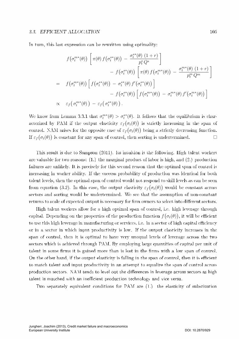
3.3. EFFICIENT ALLOCATION 105
In turn, this last expression can be rewritten using optimality:
f(σmt∗(θ)
) [π(θ) f
(σst∗(θ)
)− σst
∗(θ) (1 + r)
pst Qs
]− f
(σst∗(θ)
) [π(θ) f
(σmt∗(θ)
)− σmt
∗(θ) (1 + r)
pmt Qm
]= f
(σmt∗(θ)
) [f(σst∗(θ)
)− σst
∗(θ) f ′(σst∗(θ)
) ]− f
(σst∗(θ)
) [f(σmt∗(θ)
)− σmt
∗(θ) f ′(σmt∗(θ)
) ]∝ εf
(σmt∗(θ)
)− εf
(σst∗(θ)
).
We know from Lemma 3.3.1 that σmt∗(θ) > σst
∗(θ). It follows that the equilibrium is char-
acterized by PAM if the output elasticity εf(σt(θ)
)is strictly increasing in the span of
control. NAM arises for the opposite case of εf(σt(θ)
)being a strictly decreasing function.
If εf(σt(θ)
)is constant for any span of control, then sorting is undertermined.
This result is due to Sampson (2011). Its intuition is the following. High talent workers
are valuable for two reasons: (1.) the marginal product of labor is high, and (2.) production
failures are unlikely. It is precisely for this second reason that the optimal span of control is
increasing in worker ability. If the success probability of production was identical for both
talent levels, then the optimal span of control would not respond to skill levels as can be seen
from equation (3.2). In this case, the output elasticity εf(σt(θ)
)would be constant across
sectors and sorting would be undertermined. We see that the assumption of non-constant
returns to scale of expected output is necessary for rm owners to select into dierent sectors.
High talent workers allow for a high optimal span of control, i.e. high leverage through
capital. Depending on the properties of the production function f(σt(θ)
), it will be ecient
to use this high leverage in manufacturing or services, i.e. in a sector of high capital eciency
or in a sector in which input productivity is low. If the output elasticity increases in the
span of control, then it is optimal to have very unequal levels of leverage across the two
sectors which is achieved through PAM. By employing large quantities of capital per unit of
talent in some rms it is gained more than is lost in the rms with a low span of control.
On the other hand, if the output elasticity is falling in the span of control, then it is ecient
to match talent and input productivity in an attempt to equalize the span of control across
production sectors. NAM tends to level out the dierences in leverage across sectors as high
talent is matched with an inecient production technology and vice versa.
Two separately equivalent conditions for PAM are (1.) the elasticity of substitution
Jungherr, Joachim (2013), Credit market failure and macroeconomics European University Institute
DOI: 10.2870/929
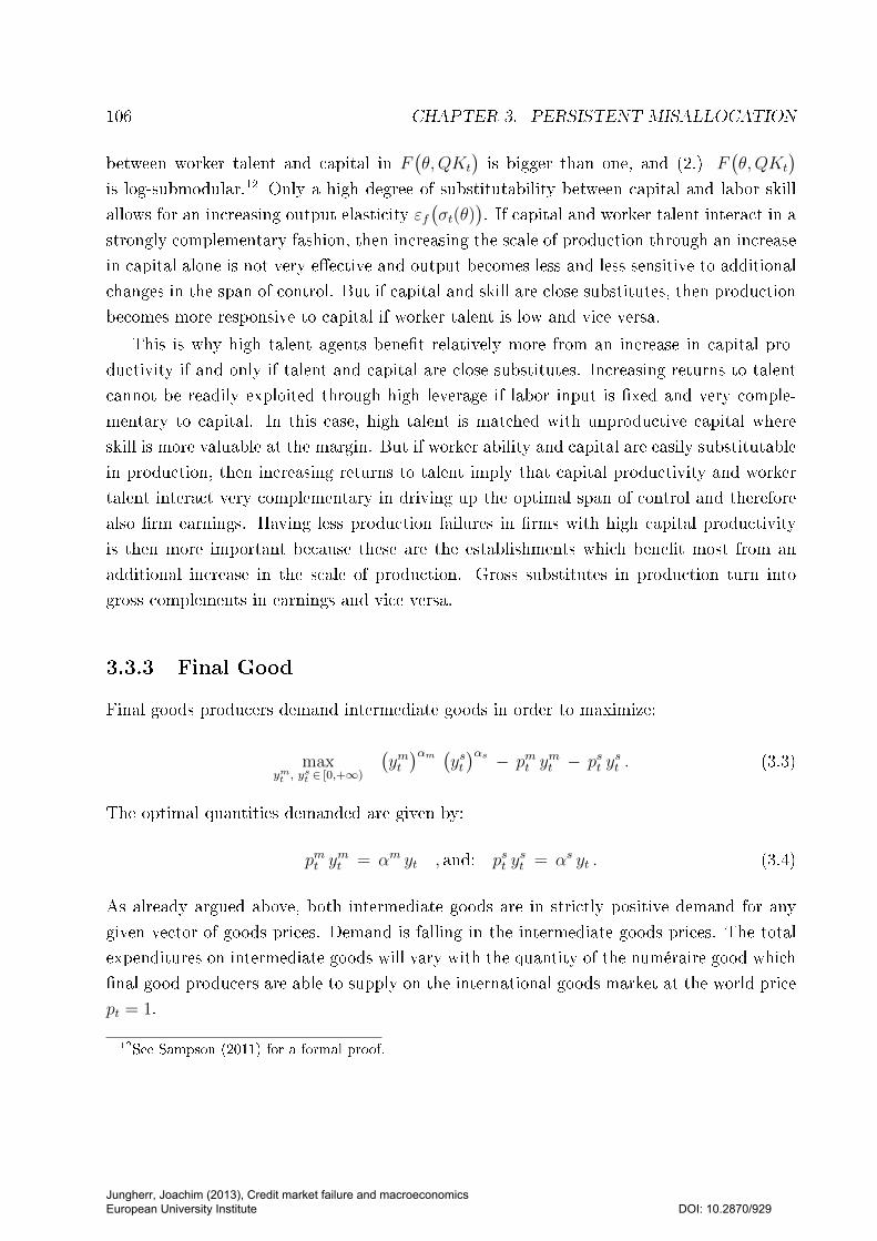
106 CHAPTER 3. PERSISTENT MISALLOCATION
between worker talent and capital in F(θ,QKt
)is bigger than one, and (2.) F
(θ,QKt
)is log-submodular.12 Only a high degree of substitutability between capital and labor skill
allows for an increasing output elasticity εf(σt(θ)
). If capital and worker talent interact in a
strongly complementary fashion, then increasing the scale of production through an increase
in capital alone is not very eective and output becomes less and less sensitive to additional
changes in the span of control. But if capital and skill are close substitutes, then production
becomes more responsive to capital if worker talent is low and vice versa.
This is why high talent agents benet relatively more from an increase in capital pro-
ductivity if and only if talent and capital are close substitutes. Increasing returns to talent
cannot be readily exploited through high leverage if labor input is xed and very comple-
mentary to capital. In this case, high talent is matched with unproductive capital where
skill is more valuable at the margin. But if worker ability and capital are easily substitutable
in production, then increasing returns to talent imply that capital productivity and worker
talent interact very complementary in driving up the optimal span of control and therefore
also rm earnings. Having less production failures in rms with high capital productivity
is then more important because these are the establishments which benet most from an
additional increase in the scale of production. Gross substitutes in production turn into
gross complements in earnings and vice versa.
3.3.3 Final Good
Final goods producers demand intermediate goods in order to maximize:
maxymt , y
st ∈ [0,+∞)
(ymt)αm (
yst)αs − pmt y
mt − pst y
st . (3.3)
The optimal quantities demanded are given by:
pmt ymt = αm yt , and: pst y
st = αs yt . (3.4)
As already argued above, both intermediate goods are in strictly positive demand for any
given vector of goods prices. Demand is falling in the intermediate goods prices. The total
expenditures on intermediate goods will vary with the quantity of the numéraire good which
nal good producers are able to supply on the international goods market at the world price
pt = 1.
12See Sampson (2011) for a formal proof.
Jungherr, Joachim (2013), Credit market failure and macroeconomics European University Institute
DOI: 10.2870/929
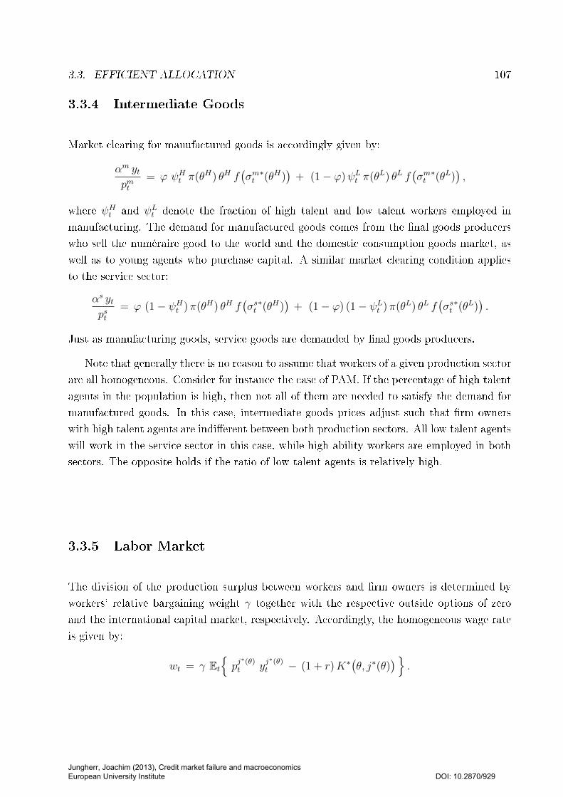
3.3. EFFICIENT ALLOCATION 107
3.3.4 Intermediate Goods
Market clearing for manufactured goods is accordingly given by:
αm ytpmt
= ϕ ψHt π(θH) θH f(σmt∗(θH)
)+ (1− ϕ)ψLt π(θL) θL f
(σmt∗(θL)
),
where ψHt and ψLt denote the fraction of high talent and low talent workers employed in
manufacturing. The demand for manufactured goods comes from the nal goods producers
who sell the numéraire good to the world and the domestic consumption goods market, as
well as to young agents who purchase capital. A similar market clearing condition applies
to the service sector:
αs ytpst
= ϕ (1− ψHt )π(θH) θH f(σst∗(θH)
)+ (1− ϕ) (1− ψLt ) π(θL) θL f
(σst∗(θL)
).
Just as manufacturing goods, service goods are demanded by nal goods producers.
Note that generally there is no reason to assume that workers of a given production sector
are all homogeneous. Consider for instance the case of PAM. If the percentage of high talent
agents in the population is high, then not all of them are needed to satisfy the demand for
manufactured goods. In this case, intermediate goods prices adjust such that rm owners
with high talent agents are indierent between both production sectors. All low talent agents
will work in the service sector in this case, while high ability workers are employed in both
sectors. The opposite holds if the ratio of low talent agents is relatively high.
3.3.5 Labor Market
The division of the production surplus between workers and rm owners is determined by
workers' relative bargaining weight γ together with the respective outside options of zero
and the international capital market, respectively. Accordingly, the homogeneous wage rate
is given by:
wt = γ Etpj∗(θ)t y
j∗(θ)t − (1 + r)K∗
(θ, j∗(θ)
).
Jungherr, Joachim (2013), Credit market failure and macroeconomics European University Institute
DOI: 10.2870/929
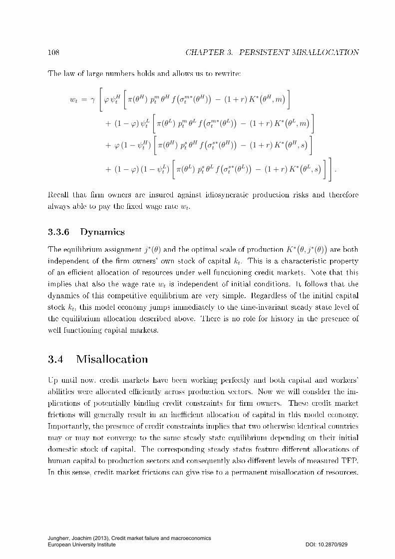
108 CHAPTER 3. PERSISTENT MISALLOCATION
The law of large numbers holds and allows us to rewrite:
wt = γ
[ϕψHt
[π(θH) pmt θ
H f(σmt∗(θH)
)− (1 + r)K∗
(θH ,m
) ]+ (1− ϕ)ψLt
[π(θL) pmt θ
L f(σmt∗(θL)
)− (1 + r)K∗
(θL,m
) ]+ ϕ (1− ψHt )
[π(θH) pst θ
H f(σst∗(θH)
)− (1 + r)K∗
(θH , s
) ]+ (1− ϕ) (1− ψLt )
[π(θL) pst θ
L f(σst∗(θL)
)− (1 + r)K∗
(θL, s
) ] ].
Recall that rm owners are insured against idiosyncratic production risks and therefore
always able to pay the xed wage rate wt.
3.3.6 Dynamics
The equilibrium assignment j∗(θ) and the optimal scale of production K∗(θ, j∗(θ)
)are both
independent of the rm owners' own stock of capital kt. This is a characteristic property
of an ecient allocation of resources under well functioning credit markets. Note that this
implies that also the wage rate wt is independent of initial conditions. It follows that the
dynamics of this competitive equilibrium are very simple. Regardless of the initial capital
stock kt, this model economy jumps immediately to the time-invariant steady state level of
the equilibrium allocation described above. There is no role for history in the presence of
well functioning capital markets.
3.4 Misallocation
Up until now, credit markets have been working perfectly and both capital and workers'
abilities were allocated eciently across production sectors. Now we will consider the im-
plications of potentially binding credit constraints for rm owners. These credit market
frictions will generally result in an inecient allocation of capital in this model economy.
Importantly, the presence of credit constraints implies that two otherwise identical countries
may or may not converge to the same steady state equilibrium depending on their initial
domestic stock of capital. The corresponding steady states feature dierent allocations of
human capital to production sectors and consequently also dierent levels of measured TFP.
In this sense, credit market frictions can give rise to a permanent misallocation of resources.
Jungherr, Joachim (2013), Credit market failure and macroeconomics European University Institute
DOI: 10.2870/929

3.4. MISALLOCATION 109
With respect to the previous section, the economic environment is modied by the following
assumption:
(A1) Credit Constraint. There is a maximum amount which a rm owner can borrow
on the international capital market: dt ≤ d.
The borrowing constraint d may be a function of rm owner's private wealth, the world
interest rate r or other variables. In the following, we will merely assume that d is always
identical for all rm owners in both production sectors and that the constraint is binding
given the initial domestic stock of capital kt.13
3.4.1 Production
Revisit the problem of a rm owner who has drawn a worker of talent θ on the labor market
and who has chosen to produce in sector j. Firm owners face a binding borrowing constraint
on the international capital market: dt ≤ d. This implies:
π(θ)pjt Q
j f ′
(Qj[kt + d
]θ
)> (1 + r) .
The optimal span of control associated with the ecient allocation is bigger for high ability
workers. Once capital is not set optimally anymore, this is no longer the case. The span of
control is still increasing in the capital productivity parameter Qj, but for a given production
sector the span of control is now higher for low talent workers than for high ability agents!
3.4.2 Sorting
How does this change in the environment aect the sorting pattern in this model economy?
The amount of borrowed capital is now identical across production sectors. The necessary
and sucient condition for PAM can be simplied to:
f(Qm[kt+d]
θH
)f(Qs[kt+d]
θH
) >f(Qm[kt+d]
θL
)f(Qs[kt+d]
θL
) .13We do not explicitly model the particular market failure which gives to this credit constraint in equilib-
rium. Limited contract enforceability on the capital market is one possibility. Note that we maintain ourassumption of perfect insurance among rm owners.
Jungherr, Joachim (2013), Credit market failure and macroeconomics European University Institute
DOI: 10.2870/929
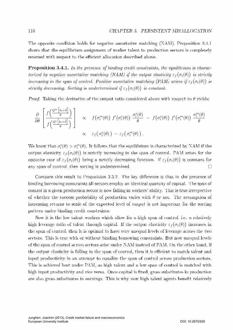
110 CHAPTER 3. PERSISTENT MISALLOCATION
The opposite condition holds for negative assortative matching (NAM). Proposition 3.4.1
shows that the equilibrium assignment of worker talent to production sectors is completely
reversed with respect to the ecient allocation described above.
Proposition 3.4.1. In the presence of binding credit constraints, the equilibrium is charac-
terized by negative assortative matching (NAM) if the output elasticity εf(σt(θ)
)is strictly
increasing in the span of control. Positive assortative matching (PAM) arises if εf(σt(θ)
)is
strictly decreasing. Sorting is undertermined if εf(σt(θ)
)is constant.
Proof. Taking the derivative of the output ratio considered above with respect to θ yields:
∂
∂θ
f(Qm[kt+d]
θ
)f(Qs[kt+d]
θ
) ∝ f
(σmt (θ)
)f ′(σst (θ)
) σst (θ)θ
− f(σst (θ)
)f ′(σmt (θ)
) σmt (θ)
θ
∝ εf(σst (θ)
)− εf
(σmt (θ)
).
We know that σst (θ) > σmt (θ). It follows that the equilibrium is characterized by NAM if the
output elasticity εf(σt(θ)
)is strictly increasing in the span of control. PAM arises for the
opposite case of εf(σt(θ)
)being a strictly decreasing function. If εf
(σt(θ)
)is constant for
any span of control, then sorting is undertermined.
Compare this result to Proposition 3.3.2. The key dierence is that in the presence of
binding borrowing constraints all sectors employ an identical quantity of capital. The span of
control in a given production sector is now falling in workers' ability. This is true irrespective
of whether the success probability of production varies with θ or not. The assumption of
increasing returns to scale of the expected level of output is not important for the sorting
pattern under binding credit constraints.
Now it is the low talent workers which allow for a high span of control, i.e. a relatively
high leverage ratio of talent through capital. If the output elasticity εf(σt(θ)
)increases in
the span of control, then it is optimal to have very unequal levels of leverage across the two
sectors. This is true with or without binding borrowing constraints. But now unequal levels
of the span of control across sectors arise under NAM instead of PAM. On the other hand, if
the output elasticity is falling in the span of control, then it is ecient to match talent and
input productivity in an attempt to equalize the span of control across production sectors.
This is achieved best under PAM, as high talent and a low span of control is matched with
high input productivity and vice versa. Once capital is xed, gross substitutes in production
are also gross substitutes in earnings. This is why now high talent agents benet relatively
Jungherr, Joachim (2013), Credit market failure and macroeconomics European University Institute
DOI: 10.2870/929
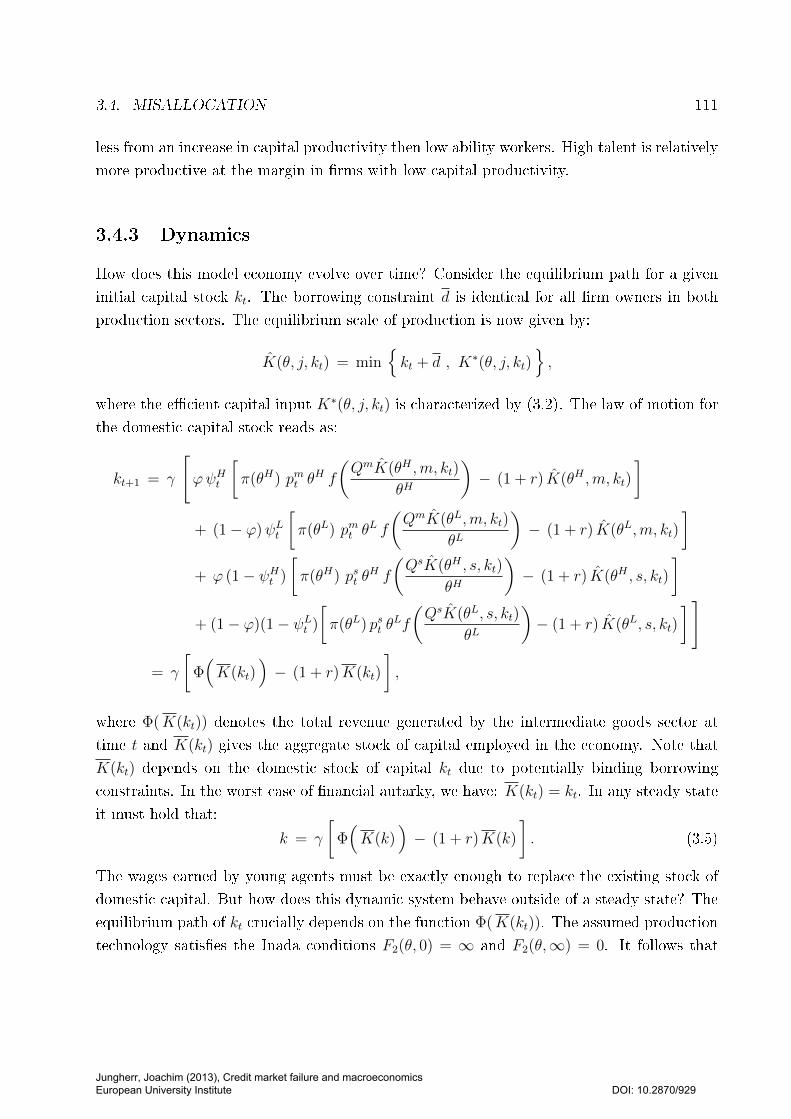
3.4. MISALLOCATION 111
less from an increase in capital productivity then low ability workers. High talent is relatively
more productive at the margin in rms with low capital productivity.
3.4.3 Dynamics
How does this model economy evolve over time? Consider the equilibrium path for a given
initial capital stock kt. The borrowing constraint d is identical for all rm owners in both
production sectors. The equilibrium scale of production is now given by:
K(θ, j, kt) = minkt + d , K∗(θ, j, kt)
,
where the ecient capital input K∗(θ, j, kt) is characterized by (3.2). The law of motion for
the domestic capital stock reads as:
kt+1 = γ
[ϕψHt
[π(θH) pmt θ
H f
(QmK(θH ,m, kt)
θH
)− (1 + r) K(θH ,m, kt)
]+ (1− ϕ)ψLt
[π(θL) pmt θ
L f
(QmK(θL,m, kt)
θL
)− (1 + r) K(θL,m, kt)
]+ ϕ (1− ψHt )
[π(θH) pst θ
H f
(QsK(θH , s, kt)
θH
)− (1 + r) K(θH , s, kt)
]+ (1− ϕ)(1− ψLt )
[π(θL) pst θ
Lf
(QsK(θL, s, kt)
θL
)− (1 + r) K(θL, s, kt)
]]
= γ
[Φ(K(kt)
)− (1 + r)K(kt)
],
where Φ(K(kt)) denotes the total revenue generated by the intermediate goods sector at
time t and K(kt) gives the aggregate stock of capital employed in the economy. Note that
K(kt) depends on the domestic stock of capital kt due to potentially binding borrowing
constraints. In the worst case of nancial autarky, we have: K(kt) = kt. In any steady state
it must hold that:
k = γ
[Φ(K(k)
)− (1 + r)K(k)
]. (3.5)
The wages earned by young agents must be exactly enough to replace the existing stock of
domestic capital. But how does this dynamic system behave outside of a steady state? The
equilibrium path of kt crucially depends on the function Φ(K(kt)). The assumed production
technology satises the Inada conditions F2(θ, 0) = ∞ and F2(θ,∞) = 0. It follows that
Jungherr, Joachim (2013), Credit market failure and macroeconomics European University Institute
DOI: 10.2870/929
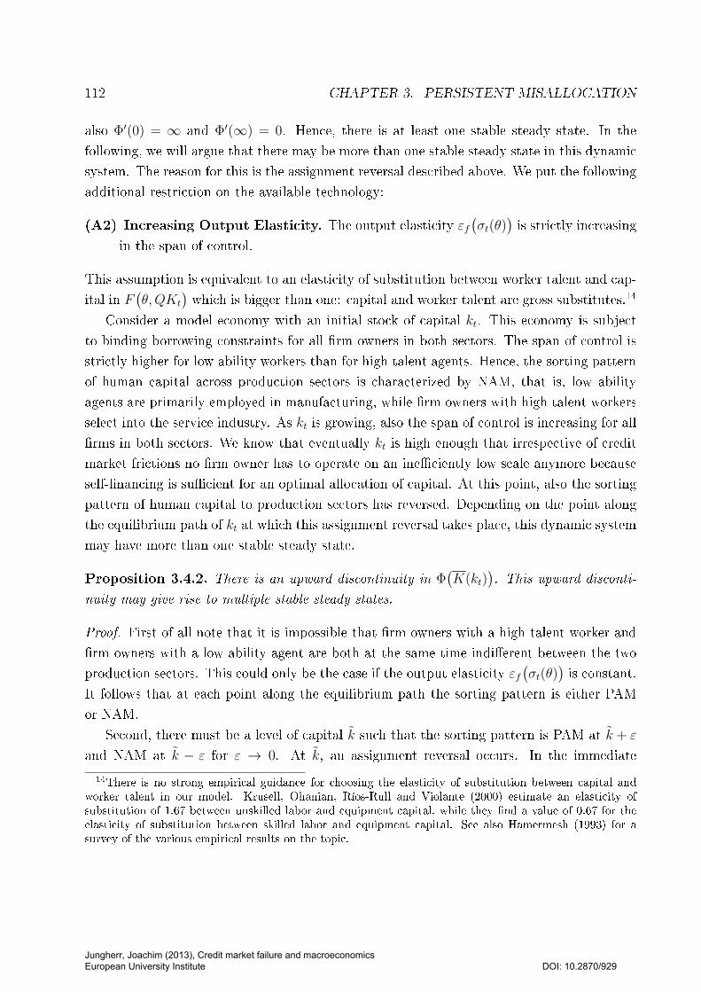
112 CHAPTER 3. PERSISTENT MISALLOCATION
also Φ′(0) = ∞ and Φ′(∞) = 0. Hence, there is at least one stable steady state. In the
following, we will argue that there may be more than one stable steady state in this dynamic
system. The reason for this is the assignment reversal described above. We put the following
additional restriction on the available technology:
(A2) Increasing Output Elasticity. The output elasticity εf(σt(θ)
)is strictly increasing
in the span of control.
This assumption is equivalent to an elasticity of substitution between worker talent and cap-
ital in F(θ,QKt
)which is bigger than one: capital and worker talent are gross substitutes.14
Consider a model economy with an initial stock of capital kt. This economy is subject
to binding borrowing constraints for all rm owners in both sectors. The span of control is
strictly higher for low ability workers than for high talent agents. Hence, the sorting pattern
of human capital across production sectors is characterized by NAM, that is, low ability
agents are primarily employed in manufacturing, while rm owners with high talent workers
select into the service industry. As kt is growing, also the span of control is increasing for all
rms in both sectors. We know that eventually kt is high enough that irrespective of credit
market frictions no rm owner has to operate on an ineciently low scale anymore because
self-nancing is sucient for an optimal allocation of capital. At this point, also the sorting
pattern of human capital to production sectors has reversed. Depending on the point along
the equilibrium path of kt at which this assignment reversal takes place, this dynamic system
may have more than one stable steady state.
Proposition 3.4.2. There is an upward discontinuity in Φ(K(kt)
). This upward disconti-
nuity may give rise to multiple stable steady states.
Proof. First of all note that it is impossible that rm owners with a high talent worker and
rm owners with a low ability agent are both at the same time indierent between the two
production sectors. This could only be the case if the output elasticity εf(σt(θ)
)is constant.
It follows that at each point along the equilibrium path the sorting pattern is either PAM
or NAM.
Second, there must be a level of capital k such that the sorting pattern is PAM at k + ε
and NAM at k − ε for ε → 0. At k, an assignment reversal occurs. In the immediate
14There is no strong empirical guidance for choosing the elasticity of substitution between capital andworker talent in our model. Krusell, Ohanian, Ríos-Rull and Violante (2000) estimate an elasticity ofsubstitution of 1.67 between unskilled labor and equipment capital, while they nd a value of 0.67 for theelasticity of substitution between skilled labor and equipment capital. See also Hamermesh (1993) for asurvey of the various empirical results on the topic.
Jungherr, Joachim (2013), Credit market failure and macroeconomics European University Institute
DOI: 10.2870/929
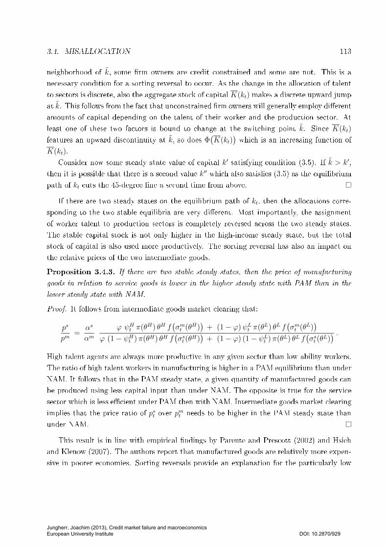
3.4. MISALLOCATION 113
neighborhood of k, some rm owners are credit constrained and some are not. This is a
necessary condition for a sorting reversal to occur. As the change in the allocation of talent
to sectors is discrete, also the aggregate stock of capital K(kt) makes a discrete upward jump
at k. This follows from the fact that unconstrained rm owners will generally employ dierent
amounts of capital depending on the talent of their worker and the production sector. At
least one of these two factors is bound to change at the switching point k. Since K(kt)
features an upward discontinuity at k, so does Φ(K(kt)
)which is an increasing function of
K(kt).
Consider now some steady state value of capital k′ satisfying condition (3.5). If k > k′,
then it is possible that there is a second value k′′ which also satises (3.5) as the equilibrium
path of kt cuts the 45-degree line a second time from above.
If there are two steady states on the equilibrium path of kt, then the allocations corre-
sponding to the two stable equilibria are very dierent. Most importantly, the assignment
of worker talent to production sectors is completely reversed across the two steady states.
The stable capital stock is not only higher in the high-income steady state, but the total
stock of capital is also used more productively. The sorting reversal has also an impact on
the relative prices of the two intermediate goods.
Proposition 3.4.3. If there are two stable steady states, then the price of manufacturing
goods in relation to service goods is lower in the higher steady state with PAM than in the
lower steady state with NAM.
Proof. It follows from intermediate goods market clearing that:
ps
pm=
αs
αmϕ ψHt π(θH) θH f
(σmt (θH)
)+ (1− ϕ)ψLt π(θL) θL f
(σmt (θL)
)ϕ (1− ψHt ) π(θH) θH f
(σst (θ
H))
+ (1− ϕ) (1− ψLt ) π(θL) θL f(σst (θ
L)) .
High talent agents are always more productive in any given sector than low ability workers.
The ratio of high talent workers in manufacturing is higher in a PAM equilibrium than under
NAM. It follows that in the PAM steady state, a given quantity of manufactured goods can
be produced using less capital input than under NAM. The opposite is true for the service
sector which is less ecient under PAM then with NAM. Intermediate goods market clearing
implies that the price ratio of pst over pmt needs to be higher in the PAM steady state than
under NAM.
This result is in line with empirical ndings by Parente and Prescott (2002) and Hsieh
and Klenow (2007). The authors report that manufactured goods are relatively more expen-
sive in poorer economies. Sorting reversals provide an explanation for the particularly low
Jungherr, Joachim (2013), Credit market failure and macroeconomics European University Institute
DOI: 10.2870/929
114 CHAPTER 3. PERSISTENT MISALLOCATION
manufacturing productivity in countries with a low capital stock and low aggregate TFP.
Also the rm size distribution of a given country is aected by assignment reversals.
Proposition 3.4.4. If there are two stable steady states, then the average rm size, measured
in the amount of capital employed, is bigger and the distribution of the rm size is more spread
out in the higher steady state with PAM compared to the lower steady state with NAM.
Proof. The fact that the average rm size is higher is a direct consequence of the higher
stock of capital in the higher steady state.
As the output elasticity εf(σt(θ)
)is a strictly increasing function, PAM will arise if and
only if this results in a higher dispersion of the span of control across rms than under NAM.
It follows that the dispersion of the rm size distribution is also higher under PAM than
with NAM.
The result that credit market frictions compress the ecient plant-size distribution is
common to many models (e.g. Hosono and Takizawa, 2012). Hopenhayn (2012) nds that
the rm-size distributions of India and Mexico, as measured by the number of employees,
are compressed with respect to the U.S. once average rm size is controlled for. China, on
the other hand, does not seem to suer from a similar compression. Alfaro, Charlton and
Kanczuk (2009) nd that the average rm size and its variance are negatively correlated with
per-capita income across countries. This result may be driven by an underrepresentation of
small rms in poor countries in their data set.
3.5 Discussion
We propose a new mechanism to show how credit market failure may give rise to a permanent
misallocation of production factors across sectors and permanent dierences in measured
TFP across countries. At this point, the biggest challenge in this literature is the role of self-
nancing in providing an imperfect substitute for functioning capital markets and thereby
mitigating any long-run eects of nancial frictions for factor allocation and TFP.15 We have
derived our theoretical results within a highly stylized OLG framework. The advantages of
this model with respect to analytical tractability go along with limitations in its capability
to fully address the concerns arising from the mentioned self-nancing channel. It is an
important theoretical question whether sorting reversals of the kind described above may
also give rise to a poverty trap in a model populated by long-lived agents.
15See Banerjee and Moll (2010), Buera, Kaboski and Shin (2011), Moll (2012), Buera and Shin (2013),and Midrigan and Xu (2013).
Jungherr, Joachim (2013), Credit market failure and macroeconomics European University Institute
DOI: 10.2870/929
3.5. DISCUSSION 115
To answer this question, we have to study the assignment of human capital to production
sectors allowing for heterogeneous wealth levels across agents. The matching problem be-
tween rms and workers becomes three-dimensional as some rms own more equity capital
than others. Only a quantitative analysis of sorting reversals in an environment of long-lived
agents can clarify if the existence of poverty traps is robust with respect to the self-nancing
channel. Furthermore, this work would also give an idea about the magnitude of TFP losses
generated by this model along the transition path as well as in a stationary equilibrium.
One implication of sorting reversals is that manufacturing goods may be relatively more
expensive in poor countries than in rich economies. Arguably, capital goods consist to a
higher degree of manufactured goods than consumption goods do. In our model, we have
assumed that capital and consumption goods are produced using identical input shares of
the two intermediate goods. This assumption could be modied to test the robustness of
the results derived above. If capital consists primarily of manufactured goods and if the
manufacturing sector is particularly unproductive at initial stages of economic development,
this would also have an impact on the accumulation of capital and the associated growth
path of the model economy.
Poverty traps may exist in the model described above whenever the constant elasticity
of substitution between capital and labor skill is not exactly unity. However, the model
predictions on sector-specic TFP gaps and on the rm-size distribution across countries
depend on the exact value or at least on the sign of this substitution elasticity. Further
empirical evidence is desirable to inform our parameter choice in this question.
Jungherr, Joachim (2013), Credit market failure and macroeconomics European University Institute
DOI: 10.2870/929
116 CHAPTER 3. PERSISTENT MISALLOCATION
Bibliography
Alfaro, Laura, Andrew Charlton, and Fabio Kanczuk (2009). `Plant-Size Distribution and Cross-CountryIncome Dierences,' in: NBER International Seminar on Macroeconomics 2008, pp. 243-272, University ofChicago Press, Chicago.
Amaral, Pedro S. and Erwan Quintin (2010). `Limited Enforcement, Financial Intermediation, and Eco-nomic Development: A Quantitative Assessment,' International Economic Review, Vol. 51(3), pp. 785-811.
Banerjee, Abhijit V. and Andrew F. Newman (1993). `Occupational Choice and the Process of Develop-ment,' Journal of Political Economy, Vol. 101(2), pp. 274-298.
Banerjee, Abhijit V. and Esther Duo (2005). `Growth Theory through the Lens of Development Economics,'Handbook of Economic Growth, Vol. 1, pp. 473-552.
Banerjee, Abhijit V. and Benjamin Moll (2010). `Why Does Misallocation Persist?' American Economic
Journal: Macroeconomics, Vol. 2(1), pp. 189-206.
Bartelsman, Eric, John Haltiwanger, and Stefano Scarpetta (2013). `Cross-Country Dierences in Produc-tivity: The Role of Allocation and Selection,' The American Economic Review, Vol. 103(1), pp. 305-334.
Beck, Thorsten, Ross Levine, and Norman Loayza (2000). `Finance and the Sources of Growth,' Journal ofFinancial Economics, Vol. 58(1), pp. 261-300.
Beck, Thorsten, Asli Demirgüç-Kunt, and Vojislav Maksimovic (2005). `Financial and Legal Constraints toGrowth: Does Firm Size Matter?' The Journal of Finance, Vol. 60(1), pp. 137-177.
Becker, Gary S. (1973). `A Theory of Marriage: Part I,' Journal of Political Economy, Vol. 81(4), pp.813-846.
Buera, Francisco J. (2008). `Persistency of Poverty, Financial Frictions, and Entrepreneurship,' mimeo, Jan-uary 2008.
Buera, Francisco J., Joseph P. Kaboski, and Yongseok Shin (2011). `Finance and Development: A Tale ofTwo Sectors,' The American Economic Review, Vol. 101(5), pp. 1964-2002.
Buera, Francisco J. and Yongseok Shin (2013). `Financial Frictions and the Persistence of History: A Quan-titative Exploration,' Journal of Political Economy, Vol. 121(2), pp. 221-272.
Caselli, Francesco and Nicola Gennaioli (2013). `Dynastic Management,' Economic Inquiry, Vol. 51(1), pp.971-996.
Costinot, Arnaud (2009). `An Elementary Theory of Comparative Advantage,' Econometrica, Vol. 77(4),pp. 1165-1192.
Erosa, Andrés and Ana Hidalgo Cabrillana (2008). `On Finance as a Theory of TFP, Cross-Industry Pro-ductivity Dierences, and Economic Rents,' International Economic Review, Vol. 49(2), pp. 437-473.
Galor, Oded and Joseph Zeira (1993). `Income Distribution and Macroeconomics,' Review of Economic
Studies, Vol. 60(1), pp. 35-52.
Ghatak, Maitreesh, Massimo Morelli, and Thomas Sjöström (2001). `Occupational Choice and DynamicIncentives,' Review of Economic Studies, Vol. 68(4), pp. 781-810.
Gilchrist, Simon, Jae W. Sim, and Egon Zakraj²ek (2013). `Misallocation and Financial Market Frictions:Some Direct Evidence from the Dispersion in Borrowing Costs,' Review of Economic Dynamics, Vol. 16, pp.159-176.
Jungherr, Joachim (2013), Credit market failure and macroeconomics European University Institute
DOI: 10.2870/929
BIBLIOGRAPHY 117
Giné, Xavier and Robert M. Townsend (2004). `Evaluation of Financial Liberalization: A General Equilib-rium Model with Constrained Occupation Choice,' Journal of Development Economics, Vol. 74, pp. 269-307.
Greenwood, Jeremy, Juan M. Sanchez, and Cheng Wang (2010). `Financing Development: The Role of In-formation Costs,' The American Economic Review, Vol. 100(4), pp. 1875-1891.
Greenwood, Jeremy, Juan M. Sanchez, and Cheng Wang (2013). `Quantifying the Impact of Financial De-velopment on Economic Development,' Review of Economic Dynamics, Vol. 16, pp. 194-215.
Guner, Nezih, Gustavo Ventura, and Yi Xu (2008). `Macroeconomic Implications of Size-Dependent Poli-cies,' Review of Economic Dynamics, Vol. 11, pp. 721-744.
Hamermesh, Daniel S. (1993). Labor Demand, Princeton University Press, Princeton.
Hopenhayn, Hugo A. and Richard Rogerson (1993). `Job Turnover and Policy Evaluation: A General Equi-librium Analysis,' Journal of Political Economy, Vol. 101(5), pp. 915-938.
Hopenhayn, Hugo A. (2012). `On the Measure of Distortions,' mimeo, May 2012.
Hosono, Kaoru and Miho Takizawa (2012). `Do Financial Frictions Matter as a Source of Misallocation?Evidence from Japan,' mimeo, December 2012.
Hsieh, Chang-Tai and Peter J. Klenow (2007). `Relative Prices and Relative Prosperity,' The American
Economic Review, Vol. 97(3), pp. 562-585.
Hsieh, Chang-Tai and Peter J. Klenow (2009). `Misallocation and Manufacturing TFP in China and India,'The Quarterly Journal of Economics, Vol. 124(4), pp. 1403-1448.
Hsieh, Chang-Tai and Peter J. Klenow (2010). `Development Accounting,' American Economic Journal:
Macroeconomics, Vol. 2(1), pp. 207-223.
Jeong, Hyeok and Robert M. Townsend (2007). `Sources of TFP Growth: Occupational Choice and Finan-cial Deepening,' Economic Theory, Vol. 32(1), pp. 179-221.
King, Robert G. and Ross Levine (1993). `Finance and Growth: Schumpeter Might be Right,' The QuarterlyJournal of Economics, Vol. 108(3), pp. 717-737.
Krusell, Per, Lee E. Ohanian, José-Víctor Ríos-Rull, and Giovanni L. Violante (2000). `Capital-Skill Com-plementarity and Inequality: A Macroeconomic Analysis,' Econometrica, Vol. 68(5), pp. 1029-1053.
La Porta, Rafael, Florencio Lopez-de-Silanes, Andrei Shleifer, and Robert W. Vishny (1998). `Law andFinance,' Journal of Political Economy, Vol. 106(6), pp. 1113-1155.
Legros, Patrick and Andrew F. Newman (2002). `Monotone Matching in Perfect and Imperfect Worlds,'Review of Economic Studies, Vol. 69(4), pp. 925-942.
Levine, Ross and Sara Zervos (1998). `Stock Markets, Banks, and Economic Growth,' The American Eco-
nomic Review, Vol. 88(3), pp. 537-558.
Lucas, Robert E. (1978). `On the Size Distribution of Business Firms,' The Bell Journal of Economics, Vol.9(2), pp. 508-523.
Midrigan, Virgiliu and Daniel Yi Xu (2013). `Finance and Misallocation: Evidence from Plant-Level Data,'The American Economic Review, forthcoming.
Moll, Benjamin (2012). `Productivity Losses from Financial Frictions: Can Self-Financing Undo CapitalMisallocation?' mimeo, August 2012.
Jungherr, Joachim (2013), Credit market failure and macroeconomics European University Institute
DOI: 10.2870/929

118 CHAPTER 3. PERSISTENT MISALLOCATION
Mookherjee, Dilip and Debraj Ray (2002). `Contractual Structure and Wealth Accumulation,' The AmericanEconomic Review, Vol. 92(4), pp. 818-849.
Parente, Stephen L. and Edward C. Prescott (2002). Barriers to Riches, MIT Press, Cambridge.
Piketty, Thomas (1997). `The Dynamics of the Wealth Distribution and the Interest Rate with Credit Ra-tioning,' Review of Economic Studies, Vol. 64(2), pp. 173-189.
Rajan, Raghuram G. and Luigi Zingales (1998). `Financial Dependence and Growth,' The American Eco-
nomic Review, Vol. 88(3), pp. 559-586.
Restuccia, Diego and Richard Rogerson (2008). `Policy Distortions and Aggregate Productivity with Het-erogeneous Establishments,' Review of Economic Dynamics, Vol. 11, pp. 707-720.
Rosen, Sherwin (1982). `Authority, Control, and the Distribution of Earnings,' The Bell Journal of Eco-
nomics, Vol. 13(2), pp. 311-323.
Sampson, Thomas (2011). `Assignment Reversals: Trade, Skill Allocation and Wage Inequality,' mimeo,June 2011.
Jungherr, Joachim (2013), Credit market failure and macroeconomics European University Institute
DOI: 10.2870/929


![Imperfections in Solids [Autosaved]](https://img.pdfslide.us/doc/110x75/56d6bcc11a28ab30168b54f1/imperfections-in-solids-autosaved.jpg)