Embed Size (px)
Citation preview
CREDIT EXPANSION AND NEGLECTED CRASH RISK∗
MATTHEW BARON AND WEI XIONG
By analyzing 20 developed economies over 1920–2012, we find the followingevidence of overoptimism and neglect of crash risk by bank equity investors duringcredit expansions: (i) bank credit expansion predicts increased bank equity crashrisk, but despite the elevated crash risk, also predicts lower mean bank equityreturns in subsequent one to three years; (ii) conditional on bank credit expansionof a country exceeding a 95th percentile threshold, the predicted excess returnfor the bank equity index in subsequent three years is −37.3%; and (iii) bankcredit expansion is distinct from equity market sentiment captured by dividendyield and yet dividend yield and credit expansion interact with each other to makecredit expansion a particularly strong predictor of lower bank equity returns whendividend yield is low. JEL Codes: G01, G02, G15, G21.
I. INTRODUCTION
The recent financial crisis in 2007–2008 has renewedeconomists’ interest in the causes and consequences of credit ex-pansions. There is now substantial evidence showing that creditexpansions can have severe consequences on the real economy asreflected by subsequent banking crises, housing market crashes,and economic recessions, (e.g., Borio and Lowe 2002, Mian andSufi 2009, Schularick and Taylor 2012, and Lopez-Salido, Stein,and Zakrajsek 2016). However, the causes of credit expansionremain elusive. An influential yet controversial view put forthby Minsky (1977) and Kindleberger (1978) emphasizes overopti-mism as an important driver of credit expansion. According to thisview, prolonged periods of economic booms tend to breed optimism,which in turn leads to credit expansions that can eventually desta-bilize the financial system and the economy. The recent literaturehas proposed various mechanisms that can lead to such optimism,
∗We are grateful to Tobias Adrian, Nick Barberis, Michael Brennan,Markus Brunnermeier, Priyank Gandhi, Sam Hanson, Dirk Hackbarth, RaviJagannathan, Jakub Jurek, Arvind Krishnamurthy, Luc Laeven, David Laib-son, Matteo Maggiori, Alan Moreira, Ulrich Mueller, Tyler Muir, ChristopherPalmer, Alexi Savov, Hyun Song Shin, Jeremy Stein, Motohiro Yogo, JialinYu, and participants in numerous seminars and workshops for helpful discus-sion and comments. We also thank Andrei Shleifer and four anonymous refer-ees for their constructive suggestions. Isha Agarwal provided excellent researchassistance.C© The Authors 2017. Published by Oxford University Press, on behalf of Presidentand Fellows of Harvard College. All rights reserved. For Permissions, please email:[email protected] Quarterly Journal of Economics (2017), 713–764. doi:10.1093/qje/qjx004.Advance Access publication on January 28, 2017.
713
714 QUARTERLY JOURNAL OF ECONOMICS
such as neglected tail risk (Gennaioli, Shleifer, and Vishny 2012,2013), extrapolative expectations (Barberis, Shleifer, and Vishny1998), and this-time-is-different thinking (Reinhart and Rogoff2009).
Greenwood and Hanson (2013) provide evidence that duringcredit booms in the United States, the credit quality of corpo-rate debt issuance deteriorates and this deterioration forecastslower corporate bond excess returns. Although these findings areconsistent with debt holders being overly optimistic at the timeof credit booms—especially their finding that a deterioration incredit quality predicts negative returns for high-yield debt—thelow, but on average positive, forecasted returns for the overallbond markets may also reflect elevated risk appetite of debt hold-ers during credit expansions. The severe consequences of creditexpansions on the whole economy also invite another importantquestion: whether agents in the economy (other than debt holders)recognize the financial instability associated with credit expan-sion at the time of an expansion. While overoptimism might havecaused debt holders to neglect credit risk during credit expan-sions, this may not be true of equity holders—and, in particular,bank shareholders, who often suffer large losses during financialcrises and thus should have strong incentives to forecast the pos-sibility of financial crises.1 On the other hand, a long traditionlinks large credit expansions with overoptimism in equity mar-kets (Kindleberger 1978), even though it is challenging to finddefinitive evidence of excessive equity valuations.
In this article, we address these issues by systematically ex-amining the expectations of equity investors, an important class ofparticipants in financial markets. Specifically, we take advantageof a key property of equity prices—they reveal the knowledge andexpectations of investors who trade and hold shares. By examiningbank equity returns predicted by credit expansion, we can inferwhether bank shareholders anticipate the risk that large creditexpansions often lead to financial distress and whether sharehold-ers demand a risk premium as compensation.
Our data set consists of 20 developed economies with datafrom 1920 to 2012. We focus on the bank lending component of
1. In contrast, bank depositors and creditors are often protected by explicitand implicit government guarantees during financial crises. Even in the absenceof deposit insurance, U.S. depositors in the Great Depression lost only 2.7% ofthe average amount of deposits in the banking system for the years 1930–1933,despite the fact that 39% of banks failed (Calomiris 2010).
CREDIT EXPANSION AND CRASH RISK 715
credit expansions and measure bank credit expansion as the pastthree-year change in the bank credit to GDP ratio in each coun-try, where bank credit is the amount of net new lending from thebanking sector to domestic households and nonfinancial corpora-tions in a given country. We use this measure of credit expansion,which excludes debt securities held outside the banking sector, be-cause data on nonbank credit is historically limited, and becauseprevious studies (e.g., Schularick and Taylor 2012) demonstratethat the change in bank credit is a robust predictor of financialcrises. Furthermore, the build-up of credit on bank balance sheets(rather than financed by nonbank intermediaries or bond mar-kets) poses the most direct risk to the banking sector itself. Thuswe analyze whether equity investors price in these risks.
Our analysis focuses on four questions regarding credit ex-pansion from the perspective of bank equity holders. First, doescredit expansion predict an increase in the crash risk of the bankequity index in subsequent one to three years? As equity pricestend to crash in advance of banking crises, the predictability ofcredit expansion for banking crises does not necessarily implypredictability for equity crashes. By estimating a probit panel re-gression as the baseline analysis together with a series of quantileregressions as robustness checks, we find that credit expansionpredicts a significantly higher likelihood of bank equity crashesin subsequent years.
Our second question is whether the increased equity crashrisk is compensated by higher equity returns on average. Notethat the predictability of bank credit expansion for subsequenteconomic recessions, as documented by Schularick and Taylor(2012), does not necessarily imply that shareholders should earnlower average returns. If shareholders anticipate the increasedlikelihood of crash risk at the time of a bank credit expansion,they could demand higher expected returns by immediately low-ering share prices and thus earn higher future average returnsfrom holding bank stocks. This is a key argument we use to deter-mine whether shareholders anticipate the increased equity crashrisk associated with credit expansions.
We find that one to three years after bank credit expan-sions, despite the increased crash risk, the mean excess returnof the bank equity index is significantly lower rather than higher.Specifically, a one standard deviation increase in credit expan-sion predicts an 11.4 percentage point decrease in subsequentthree-year-ahead excess returns. One might argue that the lower
716 QUARTERLY JOURNAL OF ECONOMICS
returns predicted by bank credit expansion may be caused by acorrelation of bank credit expansion with a lower equity premiumdue to other reasons, such as elevated risk appetite. However,even after controlling for a host of variables known to predict theequity premium—including dividend yield, book to market, infla-tion, term spread, and nonresidential investment to capital—bankcredit expansion remains strong in predicting lower mean returnsof the bank equity index.
Our third question asks what the magnitude of average bankequity returns is during periods of large credit expansions and con-tractions. We find that conditional on credit expansions exceedinga 95th percentile threshold, the mean excess return in subsequenttwo and three years is substantially negative at −17.9% (with at-statistic of −2.02) and −37.3% (with a t-statistic of −2.52), re-spectively. Note that for publicly traded banks, there is no commit-ment of shareholders to hold bank equity through both good andbad times and thus earn the unconditional equity premium. Ouranalysis thus implies that bank shareholders choose to hold bankequity during large credit booms even when the predicted excessreturns are sharply negative. This substantially negative equitypremium cannot be explained simply by elevated risk appetiteand instead points to the presence of overoptimism or neglect ofcrash risk by equity holders during credit expansions.
Our final question is how the sentiment associated with bankcredit expansions differs from and interacts with equity marketsentiment captured by dividend yield, which is a robust predic-tor of mean equity returns and is sometimes taken as a measureof equity market sentiment. Interestingly, although both bankcredit expansion and low dividend yield of the bank equity in-dex strongly predict lower bank equity returns, they have only asmall correlation with one another. Furthermore, credit expansionhas strong predictive power for bank equity crash risk, whereasdividend yield has no such predictive power for bank equity crashrisk. Consistent with the theoretical insight of Simsek (2013), thiscontrast indicates two different types of sentiment—credit expan-sions are associated with neglect of tail risk, while low dividendyield is associated with optimism about the overall distribution offuture economic fundamentals. Nevertheless, they are not inde-pendent predictors of bank equity returns. The predictive powerof credit expansion is minimal when dividend yield is high, butparticularly strong when dividend yield is low. This asymmetricpattern indicates that credit expansion and dividend yield amplify
CREDIT EXPANSION AND CRASH RISK 717
each other to give credit expansion even stronger predictability forbank equity returns when equity market sentiment is high.
As our analysis builds on predicting bank equity returns afterextreme values of bank credit expansion, we have paid particularattention to verifying the robustness of our results along a numberof dimensions. First, we have consistently used past informationin constructing and normalizing the predictor variables at eachtime point throughout our predictive regressions to avoid any look-ahead bias. In particular, the negative excess returns conditionalon large credit expansions are forecasted at each point in timeusing only past information. Second, to avoid potential biases incomputing t-statistics, we take extra caution along the followingdimensions: (i) we use only nonoverlapping equity returns (i.e., wedelete intervening observations so that we are effectively estimat-ing returns on annual, biennial, or triennial data for one-, two-,or three-year-ahead returns, respectively); (ii) we dually clusterstandard errors both on country and time as in Thompson (2011),since returns and credit expansion may each be correlated bothacross countries and over time; and (iii) as a further robustnesstest to account for correlations across countries, we collapse alllarge credit expansions into 19 distinct historical episodes (e.g.,the Great Depression, the 1997–1998 East Asian Crisis, the 2007–2008 financial crisis, and many lesser known episodes involvingsometimes one or many countries) and find statistically signifi-cant negative returns by averaging these historical episodes asdistinct, independent observations. Third, we repeat our analysisin subsamples of geographical regions and time periods and findconsistent results across the subsamples; in particular, the resultshold over the subsample 1950–2003, which excludes the Great De-pression and the 2007–2008 financial crisis. Finally, we examinea variety of alternative regression specifications and variable con-structions to avoid potential concerns of specification optimizing.We obtain consistent results even after using these conservativemeasures and robustness checks.
Our analysis thus demonstrates the clear presence of overop-timism by bank shareholders during bank credit expansions.2 Our
2. In this regard, our analysis echoes some earlier studies regarding the be-liefs of financial intermediaries during the housing boom that preceded the re-cent global financial crisis. Foote, Gerardi, and Willen (2012) argue that beforethe crisis, top investment banks were fully aware of the possibility of a housingmarket crash but “irrationally” assigned a small probability to this possibility.Cheng, Raina, and Xiong (2014) provide direct evidence that employees in the
718 QUARTERLY JOURNAL OF ECONOMICS
findings shed light on several important issues. First, in the af-termath of the recent crisis, an influential view argues that creditexpansion may reflect active risk seeking by bankers as a re-sult of their misaligned incentives with their shareholders (e.g.,Allen and Gale 2000 and Bebchuk, Cohen, and Spamann 2010).Our study suggests that as shareholders do not recognize therisk taken by bankers, such risk taking is not against the will ofthe shareholders and may even be encouraged by them, as sug-gested by Stein (1996), Bolton, Scheinkman, and Xiong (2006), andCheng, Hong, and Scheinkman (2013). In this sense, policies thataim to tighten the corporate governance of banks and financialfirms are unlikely to fully prevent future financial crises causedby bank credit expansions.
Second, our results have implications for the design of fi-nancial regulations and other efforts to prevent future financialcrises. For example, there is increasing recognition by policy mak-ers across the world of the importance of developing early warningsystems of future financial crises. While prices of financial securi-ties are often considered as potential indicators, the overvaluationof bank equity and the neglect of crash risk associated with largecredit expansions suggest that market prices are poor predictorsof financial distress. Similarly, Krishnamurthy and Muir (2016)find that credit spreads in the run-up to historical crises are “ab-normally low”; the same may be said about credit-default swapspreads on U.S. banks in 2006 and early 2007. Thus our analy-sis suggests that the use of market prices for predicting futurefinancial crises (or, for example, for implementing countercyclicalcapital buffers) is limited because market prices do not price inthe risk of financial crises until it is too late. Quantity variablessuch as growth of bank credit to GDP may be more promisingindicators.
The article is structured as follows. Section II describes thedata used in our analysis. Section III presents the main resultsusing credit expansion to predict bank equity returns. Section IVprovides a variety of robustness checks. Finally, Section V con-cludes. We also provide an Online Appendix, which contains ad-ditional details related to data construction, analogous results for
securitization finance industry were more aggressive in buying second homes fortheir personal accounts than some control groups during the housing bubble and,as a result, performed worse.
CREDIT EXPANSION AND CRASH RISK 719
nonfinancial equities in place of bank equities, and additional ro-bustness analysis.
II. DATA
We construct a panel data set for 20 developed economies withquarterly observations from 1920 to 2012. Specifically, for a coun-try to be included in our sample, it must currently be classified asan advanced economy by the International Monetary Fund (IMF)and have at least 40 years of data for both credit expansion andbank equity index returns.3 For 12 countries, the data set is mostlycomplete from around 1920 onward, whereas for eight countriesthe data set is mostly complete from around 1950 onward. Thesample length of each variable for each country can be found inOnline Appendix Table I.
II.A. Data Construction
The data set primarily consists of three types of variables:credit expansion, bank equity index returns, and various controlvariables known to predict the equity premium. The constructionof the data is outlined below, and more detail can be found inOnline Appendix Section I.
1. Credit Expansion. The key explanatory variable in ouranalysis is referred to as credit expansion and is defined as theannualized past three-year percentage point change in bank creditto GDP, where bank credit is credit from the banking sector to do-mestic households and nonfinancial corporations. Note that creditexpansion throughout this article refers to bank credit expansionexcept where specifically noted. It is expressed mathematically as
�
(bank credit
GDP
)t=
( bank creditGDP
)t − ( bank credit
GDP
)t−3
3.
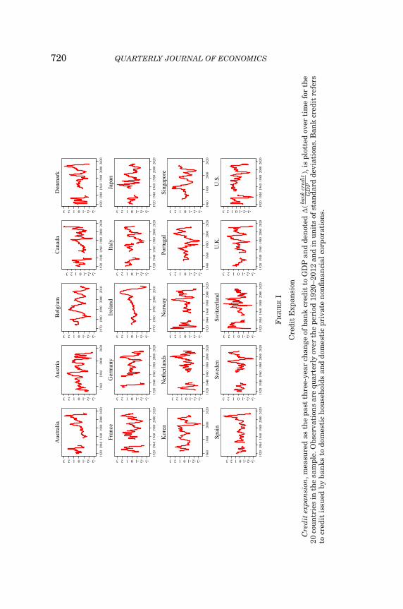
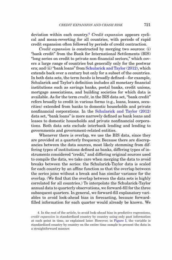
Figure I plots this variable over time for the 20 countriesin the sample, where credit expansion is expressed in standarddeviation units by standardizing it by its mean and standard
3. The latter criterion excludes advanced economies such as Finland, Iceland,and New Zealand, for which there is limited pre-1990s data.
720 QUARTERLY JOURNAL OF ECONOMICS
FIG
UR
EI
Cre
dit
Exp
ansi
on
Cre
dit
expa
nsi
on,m
easu
red
asth
epa
stth
ree-
year
chan
geof
ban
kcr
edit
toG
DP
and
den
oted
�(ba
nkcr
edit
GD
P),
ispl
otte
dov
erti
me
for
the
20co
un
trie
sin
the
sam
ple.
Obs
erva
tion
sar
equ
arte
rly
over
the
peri
od19
20–2
012
and
inu
nit
sof
stan
dard
devi
atio
ns.
Ban
kcr
edit
refe
rsto
cred
itis
sued
byba
nks
todo
mes
tic
hou
seh
olds
and
dom
esti
cpr
ivat
en
onfi
nan
cial
corp
orat
ion
s.
CREDIT EXPANSION AND CRASH RISK 721
deviation within each country.4 Credit expansion appears cycli-cal and mean-reverting for all countries, with periods of rapidcredit expansion often followed by periods of credit contraction.
Credit expansion is constructed by merging two sources: (i)“bank credit” from the Bank for International Settlements (BIS)“long series on credit to private non-financial sectors,” which cov-ers a large range of countries but generally only for the postwarera; and (ii) “bank loans” from Schularick and Taylor (2012), whichextends back over a century but only for a subset of the countries.In both data sets, the term banks is broadly defined—for example,Schularick and Taylor’s definition includes all monetary financialinstitutions such as savings banks, postal banks, credit unions,mortgage associations, and building societies for which data isavailable. As for the term credit, in the BIS data set, “bank credit”refers broadly to credit in various forms (e.g., loans, leases, secu-rities) extended from banks to domestic households and privatenonfinancial corporations. In the Schularick and Taylor (2012)data set, “bank loans” is more narrowly defined as bank loans andleases to domestic households and private nonfinancial corpora-tions. Both data sets exclude interbank lending and lending togovernments and government-related entities.
Whenever there is overlap, we use the BIS data, since theyare provided at a quarterly frequency. Because there are discrep-ancies between the data sources, most likely stemming from dif-fering types of institutions defined as banks, differing types of in-struments considered “credit,” and differing original sources usedto compile the data, we take care when merging the data to avoidbreaks between the series: the Schularick-Taylor data is scaledfor each country by an affine function so that the overlap betweenthe series joins without a break and has similar variance for theoverlap. (We find that the overlap between the data sets is highlycorrelated for all countries.) To interpolate the Schularick-Taylorannual data to quarterly observations, we forward-fill for the threesubsequent quarters. In general, we forward-fill explanatory vari-ables to avoid look-ahead bias in forecasting, because forward-filled information for each quarter would already be known. We
4. In the rest of the article, to avoid look-ahead bias in predictive regressions,credit expansion is standardized country by country using only past informationat each point in time, as explained later. However, in Figure I, the variable isstandardized country by country on the entire time sample to present the data ina straightforward manner.
722 QUARTERLY JOURNAL OF ECONOMICS
do the same for all other predictor variables (e.g., book to market)in cases in which only annual data are given for a variable incertain historical periods.
Our analysis uses the change in bank credit to GDP, ratherthan the level, for the following reasons. The change of credit em-phasizes the cyclicality of credit and represents the amount ofnet new lending to the private sector. When the change in bankcredit is high, the rapid increase in new lending may coincidewith lower lending quality, as shown by Greenwood and Hanson(2013), which may in turn increase subsequent losses in the bank-ing sector and lead to a financial crisis. In contrast to the change,the level of credit exhibits long-term trends presumably relatedto structural and regulatory factors. Differencing bank credit re-moves the secular trend and emphasizes the cyclical movementscorresponding to credit expansions and contractions.5
Because the magnitude of credit expansion varies sub-stantially across countries due to their size and institutionaldifferences, we standardize credit expansion for each countryseparately to make this variable comparable across countries.6
However, to avoid look-ahead bias in the predictability regres-sions, we normalize in such a way that at each time point we useonly past information. That is, for each country and each point intime, we calculate the mean and standard deviation using onlyprior observations in that country and use these values to stan-dardize the given observation.
2. Equity Index Returns. The main dependent variable inour analysis is the future return of the bank equity index for each
5. Why do we choose the past three-year change and not use some otherhorizon? In Online Appendix Table VIII, we provide analysis to show that thegreatest predictive power for subsequent equity returns comes from the secondand third lags in the one-year change in bank credit to GDP, with predictabilitystrongly dropping off at longer lags. It should also be noted that Schularick andTaylor (2012) find similar results for the greatest predictability of future financialcrises with the second and third one-year lags. Thus, we cumulate the three one-year lags to arrive at the past three-year change in bank credit to GDP as themain predictor variable in our analysis.
6. For example, credit expansion in Switzerland has substantially greater vari-ance than in the United States, because Switzerland has a much larger bankingsector relative to GDP. Preliminary tests suggested that it is crucial to standardizeby country: it is the relative size of credit booms relative to the past within a givencountry (perhaps relative to what a country’s institutions are designed to handle)that best predicts returns.
CREDIT EXPANSION AND CRASH RISK 723
country. In Online Appendix Section II, results for the nonfinan-cials equity index are presented, but in all other places we alwaysrefer to the bank equity index for each country. Also, the termreturns always refers to log excess total returns throughout thearticle.7
Our main source for price data for the bank equity index (andfor price and dividend data for the nonfinancials index) is GlobalFinancial Data (GFD). Our main source of bank dividend yielddata is hand-collected data from Moody’s Banking Manuals. Inmany cases, both price and dividend data are supplemented withdata from Compustat, Datastream, and data directly from stockexchange websites and central bank statistics.8 For both banksand nonfinancials, we choose market-capitalization-weighted in-dexes for each country that are as broad as possible within thebanking or nonfinancial sectors (though often, due to limited his-torical data, the nonfinancials index is a broad manufacturing orindustrials index). We compare many historical sources to ensureaccuracy of the historical data. For example, we compare our mainbank price index for each country with several alternative seriesfrom GFD and Datastream, along with an index constructed us-ing hand-collected bank stock prices (annual high and low prices)from Moody’s Manuals; we retain only series that are highly cor-related with other sources (see Online Appendix Table II).
Excess total returns are constructed by taking the quarterlyprice returns, adding in dividend yield, and subtracting the three-month short-term interest rate. For forecasting purposes, we con-struct one-, two-, and three-year-ahead log excess total returns bysumming the consecutive quarterly log returns and applying theappropriate lead operator.
Finally, we also define a crash indicator for one, two, and threeyears ahead for the bank and nonfinancials equity indexes, whichtakes the value of 1 if the log excess total return of the underlyingequity index is less than −30% for any quarter within the one-,two-, or three-year horizon, and 0 otherwise. Analogously, we alsodefine a boom indicator for greater than +30% returns for any
7. We repeat our main results in Online Appendix Table IX with arithmeticequity returns as a robustness check. The results do not meaningfully change.
8. See Online Appendix Section I for additional details on constructing thebank and nonfinancials equity indexes and dividend yield indexes for each coun-try, including links to spreadsheets detailing our source data. Online AppendixSection I also discusses further details regarding the construction of the three-month short-term interest rate, control variables, and other variables.
724 QUARTERLY JOURNAL OF ECONOMICS
quarter within the one-, two-, or three-year horizon. We find thatfor the bank equity index, +30% and −30% quarterly returns hap-pen in roughly 1.1% and 3.2% of quarters, respectively. As thesethreshold values were chosen somewhat arbitrarily, Section IV.Cprovides additional analysis to show that our results on crash riskare robust to using an alternative, quantile-regression approach,which does not rely on the choice of a particular crash definition.9
3. Control Variables. We also employ several financial andmacroeconomic variables, which are known to predict the equitypremium, as controls. The main control variables are dividendyield of the bank equity index,10 book-to-market, inflation, non-residential investment to capital, and term spread. These vari-ables are chosen because the data are available over much of thesample period for the 20 countries and because they have thestrongest predictive power for bank equity index returns in a uni-variate framework.11 Bank dividend yield is trimmed if it exceeds40% annualized (i.e., 10% in a given quarter) to eliminate out-liers. We standardize the control variables across the entire sam-ple pooled across countries and time, which does not introduceforward-looking bias because it is simply a change of units.
4. Other Variables. We also employ various other measuresof aggregate credit of the household, corporate, and financial sec-tors and measures of international credit. Further informationon data sources and variable construction for all variables can befound in the Online Appendix.
II.B. Summary Statistics
Table I presents summary statistics for bank equity index re-turns, nonfinancials equity index returns, credit expansion (i.e.,
9. In unreported results, we verify that our analysis on crash risk is robust tochoosing other thresholds of ±20% or ±25% for booms and crashes.
10. The dividend yield of the entire equity market and smoothed variations ofboth bank and broad market measures are employed in Online Appendix Table VI,which shows that the main results of this article are robust to these alternativemeasures of dividend yield.
11. Online Appendix Table XI analyzes other possible control variables, forwhich there is limited data availability (such as the corporate yield spread andrealized daily volatility) or little predictive power (such as the three-month short-term interest rate [trailing 12-month average], real GDP growth, and sovereigndefault spread) and shows that the addition of these control variables does notmeaningfully change the main results.
CREDIT EXPANSION AND CRASH RISK 725
TA
BL
EI
SU
MM
AR
YS
TA
TIS
TIC
S
Ave
rage
cros
s-co
un
try
NM
ean
Med
ian
Std
.dev
.1%
5%10
%90
%95
%99
%co
rrel
atio
n(w
ith
U.S
.)
Qu
arte
rly
log
retu
rns,
ann
ual
ized
Ban
kin
dex:
exce
ssto
talr
etu
rns
4,15
50.
059
0.04
50.
286
−1.3
76−0
.762
−0.5
070.
597
0.85
71.
803
0.39
4B
ank
inde
x:di
vide
nd
yiel
d4,
155
0.03
70.
036
0.01
90.
000
0.00
80.
014
0.06
00.
067
0.09
30.
305
Non
fin
anci
als
inde
x:ex
cess
tota
lret
urn
s4,
092
0.06
40.
060
0.25
6−1
.266
−0.7
48−0
.518
0.62
70.
856
1.46
10.
411
Mar
ket
inde
x:di
vide
nd
yiel
d4,
092
0.03
60.
033
0.02
00.
008
0.01
30.
016
0.05
90.
068
0.11
70.
606
Cre
dit
topr
ivat
eh
ouse
hol
dsan
dn
onfi
nan
cial
corp
orat
ion
s,pa
stth
ree-
year
ann
ual
ized
perc
enta
ge-p
oin
tch
ange
�(ba
nkcr
edit
GD
P)
4,15
50.
013
0.01
10.
032
−0.0
59−0
.032
−0.0
220.
050
0.06
40.
115
0.22
1
Con
trol
vari
able
s
Infl
atio
n4,
147
0.03
70.
028
0.04
3−0
.076
−0.0
110.
001
0.09
00.
119
0.18
50.
686
Ter
msp
read
4,08
80.
012
0.01
20.
018
−0.0
42−0
.016
−0.0
070.
030
0.03
60.
053
0.18
4B
ook
tom
arke
t2,
437
0.70
70.
621
0.41
60.
265
0.34
10.
377
1.04
21.
333
2.56
40.
543
Inve
stm
ent
toC
apit
al3,
266
0.10
20.
099
0.01
90.
068
0.07
50.
081
0.12
70.
140
0.16
10.
550
Not
es.S
um
mar
yst
atis
tics
are
repo
rted
for
log
tota
lexc
ess
retu
rns
for
both
the
ban
kan
dn
onfi
nan
cial
seq
uit
yin
dexe
s.S
um
mar
yst
atis
tics
are
also
repo
rted
for
the
past
thre
e-ye
arch
ange
inba
nk
cred
itto
GD
Pan
dth
eco
ntr
olva
riab
les.
All
stat
isti
csar
epo
oled
acro
ssco
un
trie
san
dti
me.
Obs
erva
tion
sar
equ
arte
rly
over
the
sam
ple
of20
cou
ntr
ies,
1920
–201
2.
726 QUARTERLY JOURNAL OF ECONOMICS
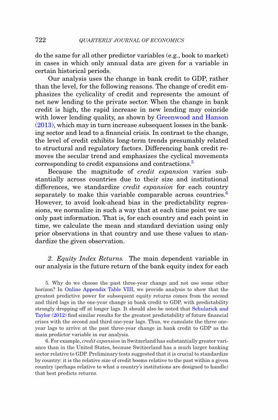
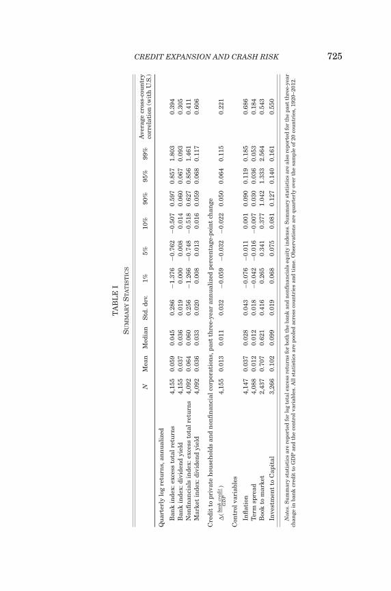
the annualized past three-year change in bank credit to GDP,sometimes denoted mathematically as �( bank credit
GDP )), and controlvariables. Observations are pooled across time and countries.Statistics for returns are all expressed in units of annualized logreturns.
The mean bank and nonfinancials equity index returns are5.9% and 6.4%, respectively, comparable to the historical U.S. eq-uity premium. The standard deviation of bank index returns is28.6%, slightly higher than the standard deviation of 25.6% fornonfinancials. In general, equity returns are moderately corre-lated across countries—bank index returns have an average cor-relation of 0.394 with the United States, and nonfinancials indexreturns have an average correlation of 0.411. Given that this arti-cle studies crash events, it is useful to get a sense of the magnitudeof price drops in various percentiles. The 5th percentile quarterlyreturn, which occurs on average once every five years, is −76.2%(in annualized log terms, thus corresponding to a quarterly dropof −76.2%
4 = 19.1%), and the 1st percentile return is −137.6% (inannualized log terms).
Credit expansion is on average 1.3% a year. In terms of vari-ability, credit expansion grows as rapidly as 6.4 percentage pointsof GDP a year (in the 95th percentile) and contracts as rapidlyas −3.2 percentage points of GDP a year (in the 5th percentile).Table I reports that its time-series correlation with the UnitedStates, averaged across countries, is 0.221. This correlation israther modest, considering that the two most prominent creditexpansions, those leading up to the Great Depression and the2007–2008 financial crisis, were global in nature. In fact, the av-erage correlation of bank credit expansions in 1950–2003 (i.e.,outside of these two episodes) is only 0.109. The relatively id-iosyncratic nature of historical credit expansions, which is alsovisible in Figure I, helps our analysis, as credit expansion’s associ-ations with equity returns and crashes may be attributed largelyto local conditions and not through spillover from crises in othercountries.12
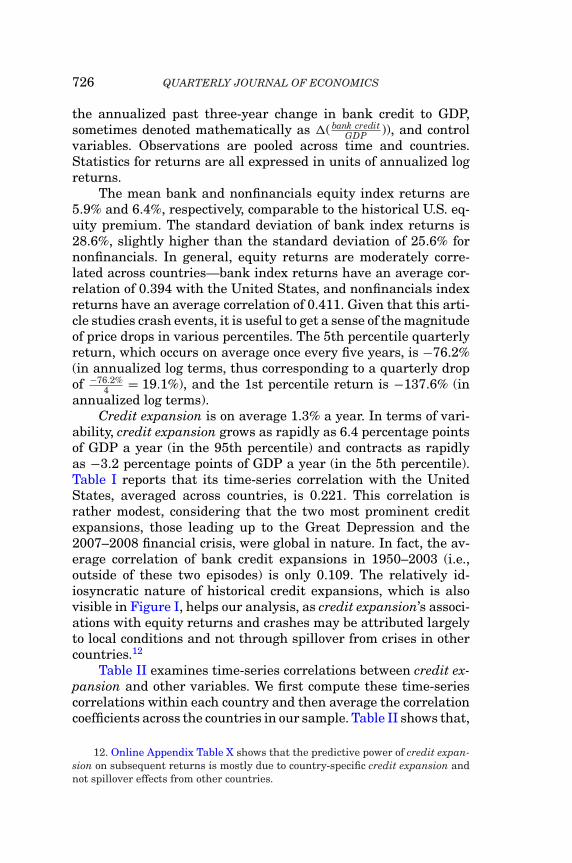
Table II examines time-series correlations between credit ex-pansion and other variables. We first compute these time-seriescorrelations within each country and then average the correlationcoefficients across the countries in our sample. Table II shows that,
12. Online Appendix Table X shows that the predictive power of credit expan-sion on subsequent returns is mostly due to country-specific credit expansion andnot spillover effects from other countries.
CREDIT EXPANSION AND CRASH RISK 727
TABLE IICORRELATIONS
Correlation of �( bank creditGDP ) and: Average correlation Std. err.
�( total creditGDP ) .792∗∗∗ (.048)
�( total credit to HHsGDP ) .636∗∗∗ (.054)
�( total credit to private NFCsGDP ) .608∗∗∗ (.067)
�( bank assetsGDP ) .592∗∗∗ (.056)
Growth of household housing assets .316∗∗∗ (.085)
�( gross external liabilitiesGDP ) .338∗∗∗ (.073)
Current account deficitGDP .172∗∗∗ (.057)
Market dividend yield −.026 (.046)Bank dividend yield .052 (.046)Book to market −.094∗ (.056)Inflation −.103∗∗∗ (.039)Term spread −.136∗∗∗ (.049)Investment to Capital .300∗∗∗ (.070)
Notes. This table reports correlations of the past three-year change in bank credit to GDP with various othermeasures of aggregate credit and with the control variables (market dividend yield, year-over-year inflation,term spread, book to market, and nonresidential investment to capital). Because the measurement of thesevariables may be different from country to country, each correlation is first calculated country by country;then, the correlation coefficient is averaged (and standard errors are calculated) across the 20 countries.∗, ∗∗, and ∗∗∗ denote statistical significance at 10%, 5%, and 1% levels, respectively. Observations are quarterlyover the sample of 20 countries, 1920–2012.
as expected, credit expansion is correlated with changes in otheraggregate credit variables—including total credit (i.e., both bankand nonbank credit), total credit to households, total credit to non-financial corporations, bank assets to GDP, and growth of house-hold housing assets—and with changes in international credit(current account deficits to GDP and changes in gross externalliabilities to GDP), verifying that all these measures of credit gen-erally coincide.13 However, the correlations of credit expansionwith the dividend yield of the bank equity index and with thebroad market index are statistically indistinguishable from zero,which suggests that credit expansion and dividend yield are rela-tively orthogonal variables in predicting future equity returns. Wefurther compare the predictability of bank credit expansion andbank dividend yield in Section III.D and argue that they capturedifferent dimensions of market sentiment.
13. The construction of these variables and their data sources are describedin the Online Appendix.
728 QUARTERLY JOURNAL OF ECONOMICS
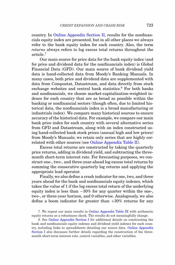
FIGURE II
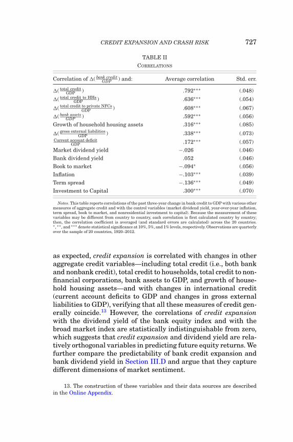
Bank Equity Prices and Bank Credit before and after Large Credit Expansions
The past three-year change in bank credit to GDP (i.e., �( bank creditGDP )) and the
bank total excess log returns index are plotted before and after a large creditexpansion. A large credit expansion is defined as credit expansion exceeding the95th percentile threshold, which is calculated for each country and each point intime using only past information to avoid any future-looking bias. �( bank credit
GDP )and bank total excess log returns are pooled averages across time and countries,conditional on the given number of years before or after the start of a bankingcrisis. The average bank log returns are then cumulated from t = −6 to t = +6,and the level is adjusted to be 0 at t = 0. Observations are over the sample of 20countries, 1920–2012.
II.C. Large Credit Booms and Bank Equity Declines
To understand the timing of credit expansions and bank eq-uity declines, it is useful to plot their dynamics. Figure II depictsthe bank equity index, together with credit expansion, before andafter large credit booms, where a large credit boom is defined asany observation in which credit expansion is above the 95th per-centile relative to past data in that country. We return to thisdefinition in Section III.C.
To produce Figure II, the past three-year change in bankcredit to GDP and bank total excess log returns are averaged,pooled across time and country, conditional on the given num-ber of years before or after a large credit boom (from t = −6 to
CREDIT EXPANSION AND CRASH RISK 729
t = +6). To convert from returns to an index, the average bank logreturns are then cumulated from t = −6 to t = +6, and the levelis adjusted to be 0 at t = 0, the onset of the large credit boom.
The solid curve is the bank equity index (a cumulative logexcess total returns index relative to t = 0, the time of the largecredit boom), and the dashed line is credit expansion (the three-year past change in bank credit to GDP), which reaches a peak ofaround a 7.2 percentage point annualized change in bank creditto GDP at t = 0. In subsequent years after the credit boom, creditexpansion gradually slows down to 0, below its historical trendgrowth rate of 1.3 percentage points; however, when a large creditboom is followed by a banking crisis, as it often is (Borio andLowe 2002; Schularick and Taylor 2012), the decline in creditexpansion is much steeper and turns negative after year two; seeOnline Appendix Figure II for the dynamics of credit expansionand equity prices before and after banking crises.
Figure II previews our main result that credit booms fore-cast large declines in bank equity prices. On average, the equitymarket decline starts around the peak of the credit boom and con-tinues for just over three years. From peak to trough, the averagebank index declines over 30% in log return.14
Figure II also highlights various other aspects of the dynamicsof bank equity prices around large credit booms. For example,Figure II shows how bank equity prices tend to rise considerablyleading up to the peak of the credit boom, with log excess returnsof the bank equity index of 8.5% a year, which is considerablyabove the historical average of 5.9%. Thus, bank equity pricesrise rapidly during the boom years, only to crash on average afterthe peak of the boom.
III. EMPIRICAL RESULTS
Because banks directly suffer from potential defaults of bor-rowers during credit expansions and the risk of a run, bank eq-uity prices should better reflect market expectations of the con-sequences of credit expansions than nonfinancial equity prices.In this section, we report our empirical findings using credit
14. The magnitude of the decline in Figure II is slightly different from theresults in Table V because Table V uses nonoverlapping one-, two-, and three-year-ahead returns for econometric reasons, as explained in Section III. However,the magnitudes are roughly similar.
730 QUARTERLY JOURNAL OF ECONOMICS
expansion to predict both crash risk and mean returns of thebank equity index. We also find similar, albeit less pronounced re-sults from using credit expansion to predict crash risk and equityreturns of nonfinancials; we leave the results for nonfinancials forOnline Appendix Section II.
Our analysis proceeds as follows. We first examine whethercredit expansion predicts an increased equity crash risk in sub-sequent quarters and indeed find supportive evidence. We thenexamine whether credit expansion predicts an increase in meanequity excess returns to compensate investors for the increasedcrash risk and find the opposite result. We examine the magnitudeof the mean equity excess returns and find that conditional on alarge credit expansion, the predicted mean equity excess returnsover subsequent two or three years can be significantly nega-tive. Finally, we compare the sentiment reflected by bank creditexpansion and dividend yield and examine their interaction inpredicting bank equity returns.
Before turning to the regression specifications and estima-tion results, we note two econometric issues, which apply to allthe following analyses. The first is that special care is neededin computing standard errors of these predictive return regres-sions with a financial panel data setting. This is because bothoutcome variables (e.g., K-year-ahead excess returns, K = 1, 2,and 3) and explanatory variables (e.g., credit expansion and con-trols) may be correlated across countries (due to common globalshocks) and over time (due to persistent country-specific shocks).Therefore, we estimate standard errors that are dually clusteredon time and country, following Thompson (2011), to account forboth correlations across countries and over time. For panel linearregression models with fixed effects, that is, equations (2) and (3),we implement dually clustered standard errors by using Whitestandard errors adjusted for clustering on time and country sep-arately, and then combined into a single standard error estimateas explicitly derived in Thompson (2011). For the probit regres-sion, that is, equation (1), and the quantile regressions specifiedin Section IV.C, we estimate dually clustered standard errors byblock bootstrapping, drawing blocks that preserve the correlationstructure both across time and country.
Second, due to well-known econometric issues arising fromusing overlapping returns as the dependent variable (Hodrick1992; Ang and Bekaert 2007), we also take a deliberately con-servative approach by using nonoverlapping returns throughout
CREDIT EXPANSION AND CRASH RISK 731
the analysis. That is, in calculating one-, two-, or three-year-aheadreturns, we drop the intervening observations from our data set,in effect estimating the regressions on annual, biennial, or trien-nial data.15 As a result, we can assume that autocorrelation inthe dependent variables (excess returns) is likely to be minimal.Using nonoverlapping returns thus makes our estimation robustto many potential econometric issues involved in estimating stan-dard errors of overlapping returns.
To carry out the regression analyses, we collect the seriesof credit expansion and bank equity index returns together ina final consolidated data set. Observations are included only ifboth credit expansion and bank equity index returns are nonmiss-ing.16 This gives us a total of 4,155 quarterly observations. Afterdeleting intervening observations to create nonoverlapping one-,two-, or three-year- ahead returns, there are 957, 480, and 316observations for the one-, two-, and three-year-ahead regressions,respectively.
III.A. Predicting Crash Risk
We first estimate probit regressions with an equity crash in-dicator as the dependent variable to examine whether credit ex-pansion predicts increased crash risk. Specifically, we estimatethe following probit model, which predicts future equity crashesusing credit expansion and various controls:
Pr[Yi,t = 1|(predictor variables)i,t]
= �[αiK + βK′(predictor variables)i,t],(1)
where � is the c.d.f. of the standard normal distribution and Y= 1crash is a future crash indicator, which takes on a value of 1
15. Specifically, we look at returns from close December 31, 1919, to closeDecember 31, 1920, and so on, for the one-year-ahead returns; from close December31, 1919, to close December 31, 1921, and so on, for the two-year-ahead returns;and from close December 31, 1919, to close December 31, 1922, and so on, for thethree-year-ahead returns.
16. Given that the control variables are sometimes missing for certain coun-tries and time periods due to historical limitations, missing values for controlvariables are imputed using each country’s mean, where the mean is calculated ateach point in time using only past information, to avoid any look-ahead bias in thepredictive regressions. As shown in Online Appendix Table XI, mean imputationof control variables has little effect on the regression results but is important inpreventing shifts in sample composition when control variables are added.
732 QUARTERLY JOURNAL OF ECONOMICS
if there is an equity crash in the next K years (K = 1, 2, and3) and 0 otherwise.17 As discussed in Section II.A, we define thecrash indicator to take on the value of 1 if the log excess totalreturn of the underlying equity index is less than −30% for anyquarter within the subsequent one-, two-, or three-year horizon,and 0 otherwise. Given that an increased crash probability maybe driven by increased volatility rather than increased crash riskon the downside, we also estimate equation (1) with Y = 1boom,where 1boom is a symmetrically defined positive tail event, and wecompute the difference in the marginal effects between the twoprobit regressions (probability of a crash minus probability of aboom).18
Table III reports the marginal effects corresponding tocrashes in the bank equity index conditional on a one standarddeviation increase in credit expansion. Regressions are estimatedwith and without the control variables. The blocks of columns inTable III correspond to the one-, two-, and three-year-ahead in-creased probability of a crash event. Each regression is estimatedwith various controls: the first block of rows reports marginaleffects conditional on credit expansion with no controls, the sec-ond block of rows reports marginal effects conditional on bankdividend yield with no controls, the third block of rows reportsmarginal effects conditional on both credit expansion and bankdividend yield, and the last block of rows uses credit expansion
17. Another potential way is to use option data to measure tail risk or, moreprecisely, the market perception of tail risk. However, such data are limited torecent years in most countries. Furthermore, as we will see, the market perceptionof tail risk may be different from the objectively measured tail risk.
18. Probit regressions have been widely used to analyze currency crashes, (e.g.,Frankel and Rose 1996, who define a currency crash as a nominal depreciation ofa currency of at least 25% and use a probit regression approach to examine theoccurrence of such currency crashes in a large sample of developing countries.) Thefinance literature tends to use conditional skewness of daily stock returns to exam-ine equity crashes, (e.g., Chen, Hong, and Stein 2001), but this approach would notwork in the present context. As large credit expansions tend to be followed by largeequity price declines over several quarters, as showed by Figure II, such large eq-uity price declines cannot be simply captured by daily stock returns. Furthermore,as the central limit theorem implies that skewness in daily returns is averagedout in quarterly returns, we opt to define equity crashes directly as large declinesin quarterly stock returns, following the literature on currency crashes. One mightbe concerned that the threshold of −30% is arbitrary. We address this concern byusing a quantile regression approach as a robustness check in Section IV.C. Wealso note that similar results (unreported) hold for −20% and −25% thresholds.
CREDIT EXPANSION AND CRASH RISK 733
TA
BL
EII
IC
RE
DIT
EX
PA
NS
ION
PR
ED
ICT
SIN
CR
EA
SE
DC
RA
SH
RIS
KIN
TH
EB
AN
KE
QU
ITY
IND
EX
1ye
arah
ead
2ye
ars
ahea
d3
year
sah
ead
(1)
(2)
(3)
(4)
(5)
(6)
(7)
(8)
(9)
Cra
shB
oom
Dif
fere
nce
Cra
shB
oom
Dif
fere
nce
Cra
shB
oom
Dif
fere
nce
dum
my
dum
my
dum
my
dum
my
dum
my
dum
my
No
con
trol
s�
(bank
cred
itG
DP
)0.
027∗
∗−0
.003
0.03
0∗∗
0.03
3∗∗∗
−0.0
020.
035∗
∗∗0.
054∗
∗∗−0
.012
∗∗∗
0.06
5∗∗∗
[2.4
0][−
0.46
][2
.24]
[3.1
1][−
0.27
][3
.04]
[4.2
7][−
2.91
][5
.20]
N95
795
795
748
048
048
031
631
631
6
No
con
trol
slo
g(ba
nk
div.
yiel
d)−0
.015
0.00
5−0
.020
−0.0
220.
009
−0.0
30−0
.020
0.00
5−0
.024
[−1.
16]
[0.8
6][−
1.28
][−
1.30
][1
.44]
[−1.
37]
[−0.
98]
[0.4
6][−
0.87
]N
957
957
957
480
480
480
316
316
316
Wit
hba
nk
div.
yiel
das
con
trol
�(ba
nkcr
edit
GD
P)
0.02
9∗∗
−0.0
030.
032∗
∗0.
034∗
∗∗−0
.002
0.03
6∗∗∗
0.05
4∗∗∗
−0.0
12∗∗
∗0.
066∗
∗∗
[2.5
4][−
0.59
][2
.49]
[3.0
4][−
0.30
][2
.95]
[4.1
7][−
3.02
][5
.13]
log(
ban
kdi
v.yi
eld)
−0.0
180.
006
−0.0
23−0
.023
0.00
9−0
.032
−0.0
210.
005
−0.0
26[−
1.33
][1
.01]
[−1.
47]
[−1.
39]
[1.4
8][−
1.46
][−
1.09
][0
.49]
[−0.
96]
N95
795
795
748
048
048
031
631
631
6
Wit
hal
lfive
con
trol
s�
(bank
cred
itG
DP
)0.
026∗
∗∗−0
.003
0.03
0∗∗∗
0.02
7∗∗
−0.0
020.
028∗
0.04
6∗∗∗
−0.0
13∗∗
∗0.
059∗
∗∗
(coe
ff.o
nco
ntr
ols
not
repo
rted
)[3
.03]
[−0.
66]
[2.9
6][2
.21]
[−0.
29]
[1.8
0][3
.11]
[−3.
24]
[3.4
8]N
957
957
957
480
480
480
316
316
316
Not
es.T
his
tabl
ere
port
ses
tim
ates
from
the
prob
itre
gres
sion
mod
elsp
ecifi
edin
equ
atio
n(1
)for
the
ban
keq
uit
yin
dex
insu
bseq
uen
ton
e,tw
o,an
dth
ree
year
s.T
he
mai
nde
pen
den
tva
riab
leis
the
cras
hin
dica
tor
(Y=
1 cra
sh),
wh
ich
take
son
ava
lue
of1
ifth
ere
isa
futu
reeq
uit
ycr
ash
,defi
ned
asa
quar
terl
ydr
opof
−30%
orm
ore,
inth
en
ext
Kye
ars
(K=
1,2,
and
3)an
d0
oth
erw
ise.
Th
ecr
ash
indi
cato
ris
regr
esse
don
�(ba
nkcr
edit
GD
P)a
nd
seve
rals
ubs
ets
ofco
ntr
olva
riab
les
know
nto
pred
ict
the
equ
ity
prem
ium
.Exp
lan
ator
yva
riab
les
are
in
stan
dard
devi
atio
nu
nit
s.A
llre
port
edes
tim
ates
are
mar
gin
alef
fect
s.A
coef
fici
ent
of0.
027,
for
exam
ple,
mea
ns
that
a1
stan
dard
devi
atio
nin
crea
sein
�(ba
nkcr
edit
GD
P)p
redi
cts
a2.
7%in
crea
sein
the
like
lih
ood
ofa
futu
recr
ash
.Th
ista
ble
also
repo
rts
esti
mat
esfr
omeq
uat
ion
(1)w
ith
(Y=
1 boo
m),
asy
mm
etri
call
yde
fin
edri
ght-
tail
even
t,al
ong
wit
hth
edi
ffer
ence
inth
em
argi
nal
effe
cts
betw
een
the
two
prob
itre
gres
sion
s(t
he
prob
abil
ity
ofa
cras
hm
inu
sth
epr
obab
ilit
yof
abo
om).
An
alog
ous
resu
lts
for
the
non
fin
anci
als
equ
ity
inde
xar
ere
port
edin
On
lin
eA
ppen
dix
Tab
leII
I.t-
stat
isti
csin
brac
kets
are
com
pute
dfr
omst
anda
rder
rors
dual
lycl
ust
ered
onco
un
try
and
tim
e.∗ ,
∗∗,a
nd
∗∗∗
den
ote
stat
isti
cal
sign
ifica
nce
at10
%,
5%,a
nd
1%le
vels
,res
pect
ivel
y.O
bser
vati
ons
are
over
the
sam
ple
of20
cou
ntr
ies,
1920
–201
2.
734 QUARTERLY JOURNAL OF ECONOMICS
and all five main control variables (bank dividend yield, book tomarket, term spread, investment to capital, and inflation; coeffi-cients on controls omitted to save space).
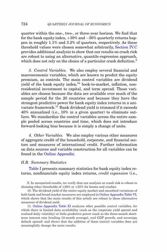
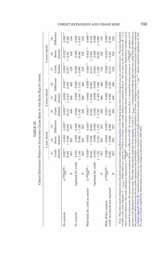
Table III shows that credit expansion predicts an increasedprobability of bank equity crashes. The interpretation of thereported marginal effects is as follows: using the estimates forone-, two-, and three-year-ahead horizons without controls, a onestandard deviation rise in credit expansion is associated withan increase in the probability of a subsequent crash in the bankequity index by 2.7%, 3.3%, and 5.4%, respectively, all statisticallysignificant at the 5% level. (As reference points, the unconditionalprobabilities of a bank equity crash event within the next one,two, and three years are 8.0%, 13.9%, and 19.3%, respectively,so a two standard deviation credit expansion increases theprobability of a crash event by approximately 50%–70%.) Bankdividend yield is not significant in predicting the crash riskof bank equity. More important, the marginal effects of creditexpansion are not affected after adding bank dividend yield andare only slightly reduced, but still significant, after adding all fivecontrols.
To distinguish increased crash risk from the possibility ofincreased return volatility conditional on credit expansion, wesubtract out the marginal effects estimated for a symmetricallydefined positive tail event (i.e., using Y = 1boom as the depen-dent variable). After doing so, the marginal effects stay aboutthe same or actually increase slightly: the probability of a boomconditional on credit expansion tends to decrease, while the prob-ability of a crash increases, suggesting that the probability ofan equity crash subsequent to credit expansion is driven pri-marily by increased negative skewness rather than increasedvolatility of returns. Also, as a robustness check, we adopt analternative measure of crash risk in Section IV.C using a quan-tile regression-based approach, which studies crash risk withoutrelying on a particular choice of thresholds for crash indicatorvariables.
In summary, we find that bank credit expansion predicts anincrease in the crash risk of the bank equity index in the subse-quent one, two, and three years. This result expands the findingsof Borio and Lowe (2002) and Schularick and Taylor (2012) byshowing that credit expansion predicts not only banking crisesbut also bank equity crashes.
CREDIT EXPANSION AND CRASH RISK 735
III.B. Predicting Mean Equity Returns
Given the increased crash risk subsequent to credit expan-sions, we now turn to examining whether the expected returnsof the bank equity index are also higher to compensate equityholders for the increased risk. If bank shareholders recognize theincreased equity crash risk associated with bank credit expan-sions, we expect them to lower current share prices, which in turnwould lead to higher average returns from holding bank stocksdespite the increased equity crash risk in the lower tail.
To examine whether credit expansion predicts higher or lowermean returns, we use an OLS panel regression with country fixedeffects:
(2) ri,t+K − r fi,t+K = αK
i + βK′(predictor variables)i,t + εi,t,
which predicts the K-year ahead excess returns (K = 1, 2, and 3)of the equity index, conditional on a set of predictor variables in-cluding credit expansion. We test whether the coefficient of creditexpansion is different from 0. By using a fixed effects model, wefocus on the time-series dimension within countries.
From an empirical perspective, it is useful to note that creditexpansion may also be correlated with a time-varying equitypremium caused by forces independent of the financial sector,such as by habit formation of representative investors (Campbelland Cochrane 1999) and time-varying long-run consumption risk(Bansal and Yaron 2004). A host of variables are known to predictthe time variation in the equity premium, such as dividend yield,inflation, book to market, term spread, and investment to capital.See Lettau and Ludvigson (2010) for a review of this literature. Itis thus important in our analysis to control for these variables toisolate effects associated with bank credit expansion.
When estimating regressions with bank equity returns, wedo not control for market returns. Although it is true that mar-ket and bank returns are highly correlated and that bank equitycrashes are typically accompanied by contemporaneous declinesin the broad market index, our research question focuses specifi-cally on bank shareholders: why do bank shareholders hold bankstocks during large credit booms when the predicted returns aresharply negative? To study this question, we choose to directly an-alyze how credit expansion predicts bank equity returns, without
736 QUARTERLY JOURNAL OF ECONOMICS
explicitly differentiating the market component versus the bankidiosyncratic component.19
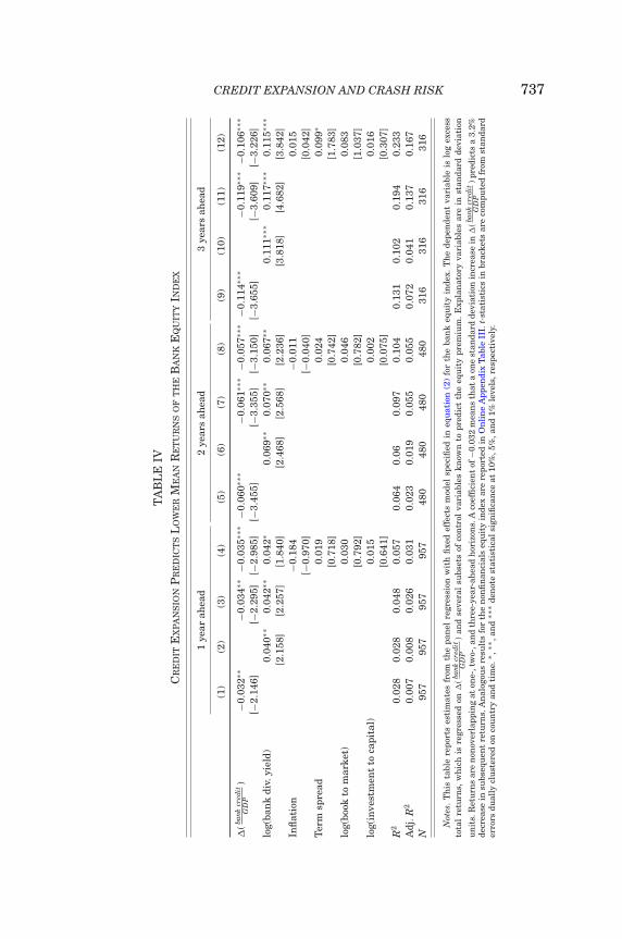
Table IV estimates the panel regression model specified inequation (2). Various columns in Table IV report estimates of re-gressions on credit expansion without controls, with bank dividendyield only, with credit expansion and bank dividend yield together,and with credit expansion and all five main controls (bank divi-dend yield, book to market, term spread, investment to capital,and inflation).
Columns (1)–(4), (5)–(8), and (9)–(12) correspond to resultsassociated with predicting one-, two-, and three-year-ahead ex-cess returns, respectively. Coefficients and t-statistics are re-ported, along with the (within-country) R2 and adjusted R2 forthe mean regressions. A one standard deviation increase in creditexpansion predicts 3.2%, 6.0%, and 11.4% decreases in the subse-quent one-, two-, and three-year-ahead excess returns, respec-tively, all significant at the 5% level. When the controls areincluded, the coefficients are slightly lower but have similar statis-tical significance. In general, coefficients for the mean regressionsare roughly proportional to the number of years, meaning thatthe predictability is persistent and roughly constant per year upto three years.20
Regarding the controls, higher dividend yield, term spread,and book to market are all associated with a higher bank equitypremium (though these coefficients are generally not significantwhen estimated jointly with credit expansion; however, it shouldbe noted that the predictability using these control variables isconsiderably stronger for the nonfinancials equity index than forthe bank equity index, as shown in Online Appendix Table III,which is not surprising). The signs of these coefficients are inline with prior work on equity premium predictability. In partic-ular, bank dividend yield has statistically significant predictivepower for mean excess returns of the bank equity index across all
19. Nevertheless, we verify that the coefficients for the bank equity index arenot higher due to bank stocks having a high market beta. The bank equity indexhas an average market beta of about 1. Also, even after estimating a time-varyingbeta for the bank stock index using daily returns, the idiosyncratic component ofbank returns also exhibits increased crash risk and lower mean returns subse-quent to credit expansion.
20. The coefficients level off after about three years, implying that the pre-dictability is mostly incorporated into returns within three years.
CREDIT EXPANSION AND CRASH RISK 737
TA
BL
EIV
CR
ED
ITE
XP
AN
SIO
NP
RE
DIC
TS
LO
WE
RM
EA
NR
ET
UR
NS
OF
TH
EB
AN
KE
QU
ITY
IND
EX
1ye
arah
ead
2ye
ars
ahea
d3
year
sah
ead
(1)
(2)
(3)
(4)
(5)
(6)
(7)
(8)
(9)
(10)
(11)
(12)
�(ba
nkcr
edit
GD
P)
−0.0
32∗∗
−0.0
34∗∗
−0.0
35∗∗
∗−0
.060
∗∗∗
−0.0
61∗∗
∗−0
.057
∗∗∗
−0.1
14∗∗
∗−0
.119
∗∗∗
−0.1
06∗∗
∗
[−2.
146]
[−2.
295]
[−2.
985]
[−3.
455]
[−3.
355]
[−3.
150]
[−3.
655]
[−3.
609]
[−3.
226]
log(
ban
kdi
v.yi
eld)
0.04
0∗∗
0.04
2∗∗
0.04
2∗0.
069∗
∗0.
070∗
∗0.
067∗
∗0.
111∗
∗∗0.
117∗
∗∗0.
115∗
∗∗
[2.1
58]
[2.2
57]
[1.8
40]
[2.4
68]
[2.5
68]
[2.2
36]
[3.8
18]
[4.6
82]
[3.8
42]
Infl
atio
n−0
.184
−0.0
110.
015
[−0.
970]
[−0.
040]
[0.0
42]
Ter
msp
read
0.01
90.
024
0.09
9∗
[0.7
18]
[0.7
42]
[1.7
83]
log(
book
tom
arke
t)0.
030
0.04
60.
083
[0.7
92]
[0.7
82]
[1.0
37]
log(
inve
stm
ent
toca
pita
l)0.
015
0.00
20.
016
[0.6
41]
[0.0
75]
[0.3
07]
R2
0.02
80.
028
0.04
80.
057
0.06
40.
060.
097
0.10
40.
131
0.10
20.
194
0.23
3A
dj.R
20.
007
0.00
80.
026
0.03
10.
023
0.01
90.
055
0.05
50.
072
0.04
10.
137
0.16
7N
957
957
957
957
480
480
480
480
316
316
316
316
Not
es.
Th
ista
ble
repo
rts
esti
mat
esfr
omth
epa
nel
regr
essi
onw
ith
fixe
def
fect
sm
odel
spec
ified
ineq
uat
ion
(2)
for
the
ban
keq
uit
yin
dex.
Th
ede
pen
den
tva
riab
leis
log
exce
ssto
tal
retu
rns,
wh
ich
isre
gres
sed
on�
(bank
cred
itG
DP
)an
dse
vera
lsu
bset
sof
con
trol
vari
able
skn
own
topr
edic
tth
eeq
uit
ypr
emiu
m.
Exp
lan
ator
yva
riab
les
are
inst
anda
rdde
viat
ion
un
its.
Ret
urn
sar
en
onov
erla
ppin
gat
one-
,tw
o-,a
nd
thre
e-ye
ar-a
hea
dh
oriz
ons.
Aco
effi
cien
tof
−0.0
32m
ean
sth
ata
one
stan
dard
devi
atio
nin
crea
sein
�(ba
nkcr
edit
GD
P)p
redi
cts
a3.
2%de
crea
sein
subs
equ
ent
retu
rns.
An
alog
ous
resu
lts
for
the
non
fin
anci
als
equ
ity
inde
xar
ere
port
edin
On
lin
eA
ppen
dix
Tab
leII
I.t-
stat
isti
csin
brac
kets
are
com
pute
dfr
omst
anda
rder
rors
dual
lycl
ust
ered
onco
un
try
and
tim
e.∗ ,
∗∗,a
nd
∗∗∗
den
ote
stat
isti
cals
ign
ifica
nce
at10
%,5
%,a
nd
1%le
vels
,res
pect
ivel
y.
738 QUARTERLY JOURNAL OF ECONOMICS
horizons and specifications.21 Nevertheless, the coefficient forcredit expansion retains roughly the same magnitude and signifi-cance, despite the controls that are added. Thus, credit expansionadds new predictive power beyond these other variables and is notsimply reflecting another known predictor of the equity premium.
Table IV also reports within-country R2 and adjusted within-country R2 (as both have been reported in the equity premiumpredictability literature). In the univariate framework with justcredit expansion as the predictor, the R2 is 2.8%, 6.4%, and 13.1%for bank returns for one, two, and three years ahead, respectively.Adding the five standard controls increases the R2 to 5.7%, 10.4%,and 23.3% for the same horizons. The relatively modest R2 impliesthat it may be challenging for policy makers to adopt a sharp, real-time policy to avoid the severe consequences of credit expansionand for traders to construct a high Sharpe ratio trading strategybased on credit expansion. Nevertheless, the return predictabilityof credit expansion is strong compared to other predictor variablesexamined in the literature.22
In estimating coefficients for equation (2), we test for thepossible presence of small-sample bias, which may produce biasedestimates of coefficients and standard errors in small samples
21. Note that in Online Appendix Table VI, we use market dividend yield asan alternative control variable. While market dividend yield is perhaps a bettermeasure of the time-varying equity premium in the broad equity market, bankdividend yield performs uniformly better than market dividend yield in predictingboth crash risk and mean excess returns of the bank equity index. Given thatwe are running a horse race between credit expansion and dividend yield, wechoose to use bank dividend yield as the stronger measure to compete againstcredit expansion. Online Appendix Table VI also considers variations on marketdividend yield and bank dividend yield in an effort to “optimize” dividend yield, butnone of these alternatives meaningfully diminish the magnitude and statisticalsignificance of the coefficient on credit expansion.
22. There is a large range of R2 and adjusted R2 values reported in the lit-erature for common predictors of the equity premium in U.S. data. For example,Campbell, Lo, and MacKinlay (1997) report R2 for dividend yield: 0.015, 0.068,0.144 (one, four, eight quarter overlapping horizons, 1927–1994); Lettau and Lud-vigsson (2010) report adjusted R2 for dividend yield: 0.00, 0.01, 0.02, and for cay:0.08, 0.20, 0.28 (one, four, eight quarter overlapping horizons, respectively, 1952–2000); Cochrane (2011) reports R2 for dividend yield: 0.10, for cay and dividendyield together: 0.16, and for investment to capital and dividend yield together: 0.11(for four quarter horizons, 1947–2009); Goyal and Welch (2008) report adjusted R2
of 0.0271, −0.0099, −0.0094, 0.0414, 0.0663, 0.1572 (annual returns, 1927–2005)for dividend yield, inflation, term spread, book to market, investment to capital,and cay, respectively.
CREDIT EXPANSION AND CRASH RISK 739
when a predictor variable is persistent and its innovations arehighly correlated with returns, (e.g., Stambaugh 1999). In OnlineAppendix Section V, we use the methodology of Campbell andYogo (2006) to show that small-sample bias is unlikely to be aconcern for our estimates.
Taken together, the results in Sections III.A and III.B showthat despite the increased crash risk associated with bank creditexpansion, the predicted bank equity excess return is lower ratherthan higher.23 It is important to note that bank credit expansionsare directly observable to the public through central bank statis-tics and banks’ annual reports.24 Thus, it is rather surprisingthat bank shareholders do not demand a higher equity premiumto compensate themselves for the increased crash risk.
III.C. Excess Returns Subsequent to Large Credit Expansionsand Contractions
We further examine the magnitude of predicted bank equityreturns subsequent to “large” credit expansions and contractions.We find that predicted bank equity excess returns subsequentto large credit expansions are significantly negative and large inmagnitude. This analysis helps to isolate the role of overoptimismin driving large credit expansions from that of elevated risk ap-petite, which does not cause the equity premium to go negative.
Specifically, we use a nonparametric model to estimate themagnitude of the predicted equity excess return subsequent to alarge credit expansion:
(3) ri,t+K − r fi,t+K = αK + βK
x · 1{credit expansion>x} + εi,t,
23. Gandhi (2011) also shows that in the U.S. data, aggregate bank creditexpansion negatively predicts the mean return of bank stocks, but he does notexamine the joint presence of increased crash risk subsequent to bank creditexpansions.
24. In all the countries in our sample over the period of 1920–2012, balancesheet information of individual banks was widely available in real time on at leastan annual basis to investors in the form of annual reports (a historical databasecan be found at https://apps.lib.purdue.edu/abldars/); in periodicals such as TheEconomist, Investors Monthly Manual, Bankers Magazine, and so on; and in in-vestor manuals such as the annual Moody’s Banking Manuals (covering banksglobally from 1928 onward) and the International Banking Directory (coveringbanks globally from 1920 onward). In addition to the balance sheets of individualbanks, The Economist and other publications also historically published aggre-gated quarterly or annual statistics of banking sector assets, deposits, loans, andso on.
740 QUARTERLY JOURNAL OF ECONOMICS
where x � 50% is a threshold for credit expansion, ex-pressed in percentiles of credit expansion within a country.We then use the estimates to compute predicted returns:E[ri,t+K − r f
i,t+K | credit expansion > x] = αK + βKx , which we re-
port in Table V. As a benchmark, we often focus on a “large creditexpansion” using the 95th percentile threshold (x = 95%). Toavoid any look-ahead bias, percentile thresholds are calculatedfor each country and each point in time using only past infor-mation. For example, for credit expansion to be above the 95%threshold, credit expansion in that quarter must be greater than95% of all previous observations for that country.
Using this regression model to compute predicted returnsis equivalent to simply computing average excess returns condi-tional on credit expansion exceeding the given percentile thresh-old x.25 The advantage of this formal estimation technique oversimple averaging is that it allows us to compute dually clusteredstandard errors for hypothesis testing, since the error term εi,tis possibly correlated both across time and across countries. Thismodel specification is nonlinear with respect to credit expansionand thus also serves to ensure that our analysis is robust to the lin-ear regression model in equation (2). After estimating this model,we report a t-statistic to test whether the predicted equity pre-mium E[ri,t+K − r f
i,t+K | ·] is significantly different from 0.Furthermore, to examine the predicted equity excess return
subsequent to large credit contractions, we also estimate a sim-ilar model by conditioning on credit contraction, that is, creditexpansion lower than a percentile threshold y � 50%:
(4) ri,t+K − r fi,t+K = αK + βK
y 1{credit expansion<y} + εi,t.
The predicted excess returns conditional on credit expansionexceeding or falling below given percentile thresholds are plot-ted in Figure III and reported in Table V. Specifically, Figure IIIplots the predicted two- and three-year-ahead excess returns con-ditional on credit expansion exceeding various high percentilethresholds varying from the 50th to 98th percentiles and on creditexpansion below various low percentile thresholds from the 2nd
25. Note that equation (3) does not have country fixed effects to avoid look-ahead bias and to be able to compute average returns conditional on a large creditboom. Only without fixed effects is our approach mathematically equivalent tohand-picking all large credit booms and taking a simple average of the subsequentreturns, a fact that can be verified empirically.
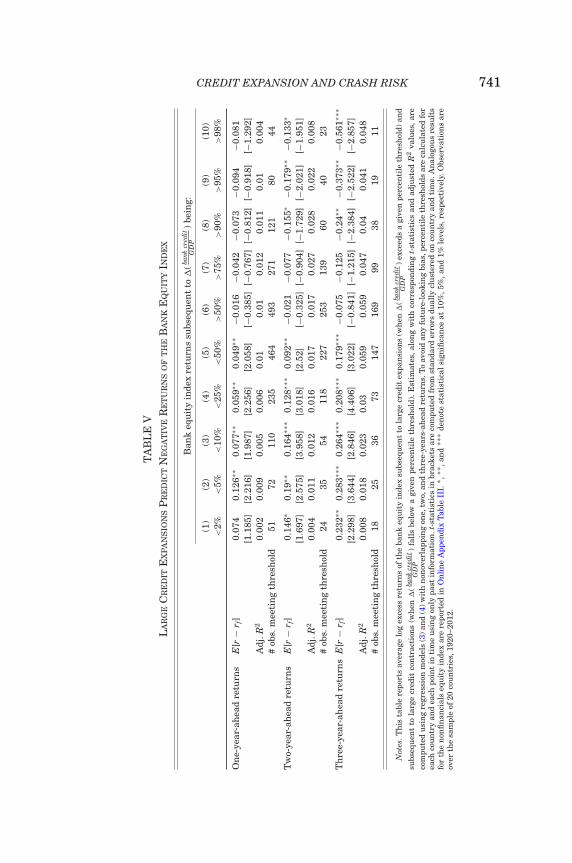
CREDIT EXPANSION AND CRASH RISK 741
TA
BL
EV
LA
RG
EC
RE
DIT
EX
PA
NS
ION
SP
RE
DIC
TN
EG
AT
IVE
RE
TU
RN
SO
FT
HE
BA
NK
EQ
UIT
YIN
DE
X
Ban
keq
uit
yin
dex
retu
rns
subs
equ
ent
to�
(bank
cred
itG
DP
)be
ing:
(1)
(2)
(3)
(4)
(5)
(6)
(7)
(8)
(9)
(10)
<2%
<5%
<10
%<
25%
<50
%>
50%
>75
%>
90%
>95
%>
98%
On
e-ye
ar-a
hea
dre
turn
sE
[r−
r f]
0.07
40.
126∗
∗0.
077∗
∗0.
059∗
∗0.
049∗
∗−0
.016
−0.0
42−0
.073
−0.0
94−0
.081
[1.1
85]
[2.2
16]
[1.9
87]
[2.2
56]
[2.0
58]
[−0.
385]
[−0.
767]
[−0.
812]
[−0.
918]
[−1.
292]
Adj
.R2
0.00
20.
009
0.00
50.
006
0.01
0.01
0.01
20.
011
0.01
0.00
4#
obs.
mee
tin
gth
resh
old
5172
110
235
464
493
271
121
8044
Tw
o-ye
ar-a
hea
dre
turn
sE
[r−
r f]
0.14
6∗0.
19∗∗
0.16
4∗∗∗
0.12
8∗∗∗
0.09
2∗∗
−0.0
21−0
.077
−0.1
55∗
−0.1
79∗∗
−0.1
33∗
[1.6
97]
[2.5
75]
[3.9
58]
[3.0
18]
[2.5
2][−
0.32
5][−
0.90
4][−
1.72
9][−
2.02
1][−
1.95
1]A
dj.R
20.
004
0.01
10.
012
0.01
60.
017
0.01
70.
027
0.02
80.
022
0.00
8#
obs.
mee
tin
gth
resh
old
2435
5411
822
725
313
960
4023
Th
ree-
year
-ah
ead
retu
rns
E[r
−r f
]0.
232∗
∗0.
283∗
∗∗0.
264∗
∗∗0.
208∗
∗∗0.
179∗
∗∗−0
.075
−0.1
25−0
.24∗
∗−0
.373
∗∗−0
.561
∗∗∗
[2.2
98]
[3.6
44]
[2.8
46]
[4.4
06]
[3.0
22]
[−0.
841]
[−1.
215]
[−2.
384]
[−2.
522]
[−2.
857]
Adj
.R2
0.00
80.
018
0.02
30.
030.
059
0.05
90.
047
0.04
0.04
10.
048
#ob
s.m
eeti
ng
thre
shol
d18
2536
7314
716
999
3819
11
Not
es.T
his
tabl
ere
port
sav
erag
elo
gex
cess
retu
rns
ofth
eba
nk
equ
ity
inde
xsu
bseq
uen
tto
larg
ecr
edit
expa
nsi
ons
(wh
en�
(bank
cred
itG
DP
)ex
ceed
sa
give
npe
rcen
tile
thre
shol
d)an
d
subs
equ
ent
tola
rge
cred
itco
ntr
acti
ons
(wh
en�
(bank
cred
itG
DP
)fa
lls
belo
wa
give
npe
rcen
tile
thre
shol
d).
Est
imat
es,
alon
gw
ith
corr
espo
ndi
ng
t-st
atis
tics
and
adju
sted
R2
valu
es,
are
com
pute
du
sin
gre
gres
sion
mod
els
(3)a
nd
(4)w
ith
non
over
lapp
ing
one,
two,
and
thre
e-ye
ars-
ahea
dre
turn
s.T
oav
oid
any
futu
re-l
ooki
ng
bias
,per
cen
tile
thre
shol
dsar
eca
lcu
late
dfo
rea
chco
un
try
and
each
poin
tin
tim
eu
sin
gon
lypa
stin
form
atio
n.t
-sta
tist
ics
inbr
acke
tsar
eco
mpu
ted
from
stan
dard
erro
rsdu
ally
clu
ster
edon
cou
ntr
yan
dti
me.
An
alog
ous
resu
lts
for
the
non
fin
anci
als
equ
ity
inde
xar
ere
port
edin
On
lin
eA
ppen
dix
Tab
leII
I.∗ ,
∗∗,a
nd
∗∗∗
den
ote
stat
isti
cal
sign
ifica
nce
at10
%,5
%,a
nd
1%le
vels
,res
pect
ivel
y.O
bser
vati
ons
are
over
the
sam
ple
of20
cou
ntr
ies,
1920
–201
2.
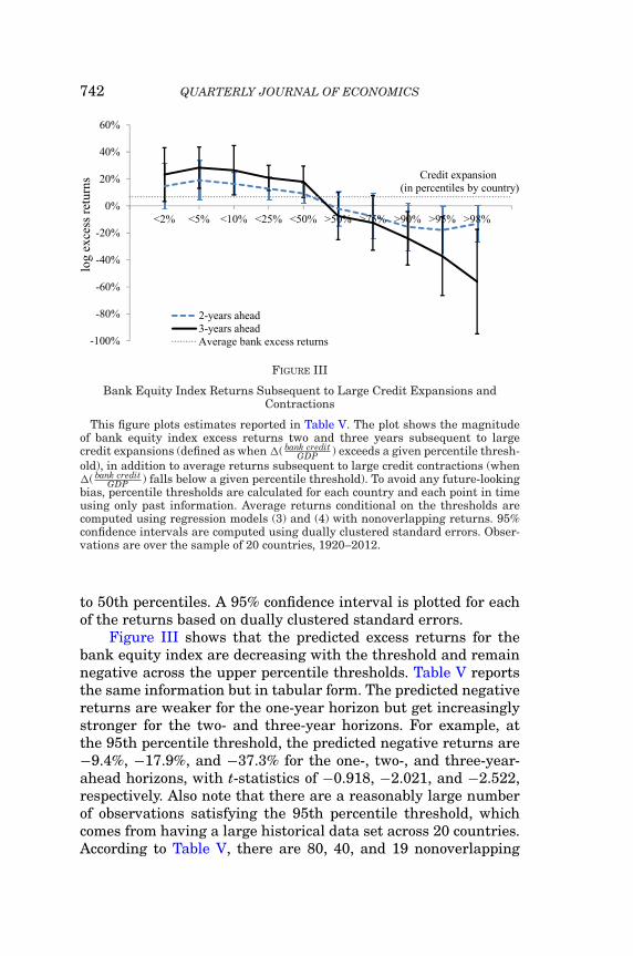
742 QUARTERLY JOURNAL OF ECONOMICS
FIGURE III
Bank Equity Index Returns Subsequent to Large Credit Expansions andContractions
This figure plots estimates reported in Table V. The plot shows the magnitudeof bank equity index excess returns two and three years subsequent to largecredit expansions (defined as when �( bank credit
GDP ) exceeds a given percentile thresh-old), in addition to average returns subsequent to large credit contractions (when�( bank credit
GDP ) falls below a given percentile threshold). To avoid any future-lookingbias, percentile thresholds are calculated for each country and each point in timeusing only past information. Average returns conditional on the thresholds arecomputed using regression models (3) and (4) with nonoverlapping returns. 95%confidence intervals are computed using dually clustered standard errors. Obser-vations are over the sample of 20 countries, 1920–2012.
to 50th percentiles. A 95% confidence interval is plotted for eachof the returns based on dually clustered standard errors.
Figure III shows that the predicted excess returns for thebank equity index are decreasing with the threshold and remainnegative across the upper percentile thresholds. Table V reportsthe same information but in tabular form. The predicted negativereturns are weaker for the one-year horizon but get increasinglystronger for the two- and three-year horizons. For example, atthe 95th percentile threshold, the predicted negative returns are−9.4%, −17.9%, and −37.3% for the one-, two-, and three-year-ahead horizons, with t-statistics of −0.918, −2.021, and −2.522,respectively. Also note that there are a reasonably large numberof observations satisfying the 95th percentile threshold, whichcomes from having a large historical data set across 20 countries.According to Table V, there are 80, 40, and 19 nonoverlapping
CREDIT EXPANSION AND CRASH RISK 743
observations for one-, two-, and three-year-ahead horizons, re-spectively.
Finally, Figure III and Table V also show that subsequent tocredit contractions, the excess returns are positive. When creditcontraction is less than the 5th percentile threshold, the predictedexcess return for the bank equity index in subsequent two andthree years is 19.0% and 28.3%, both significant at the 5% level.26
To sum up, Figure III and Table V document a full picture ofthe time-varying bank equity premium across credit cycles. Theexpected excess return of the bank equity index is substantiallynegative during large bank credit expansions and positive duringlarge contractions.
We provide various robustness checks in Section III to showthat predicted excess returns subsequent to large credit expan-sions are robustly negative: (i) even after grouping concurrentobservations of large credit expansions into distinct episodes andthen averaging across these episodes (addressing the concern thatconcurrent credit expansions in multiple countries during thesame global episode ought to be treated as a single observationrather than separate observations), and (ii) after reanalyzing theresults on various geographical subsets and time subsets (mostimportantly, over the period 1950–2003, showing that the resultsare not simply driven by the Great Depression and the 2007–2008financial crisis).
In the aftermath of the recent financial crisis, a popular viewposits that credit expansion may reflect increased risk appetite offinancial intermediaries due to relaxed value-at-risk constraints(Danielsson, Shin, and Zigrand 2012; Adrian, Moench, and Shin2013). While elevated risk appetite may lead to a reduced equitypremium during periods of credit expansions, it cannot explainthe largely negative bank equity premium reported in Figure IIIand Table V. Instead, this finding suggests the need to incorpo-rate an additional feature that bank shareholders are overly opti-mistic and neglect crash risk during credit expansions. Recently,
26. The large positive returns subsequent to credit contractions may reflectseveral possible mechanisms. First, this pattern is consistent with intermediarycapital losses during credit contraction episodes causing asset market risk premiato rise sharply (e.g., Adrian, Etula, and Muir 2013 and Muir forthcoming). Alter-natively, bank shareholders may systematically underestimate the probability ofa government bailout during the depths of a financial crisis, only to be surprisedlater when a bailout happens.
744 QUARTERLY JOURNAL OF ECONOMICS
Jin (2015) provides a theoretical model to incorporate this impor-tant feature in a dynamic equilibrium model of financial stability.
III.D. Sentiment Reflected by Credit Expansion versus DividendYield
Given the presence of overoptimism during credit expansions,one might naturally wonder how the optimism associated withcredit expansions is related to equity market sentiment. In thissection, we further relate the return predictability of credit expan-sion to that of dividend yield, as the strong predictability of div-idend yield for equity returns is sometimes acknowledged by theliterature as a reflection of equity market sentiment. We are par-ticularly interested in examining whether credit expansion andequity market sentiment may amplify each other in predictingbank equity returns.
We first note that booms in equity and credit markets mightbe driven by different types of sentiment. Credit valuation is par-ticularly sensitive to the belief held by the market about the lowertail risk, while equity valuation is primarily determined by thebelief about the mean or upper end of the distribution of futureeconomic fundamentals. Geanakoplos (2010) develops a tractableframework to analyze credit cycles driven by heterogeneous be-liefs between creditors and borrowers. Simsek (2013) builds onthis framework to show that a credit boom may arise in equilib-rium only when both creditors and borrowers share similar beliefsabout downside states. This credit boom is then able to fuel theoptimism of the borrowers about the overall distribution and leadto an asset market boom.
Simsek’s analysis generates two particularly relevant pointsfor our study. First, a credit boom is mainly determined by thebeliefs of both creditors and borrowers about the lower tail statesand can occur without necessarily being accompanied by an over-all asset market boom. The negligible correlation between creditexpansion and bank dividend yield, as shown by Table II, nicelyconfirms this insight. More important, as shown by Table III,credit expansion has strong predictive power for bank equity crashrisk, while dividend yield has no such predictive power. Further-more, Online Appendix Figure III plots average bank equity indexreturns subsequent to high values of bank dividend yield (whenit exceeds a given percentile threshold) and low values (whenbank dividend yield falls below a given percentile threshold),
CREDIT EXPANSION AND CRASH RISK 745
similar to Figure III but with bank dividend yield rather thancredit expansion. This figure shows that conditional on bank div-idend yield being lower than its 2nd or 5th percentile value, thepredicted returns are somewhat negative in magnitude thoughnot significantly different from zero. These observations aboutthe predictability of bank dividend yield all contrast with creditexpansion, indicating that the sentiment associated with creditexpansions is distinct from equity market sentiment.
Second, when a credit boom occurs together with overopti-mistic beliefs of the borrowers about the upper states of the dis-tribution of future economic fundamentals, the borrowers are ableto use leverage to bid up asset prices or, put differently, the pre-dictability of the credit boom for a negative bank equity premiumis particularly strong. This important insight suggests that creditexpansion may interact with bank dividend yield to provide evenstronger predictive power of the bank equity premium, in partic-ular when bank dividend yield is low (i.e., when there is overopti-mism about the overall distribution). We now examine this insightempirically.
Table VI reports estimation results interacting credit expan-sion with bank dividend yield. Specifically, we estimate the fol-lowing specification:
ri,t+K − r fi,t+K = αK
i + βK1 (credit expansion)i,t
+βK2 (bank dividend yield)i,t
+βK3 (interaction)i,t + εi,t,(5)
where the interaction term is either the standard interactionterm (credit expansion × bank dividend yield) or a nonlinearversion interacting credit expansion with quintile dummies forbank dividend yield. As before, the regression is estimated forone-, two-, and three-year horizons (columns (1)–(3), (4)–(6), and(7)–(9), respectively, in Table VI). Coefficients and t-statistics arereported, along with the within-country R2 and adjusted R2 forthe regressions.
In each group of columns corresponding to one-, two-, andthree-year horizons, the first column reports estimates for justcredit expansion and dividend yield with no interaction term (asin Table IV). The second column adds in the standard interac-tion term (credit expansion × bank dividend yield). Althoughthe estimates are small and not significant at the one- and
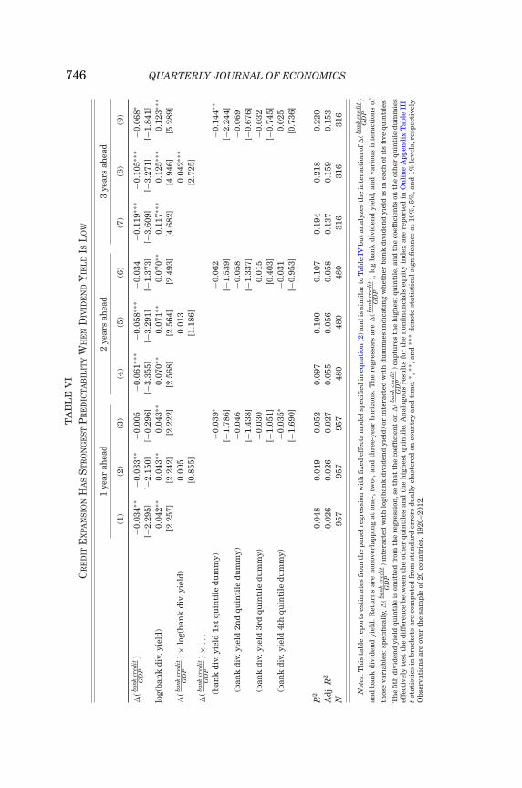
746 QUARTERLY JOURNAL OF ECONOMICST
AB
LE
VI
CR
ED
ITE
XP
AN
SIO
NH
AS
ST
RO
NG
ES
TP
RE
DIC
TA
BIL
ITY
WH
EN
DIV
IDE
ND
YIE
LD
ISL
OW
1ye
arah
ead
2ye
ars
ahea
d3
year
sah
ead
(1)
(2)
(3)
(4)
(5)
(6)
(7)
(8)
(9)
�(ba
nkcr
edit
GD
P)
−0.0
34∗∗
−0.0
33∗∗
−0.0
05−0
.061
∗∗∗
−0.0
58∗∗
∗−0
.034
−0.1
19∗∗
∗−0
.105
∗∗∗
−0.0
68∗
[−2.
295]
[−2.
150]
[−0.
296]
[−3.
355]
[−3.
291]
[−1.
373]
[−3.
609]
[−3.
271]
[−1.
841]
log(
ban
kdi
v.yi
eld)
0.04
2∗∗
0.04
3∗∗
0.04
3∗∗
0.07
0∗∗
0.07
1∗∗
0.07
0∗∗
0.11
7∗∗∗
0.12
5∗∗∗
0.12
3∗∗∗
[2.2
57]
[2.2
42]
[2.2
22]
[2.5
68]
[2.5
64]
[2.4
93]
[4.6
82]
[4.9
46]
[5.2
89]
�(ba
nkcr
edit
GD
P)×
log(
ban
kdi
v.yi
eld)
0.00
50.
013
0.04
2∗∗∗
[0.8
55]
[1.1
86]
[2.7
25]
�(ba
nkcr
edit
GD
P)×
...
(ban
kdi
v.yi
eld
1st
quin
tile
dum
my)
−0.0
39∗
−0.0
62−0
.144
∗∗
[−1.
786]
[−1.
539]
[−2.
244]
(ban
kdi
v.yi
eld
2nd
quin
tile
dum
my)
−0.0
46−0
.058
−0.0
69[−
1.43
8][−
1.33
7][−
0.67
6](b
ank
div.
yiel
d3r
dqu
inti
ledu
mm
y)−0
.030
0.01
5−0
.032
[−1.
051]
[0.4
03]
[−0.
745]
(ban
kdi
v.yi
eld
4th
quin
tile
dum
my)
−0.0
35∗
−0.0
310.
025
[−1.
690]
[−0.
953]
[0.7
36]
R2
0.04
80.
049
0.05
20.
097
0.10
00.
107
0.19
40.
218
0.22
0A
dj.R
20.
026
0.02
60.
027
0.05
50.
056
0.05
80.
137
0.15
90.
153
N95
795
795
748
048
048
031
631
631
6
Not
es.T
his
tabl
ere
port
ses
tim
ates
from
the
pan
elre
gres
sion
wit
hfi
xed
effe
cts
mod
elsp
ecifi
edin
equ
atio
n(2
)an
dis
sim
ilar
toT
able
IVbu
tan
alyz
esth
ein
tera
ctio
nof
�(ba
nkcr
edit
GD
P)
and
ban
kdi
vide
nd
yiel
d.R
etu
rns
are
non
over
lapp
ing
aton
e-,t
wo-
,an
dth
ree-
year
hor
izon
s.T
he
regr
esso
rsar
e�
(bank
cred
itG
DP
),lo
gba
nk
divi
den
dyi
eld,
and
vari
ous
inte
ract
ion
sof
thos
eva
riab
les:
spec
ifica
lly,
�(ba
nkcr
edit
GD
P)
inte
ract
edw
ith
log(
ban
kdi
vide
nd
yiel
d)or
inte
ract
edw
ith
dum
mie
sin
dica
tin
gw
het
her
ban
kdi
vide
nd
yiel
dis
inea
chof
its
five
quin
tile
s.
Th
e5t
hdi
vide
nd
yiel
dqu
inti
leis
omit
ted
from
the
regr
essi
on,s
oth
atth
eco
effi
cien
ton
�(ba
nkcr
edit
GD
P)c
aptu
res
the
hig
hes
tqu
inti
le,a
nd
the
coef
fici
ents
onth
eot
her
quin
tile
dum
mie
sef
fect
ivel
yte
stth
edi
ffer
ence
betw
een
the
oth
erqu
inti
les
and
the
hig
hes
tqu
inti
le.A
nal
ogou
sre
sult
sfo
rth
en
onfi
nan
cial
seq
uit
yin
dex
are
repo
rted
inO
nli
ne
App
endi
xT
able
III.
t-st
atis
tics
inbr
acke
tsar
eco
mpu
ted
from
stan
dard
erro
rsdu
ally
clu
ster
edon
cou
ntr
yan
dti
me.
∗ ,∗∗
,an
d∗∗
∗de
not
est
atis
tica
lsig
nifi
can
ceat
10%
,5%
,an
d1%
leve
ls,r
espe
ctiv
ely.
Obs
erva
tion
sar
eov
erth
esa
mpl
eof
20co
un
trie
s,19
20–2
012.
CREDIT EXPANSION AND CRASH RISK 747
two-year-ahead horizons, the result of 0.042 is sizable and sta-tistically significant at the three-year-ahead horizon. A positivecoefficient is what we expect: a one standard deviation increasein credit expansion combined with a one standard deviation de-crease in dividend yield predicts an interaction effect of lower logexcess returns of 4.2% (that is, beyond what is predicted withcredit expansion and dividend yield individually).
However, the small and insignificant coefficients at the one-and two-year-ahead horizons may be due to the fact that the pre-dictive power of dividend yield is nonlinear and is strongest whendividend yield is very low. We therefore reestimate equation (5) inthe third column with a nonlinear interaction term, interactingcredit expansion with quintile dummies for bank dividend yield.Specifically, we interact credit expansion with the four lowest quin-tile groups, leaving in credit expansion on its own to capture thehighest group. As a result, the coefficients test the interactionsrelative to the omitted group, the highest bank dividend yieldquintile.
In Table VI, the third column shows that in fact the predictivepower of credit expansion is particularly strong when bank divi-dend yield is low, specifically in its lowest quintile: the regressioncoefficient is significantly negative. To interpret the magnitudes,take, for example, the coefficient of −0.039 for the one-year hori-zon. A one standard deviation increase in credit expansion predictsan additional lower mean return of 3.9% when dividend yield is inits lowest quintile relative to its highest quintile (beyond what ispredicted with credit expansion and dividend yield individually).The magnitude is considerably larger, 14.4%, at the three-year-ahead horizon.
Across all the quintiles of bank dividend yield, the coefficientsare statistically significant generally only when bank dividendyield is in the lowest quintile, and its magnitude decreases some-what monotonically across the four dividend yield quintiles. Thissuggests that dividend yield has a nonlinear interaction effectwith credit expansion. When dividend yield is high, the predictivepower of credit expansion is minimal (as shown by the coefficienton the noninteracted credit expansion term, first row). However,when dividend yield is very low (in its lowest quintile), the pre-dictive power of credit expansion is particularly strong.
Overall, we observe that the sentiment associated with creditexpansion is different from equity market sentiment reflected bydividend yield, and yet they interact with each other to give
748 QUARTERLY JOURNAL OF ECONOMICS
credit expansion even stronger predictive power for lower bankequity premium when equity market sentiment is high.
IV. ROBUSTNESS
We present various robustness checks in this section. First,we show that the predicted excess returns subsequent to largecredit expansions remain negative even after robustly accountingfor correlations across time and countries. Second, we show thatthe main results hold on various geographical and time subsets.Finally, we outline a variety of other robustness checks, the resultsof which can be found in the Online Appendix.
IV.A. Clustering Observations by Historical Episodes
Recall Table V, which analyzes equity excess returns subse-quent to large credit expansions and contractions. Approximatelyconcurrent observations of large credit expansions across mul-tiple countries might reflect a single global episode rather thanvarious local events. Accordingly, the episode may have correlatedeffects across countries and over the duration of the episode inways not captured by dually clustered standard errors. Here wedemonstrate that the predicted excess returns subsequent to largecredit expansions are robustly negative, even after grouping obser-vations of large credit expansions into distinct historical episodesand then averaging across these episodes.
Table VII organizes credit expansion observations satisfyingthe 95th percentile threshold into 19 distinct historical episodes.These episodes are widely dispersed throughout the sample pe-riod. Some of them are well known (e.g., the booms preceding theGreat Depression, the Japanese crisis of the 1990s, the Scandi-navian financial crises, the 1997–1998 East Asian crisis, and the2007–2008 global financial crisis), whereas others are less wellknown. Some of these episodes consist of a single country (Japan,1989), and other episodes consist of either a few countries (thelate 1980s booms in Scandinavian countries) or nearly all thecountries in the sample (the 2000s global credit boom). This ro-bustness check first averages large credit expansion observationsacross multiple countries and years that are part of the same his-torical episode, and then considers each of the resulting episodesas a single, independent data point.
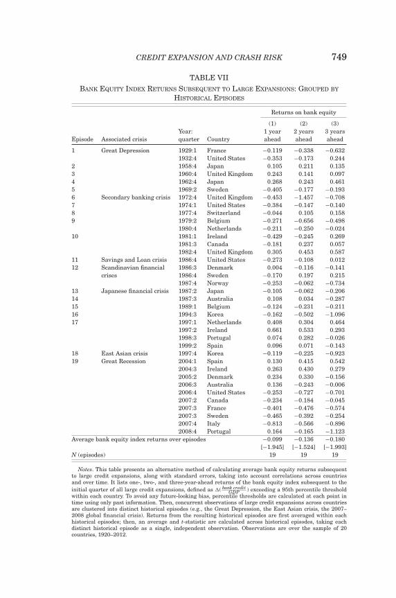
CREDIT EXPANSION AND CRASH RISK 749
TABLE VIIBANK EQUITY INDEX RETURNS SUBSEQUENT TO LARGE EXPANSIONS: GROUPED BY
HISTORICAL EPISODES
Returns on bank equity
(1) (2) (3)Year: 1 year 2 years 3 years
Episode Associated crisis quarter Country ahead ahead ahead
1 Great Depression 1929:1 France −0.119 −0.338 −0.6321932:4 United States −0.353 −0.173 0.244
2 1958:4 Japan 0.105 0.211 0.1353 1960:4 United Kingdom 0.243 0.141 0.0974 1962:4 Japan 0.268 0.243 0.4615 1969:2 Sweden −0.405 −0.177 −0.1936 Secondary banking crisis 1972:4 United Kingdom −0.453 −1.457 −0.7087 1974:1 United States −0.384 −0.147 −0.1408 1977:4 Switzerland −0.044 0.105 0.1589 1979:2 Belgium −0.271 −0.656 −0.498
1980:4 Netherlands −0.211 −0.250 −0.02410 1981:1 Ireland −0.429 −0.245 0.269
1981:3 Canada −0.181 0.237 0.0571982:4 United Kingdom 0.305 0.453 0.587
11 Savings and Loan crisis 1986:4 United States −0.273 −0.108 0.01212 Scandinavian financial 1986:3 Denmark 0.004 −0.116 −0.141
crises 1986:4 Sweden −0.170 0.197 0.2151987:4 Norway −0.253 −0.062 −0.734
13 Japanese financial crisis 1987:2 Japan −0.105 −0.062 −0.20614 1987:3 Australia 0.108 0.034 −0.28715 1989:1 Belgium −0.124 −0.231 −0.21116 1994:3 Korea −0.162 −0.502 −1.09617 1997:1 Netherlands 0.408 0.304 0.464
1997:2 Ireland 0.661 0.533 0.2931998:3 Portugal 0.074 0.282 −0.0261999:2 Spain 0.096 0.071 −0.143
18 East Asian crisis 1997:4 Korea −0.119 −0.225 −0.92319 Great Recession 2004:1 Spain 0.130 0.415 0.542
2004:3 Ireland 0.263 0.430 0.2792005:2 Denmark 0.234 0.330 −0.1562006:3 Australia 0.136 −0.243 −0.0062006:4 United States −0.253 −0.727 −0.7012007:2 Canada −0.234 −0.184 −0.0452007:3 France −0.401 −0.476 −0.5742007:3 Sweden −0.465 −0.392 −0.2542007:4 Italy −0.813 −0.566 −0.8962008:4 Portugal 0.164 −0.165 −1.123
Average bank equity index returns over episodes −0.099 −0.136 −0.180[−1.945] [−1.524] [−1.993]
N (episodes) 19 19 19
Notes. This table presents an alternative method of calculating average bank equity returns subsequentto large credit expansions, along with standard errors, taking into account correlations across countriesand over time. It lists one-, two-, and three-year-ahead returns of the bank equity index subsequent to theinitial quarter of all large credit expansions, defined as �( bank credit
GDP ) exceeding a 95th percentile thresholdwithin each country. To avoid any future-looking bias, percentile thresholds are calculated at each point intime using only past information. Then, concurrent observations of large credit expansions across countriesare clustered into distinct historical episodes (e.g., the Great Depression, the East Asian crisis, the 2007–2008 global financial crisis). Returns from the resulting historical episodes are first averaged within eachhistorical episodes; then, an average and t-statistic are calculated across historical episodes, taking eachdistinct historical episode as a single, independent observation. Observations are over the sample of 20countries, 1920–2012.
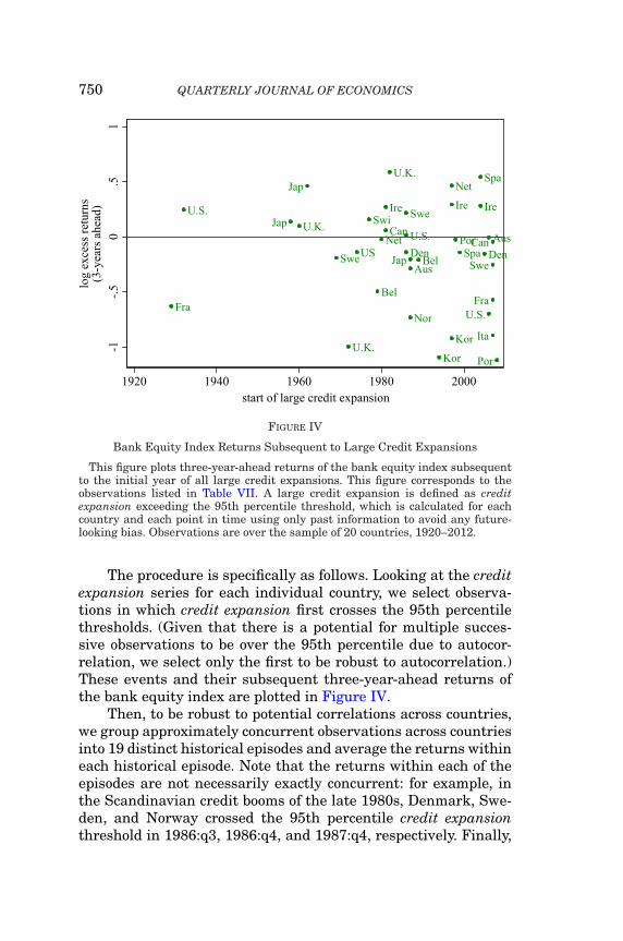
750 QUARTERLY JOURNAL OF ECONOMICS
FIGURE IV
Bank Equity Index Returns Subsequent to Large Credit Expansions
This figure plots three-year-ahead returns of the bank equity index subsequentto the initial year of all large credit expansions. This figure corresponds to theobservations listed in Table VII. A large credit expansion is defined as creditexpansion exceeding the 95th percentile threshold, which is calculated for eachcountry and each point in time using only past information to avoid any future-looking bias. Observations are over the sample of 20 countries, 1920–2012.
The procedure is specifically as follows. Looking at the creditexpansion series for each individual country, we select observa-tions in which credit expansion first crosses the 95th percentilethresholds. (Given that there is a potential for multiple succes-sive observations to be over the 95th percentile due to autocor-relation, we select only the first to be robust to autocorrelation.)These events and their subsequent three-year-ahead returns ofthe bank equity index are plotted in Figure IV.
Then, to be robust to potential correlations across countries,we group approximately concurrent observations across countriesinto 19 distinct historical episodes and average the returns withineach historical episode. Note that the returns within each of theepisodes are not necessarily exactly concurrent: for example, inthe Scandinavian credit booms of the late 1980s, Denmark, Swe-den, and Norway crossed the 95th percentile credit expansionthreshold in 1986:q3, 1986:q4, and 1987:q4, respectively. Finally,
CREDIT EXPANSION AND CRASH RISK 751
the average returns from these episodes are then themselves aver-aged together—taking each such episode as a single, independentobservation—to generate the final average return reported at thebottom of Table VII.
In Table VII and Figure IV, it is important to note that tim-ing the onset of a bank equity crash is difficult, especially whenrestricted to using only past information at each point in time.Therefore, it is to be expected that the timing of events in Ta-ble VII and Figure IV may sometimes look “off.” Observations donot necessarily correspond to the peak of the credit expansion orthe stock market; they are what an observer in real time couldinfer about the credit boom using the 95th percentile rule.27
Even after averaging observations within distinct historicalepisodes and then averaging across these historical episodes, thesubsequent returns are robustly negative. Table VII reports thatthe average excess returns in the one, two, and three years follow-ing the start of historical episodes of large credit expansions are:−9.9%, −13.6%, and −18.0% with t-statistics of −1.945, −1.524,and −1.993, respectively.
IV.B. Robustness in Subsamples
We reestimate the probit (Table III), OLS (Table IV), andnonparametric (Table V) regressions in various geographical andtime subsamples and find that the coefficients have similar mag-nitudes regardless of the subsamples analyzed. The evidencedemonstrates that our results are not driven by any particularsubsets of countries or by specific time periods but hold globallyand, most important, are not simply driven by the Great Depres-sion and the 2007–2008 global financial crisis.
Table VIII, Panels A and B, reports probit marginal effectsand OLS coefficients for credit expansion on future excess returnsof the bank equity index for various subsets of countries and timeperiods. Using a three-year forecasting horizon, the regressionsare analogous to those reported in Tables III and IV. (Resultsalso hold for one- and two-year forecasting horizons.) The sample
27. Many observations in Table VII and Figure IV miss the crash either be-cause the large credit expansion is picked up too early (e.g., Spain 2004) or toolate (e.g., United States 1932). In addition, in the early part of the sample (i.e., thelate 1920s), many credit booms are not picked up at all because there is a limitedhistorical sample on which to calibrate the 95th percentile threshold using onlypast data.
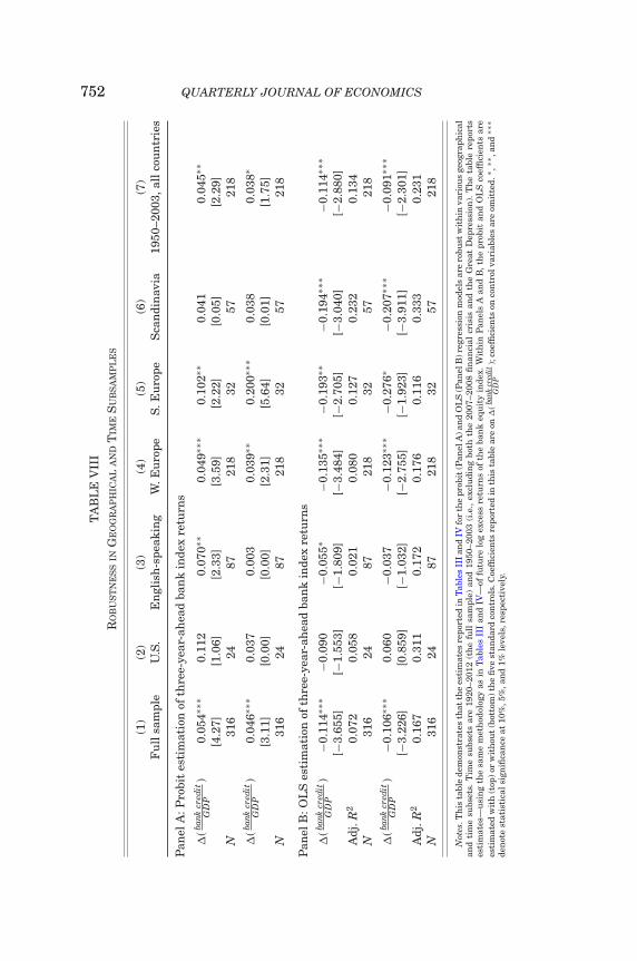
752 QUARTERLY JOURNAL OF ECONOMICST
AB
LE
VII
IR
OB
US
TN
ES
SIN
GE
OG
RA
PH
ICA
LA
ND
TIM
ES
UB
SA
MP
LE
S
(1)
(2)
(3)
(4)
(5)
(6)
(7)
Fu
llsa
mpl
eU
.S.
En
glis
h-s
peak
ing
W.E
uro
peS.
Eu
rope
Sca
ndi
nav
ia19
50–2
003,
allc
oun
trie
s
Pan
elA
:Pro
bit
esti
mat
ion
ofth
ree-
year
-ah
ead
ban
kin
dex
retu
rns
�(ba
nkcr
edit
GD
P)
0.05
4∗∗∗
0.11
20.
070∗
∗0.
049∗
∗∗0.
102∗
∗0.
041
0.04
5∗∗
[4.2
7][1
.06]
[2.3
3][3
.59]
[2.2
2][0
.05]
[2.2
9]N
316
2487
218
3257
218
�(ba
nkcr
edit
GD
P)
0.04
6∗∗∗
0.03
70.
003
0.03
9∗∗
0.20
0∗∗∗
0.03
80.
038∗
[3.1
1][0
.00]
[0.0
0][2
.31]
[5.6
4][0
.01]
[1.7
5]N
316
2487
218
3257
218
Pan
elB
:OL
Ses
tim
atio
nof
thre
e-ye
ar-a
hea
dba
nk
inde
xre
turn
s
�(ba
nkcr
edit
GD
P)
−0.1
14∗∗
∗−0
.090
−0.0
55∗
−0.1
35∗∗
∗−0
.193
∗∗−0
.194
∗∗∗
−0.1
14∗∗
∗[−
3.65
5][−
1.55
3][−
1.80
9][−
3.48
4][−
2.70
5][−
3.04
0][−
2.88
0]A
dj.R
20.
072
0.05
80.
021
0.08
00.
127
0.23
20.
134
N31
624
8721
832
5721
8
�(ba
nkcr
edit
GD
P)
−0.1
06∗∗
∗0.
060
−0.0
37−0
.123
∗∗∗
−0.2
76∗
−0.2
07∗∗
∗−0
.091
∗∗∗
[−3.
226]
[0.8
59]
[−1.
032]
[−2.
755]
[−1.
923]
[−3.
911]
[−2.
301]
Adj
.R2
0.16
70.
311
0.17
20.
176
0.11
60.
333
0.23
1N
316
2487
218
3257
218
Not
es.T
his
tabl
ede
mon
stra
tes
that
the
esti
mat
esre
port
edin
Tab
les
III
and
IVfo
rth
epr
obit
(Pan
elA
)an
dO
LS
(Pan
elB
)reg
ress
ion
mod
els
are
robu
stw
ith
inva
riou
sge
ogra
phic
alan
dti
me
subs
ets.
Tim
esu
bset
sar
e19
20–2
012
(th
efu
llsa
mpl
e)an
d19
50–2
003
(i.e
.,ex
clu
din
gbo
thth
e20
07–2
008
fin
anci
alcr
isis
and
the
Gre
atD
epre
ssio
n).
Th
eta
ble
repo
rts
esti
mat
es—
usi
ng
the
sam
em
eth
odol
ogy
asin
Tab
les
III
and
IV—
offu
ture
log
exce
ssre
turn
sof
the
ban
keq
uit
yin
dex.
Wit
hin
Pan
els
Aan
dB
,th
epr
obit
and
OL
Sco
effi
cien
tsar
ees
tim
ated
wit
h(t
op)o
rw
ith
out
(bot
tom
)th
efi
vest
anda
rdco
ntr
ols.
Coe
ffici
ents
repo
rted
inth
ista
ble
are
on�
(bank
cred
itG
DP
);co
effi
cien
tson
con
trol
vari
able
sar
eom
itte
d.∗ ,
∗∗,a
nd
∗∗∗
den
ote
stat
isti
cals
ign
ifica
nce
at10
%,5
%,a
nd
1%le
vels
,res
pect
ivel
y.
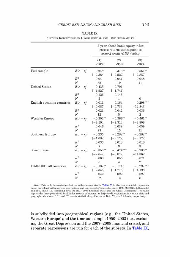
CREDIT EXPANSION AND CRASH RISK 753
TABLE IXFURTHER ROBUSTNESS IN GEOGRAPHICAL AND TIME SUBSAMPLES
3-year-ahead bank equity indexexcess returns subsequent to�(bank credit/GDP) being:
(1) (2) (3)>90% >95% >98%
Full sample E[r − rf] −0.24∗∗ −0.373∗∗ −0.561∗∗[−2.384] [−2.522] [−2.857]
R2 0.04 0.041 0.048N 38 19 11
United States E[r − rf] −0.435 −0.701[−1.527] [−1.741]
R2 0.126 0.146N 2 1 0
English-speaking countries E[r − rf] −0.011 −0.164 −0.298∗∗∗[−0.087] [−0.73] [−12.843]
R2 0.021 0.042 0.036N 12 5 2
Western Europe E[r − rf] −0.302∗∗ −0.369∗∗ −0.561∗∗[−2.194] [−2.314] [−2.808]
R2 0.046 0.038 0.059N 25 15 11
Southern Europe E[r − rf] −0.235 −0.282∗∗ −0.282∗∗[−1.082] [−3.172] [−3.172]
R2 0.033 0.018 0.018N 7 3 3
Scandinavia E[r − rf] −0.353∗∗ −0.474∗∗∗ −0.783∗∗[−2.647] [−5.877] [−14.362]
R2 0.068 0.055 0.071N 8 4 2
1950–2003, all countries E[r − rf] −0.187∗∗ −0.174∗ −0.297∗∗∗[−2.345] [−1.775] [−4.198]
R2 0.042 0.022 0.027N 22 13 8
Notes. This table demonstrates that the estimates reported in Tables V for the nonparametric regressionmodel are robust within various geographical and time subsets. Time subsets are: 1920–2012 (the full sample)and 1950–2003 (i.e., excluding both the 2007–2008 financial crisis and the Great Depression). The tablereports the three-year-ahead bank index returns subsequent to large credit expansions in various time andgeographical subsets. ∗ , ∗∗ , and ∗∗∗ denote statistical significance at 10%, 5%, and 1% levels, respectively.
is subdivided into geographical regions (e.g., the United States,Western Europe) and the time subsample 1950–2003 (i.e., exclud-ing the Great Depression and the 2007–2008 financial crisis), andseparate regressions are run for each of the subsets. In Table IX,
754 QUARTERLY JOURNAL OF ECONOMICS
we reanalyze returns subsequent to large credit expansions (usingthe 95th percentile threshold) for the various subsets.
In Table VIII, we see that the coefficients for the mean andprobit regressions are roughly similar for each of the geographicalsubsets as they are for the full sample of developed countries. TheOLS coefficients are slightly larger for some regions (Southern Eu-rope, Western Europe, Scandinavia) and slightly lower for otherregions (the United States and English-speaking countries). Thestatistical power is reduced for several regions due to the smallersample size of the subsets. The probit coefficients are similar inmagnitude across regions, though with somewhat less statisticalpower, again due to the smaller sample size. In the last column, thecoefficients have almost the same magnitude and statistical sig-nificance over the subperiod 1950–2003, implying that the mainresults are not driven simply by the Great Depression or the 2007–2008 financial crisis.
Table IX shows the average three-year-ahead returns subse-quent to large credit expansions (using the 95th percentile thresh-old) over the various subsets. In general, the coefficients have sim-ilar magnitude regardless of the sample period we use, though thestatistical power is reduced for several subsets due to the oftenmuch smaller sample size. In particular, the results are sharplynegative and statistically significant over the subperiod 1950–2003, again implying that the main results are not driven simplyby the Great Depression or the 2007–2008 financial crisis.
As a related robustness check, Online Appendix Figure IIexamines whether future returns are forecastable at varioustime points historically. This figure presents the coefficient fromthe OLS regressions for three-year-ahead bank index returns(Panel A) and three-year-ahead returns subsequent to large creditexpansions (Panel B) estimated at each point in time t with pastdata up to time t (top plot) and over a rolling past 20-years window(bottom plot). Thus, Online Appendix Figure II can help assesshow these estimates evolved throughout the historical sample andwhat could have been forecastable by investors in real time. SeeOnline Appendix Section IV for further details on methodology.
As one can see in Online Appendix Figure II, the estimateof beta in Panel A is quite stable over the entire sample period,except for a period in the 1950s and early 1960s when the coef-ficient trended upward but subsequently declined. Similarly, theestimate of future three-year-ahead excess returns in Panel B isalso robustly negative, except for a period in the 1950s and early
CREDIT EXPANSION AND CRASH RISK 755
1960s when the past 20-year rolling window saw positive returns.(Perhaps credit booms were not always bad for bank shareholdersin an era of high underlying productivity growth and highly reg-ulated banking.) Thus, Online Appendix Figure II shows that themain results have held since at least the 1980s and, more impor-tant, could have been forecastable at the time by investors duringlarge historical credit expansions.
IV.C. Quantile Regressions as an Alternative Measureof Crash Risk
We use quantile regressions to construct two alternative mea-sures of crash risk subsequent to credit expansion. We use theseapproaches to confirm the results of the probit regression reportedin Table III, that credit expansion predicts increased crash risk ofthe bank equity index. The first approach uses a quantile regres-sion to examine the difference between the predicted mean andmedian (50th quantile) returns—the difference being a measureof crash risk or negative skewness risk—subsequent to credit ex-pansion. The second approach uses quantile regressions to con-struct another measure of negative skewness of future returns,which compares the increase in extreme left-tail events relativeto extreme right-tail events subsequent to credit expansion.
A quantile regression estimates the best linear predictor ofthe qth quantile of future equity excess returns conditional on thepredictor variables:
Quantileq
[ri,t+K − r f
i,t+K | (predictor variables)i,t
](6)
= αKi,q + βK′
q (predictor variables)i,t.
This quantile regression allows one to study how predictor vari-ables forecast the entire shape of the distribution of subsequentexcess returns.
For the first alternative measure of increased crash risk, weanalyze a median regression (50th quantile regression) and com-pare the mean and median excess returns predicted by bank creditexpansions. βmedian estimated from equation (6) measures howmuch bank equity returns decrease “most of the time” during acredit expansion. A negative βmedian indicates that equity excessreturns subsequent to credit expansions are likely to decreaseeven in the absence of the occurrence of crash events. Such a
756 QUARTERLY JOURNAL OF ECONOMICS
negative coefficient reflects gradual correction of equity overvalu-ation induced by shareholders’ overoptimism during credit expan-sions. Thus, the difference between βmean (estimated from equa-tion [2]) and βmedian measures the degree to which crash risk pullsdown the mean returns subsequent to credit expansion.
For the second alternative measure of increased crash risk, weadopt a direct quantile-based approach to study crash risk with-out relying on a particular choice of thresholds for crash indicatorvariables.28 Specifically, we employ jointly estimated quantile re-gressions to compute the following negative skewness statistic toask whether credit expansion predicts increased crash risk:
(7) βnegative skew = (βq=50 − βq=2) − (βq=98 − βq=50),
where βq=x denotes the coefficient estimated for the x quantile.This statistic βnegative skew equals the increased distance from themedian to the lower tail minus the distance to the upper tail,conditional on credit expansion. As with the probit regressions,we do not measure just (βq=50 − βq=2), the distance between themedian and the left tail, because a larger number could sim-ply be indicative of increased conditional variance. Instead, inequation (7), we measure the asymmetry of the return distribu-tion conditional on credit expansion, specifically the increase inthe lower tail minus the increase in the upper tail.29
28. Quantile regression estimates have a slightly different interpretation fromthe probit estimates: the probits analyze the likelihood of tail events, whereasquantile regressions indicate the severity of tail events. It is possible, for example,for the frequency of crash events to stay constant and the severity of such eventsto increase.
29. In the statistics literature, this measure is called the quantile-based mea-sure of skewness. We use the 5th and 95th quantiles to represent tail events,though the results from the quantile regressions are qualitatively similar forvarious other quantiles (for example, 1st/99th or 2nd/98th quantiles) but withslightly less statistical significance. There is a trade-off with statistical power inusing increasingly extreme quantiles, since the number of extreme events getssmaller while the magnitude of the skewness coefficient gets larger. In the caseof testing linear restrictions of coefficients, multiple regressions are estimated si-multaneously to account for correlations in the joint estimates of the coefficients.For example, in testing the null hypothesis H0: βnegative skew = (βq=50 − βq=5)− (βq=95 − βq=50) = 0, standard errors are generated by block bootstrapping si-multaneous estimates of the q = 5, 50, and 95 quantile regressions. Similarly,the difference between the mean and median coefficients, H0: βmean − βmedian =0, is tested by simultaneously bootstrapping mean and median coefficients; theresulting Wald statistic is then used to compute a p-value.
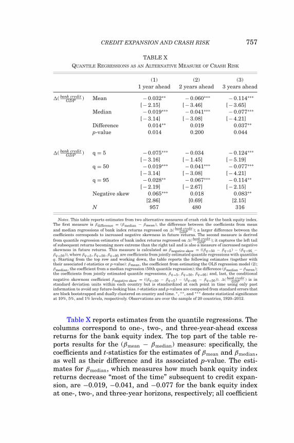
CREDIT EXPANSION AND CRASH RISK 757
TABLE XQUANTILE REGRESSIONS AS AN ALTERNATIVE MEASURE OF CRASH RISK
(1) (2) (3)1 year ahead 2 years ahead 3 years ahead
�( bank creditGDP ) Mean − 0.032∗∗ − 0.060∗∗∗ − 0.114∗∗∗
[ − 2.15] [ − 3.46] [ − 3.65]Median − 0.019∗∗∗ − 0.041∗∗∗ − 0.077∗∗∗
[ − 3.14] [ − 3.08] [ − 4.21]Difference 0.014∗∗ 0.019 0.037∗∗p-value 0.014 0.200 0.044
�( bank creditGDP ) q = 5 − 0.075∗∗∗ − 0.034 − 0.124∗∗∗
[ − 3.16] [ − 1.45] [ − 5.19]q = 50 − 0.019∗∗∗ − 0.041∗∗∗ − 0.077∗∗∗
[ − 3.14] [ − 3.08] [ − 4.21]q = 95 − 0.028∗∗ − 0.067∗∗∗ − 0.114∗∗
[ − 2.19] [ − 2.67] [ − 2.15]Negative skew 0.065∗∗∗ 0.018 0.083∗∗
[2.86] [0.69] [2.15]N 957 480 316
Notes. This table reports estimates from two alternative measures of crash risk for the bank equity index.The first measure is βdifference = (βmedian − βmean), the difference between the coefficients from meanand median regressions of bank index returns regressed on �( bank credit
GDP ); a larger difference between thecoefficients corresponds to increased negative skewness in future returns. The second measure is derivedfrom quantile regression estimates of bank index returns regressed on �( bank credit
GDP ); it captures the left tailof subsequent returns becoming more extreme than the right tail and is also a measure of increased negativeskewness in future returns. This measure is calculated as βnegative skew = ((βq=50 − βq=5) − (βq=95 −βq=50)), where βq=5, βq=50, βq=95 are coefficients from jointly estimated quantile regressions with quantilesq. Starting from the top row and working down, the table reports the following estimates (together withtheir associated t-statistics or p-value): βmean, the coefficient from estimating the OLS regression model (2);βmedian, the coefficient from a median regression (50th quantile regression); the difference (βmedian − βmean);the coefficients from jointly estimated quantile regressions, βq=5, βq=50, βq=95; and, last, the conditionalnegative skewness coefficient βnegative skew = ((βq=50 − βq=5) − (βq=95 − βq=50)). �( bank credit
GDP ) is instandard deviation units within each country but is standardized at each point in time using only pastinformation to avoid any future-looking bias. t-statistics and p-values are computed from standard errors thatare block bootstrapped and dually clustered on country and time. ∗ , ∗∗ , and ∗∗∗ denote statistical significanceat 10%, 5%, and 1% levels, respectively. Observations are over the sample of 20 countries, 1920–2012.
Table X reports estimates from the quantile regressions. Thecolumns correspond to one-, two-, and three-year-ahead excessreturns for the bank equity index. The top part of the table re-ports results for the (βmean − βmedian) measure: specifically, thecoefficients and t-statistics for the estimates of βmean and βmedian,as well as their difference and its associated p-value. The esti-mates for βmedian, which measures how much bank equity indexreturns decrease “most of the time” subsequent to credit expan-sion, are −0.019, −0.041, and −0.077 for the bank equity indexat one-, two-, and three-year horizons, respectively; all coefficient
758 QUARTERLY JOURNAL OF ECONOMICS
estimates are significant at the 1% level. As this decrease in themedian excess return is not related to the occurrence of crashevents, it reflects either the gradual correction of shareholders’overoptimism over time or the elevated risk appetite of share-holders.
(βmean − βmedian) measures how much the mean return isreduced due to the occurrence of tail events in the sample. Ingeneral, the median coefficients are about two-thirds of the levelof corresponding mean coefficients. The remaining third of thedecrease (i.e., βmean − βmedian) reflects the contribution of the oc-currence of crash events in the sample to the change in the meanreturn associated with credit expansion. If shareholders have ra-tional expectations, they would fully anticipate the frequency andseverity of the crash events subsequent to credit expansions andthus demand a higher equity premium ex ante to offset the sub-sequent crashes. To the extent that the median return predictedby credit expansion is lower rather than higher, shareholders donot demand an increased premium to protect them against sub-sequent crash risk.
The bottom part of Table X reports the coefficients andt-statistics for credit expansion from the three quantile re-gressions, βq=5, βq=50, and βq=95, followed by the alternativecrash risk measure—the conditional negative skewness coefficientβnegative skew = (βq=50 − βq=5) − (βq=95 − βq=50)—and its associatedt-statistic. For bank equity index returns, the coefficient for neg-ative skewness, βnegative skew, is estimated to be 0.065, 0.018, and0.083 (the first and third significant at the 5% level) for one-,two-, and three-year horizons, respectively. Overall, the alterna-tive quantile measure of crash risk confirms our earlier findingfrom probit regressions of increased crash risk associated withcredit expansion.
IV.D. Additional Robustness Checks
We perform a variety of other robustness checks in the OnlineAppendix, which we briefly describe below.
1. Test for Possible Small-Sample Bias. Tests of predictabil-ity in equity returns may produce biased estimates of coefficientsand standard errors in small samples when a predictor variable ispersistent and its innovations are highly correlated with returns(e.g., Stambaugh 1999). This small-sample bias could potentially
CREDIT EXPANSION AND CRASH RISK 759
pose a problem for estimating coefficients in our study becausethe main predictor variable, credit expansion, is highly persistenton a quarterly level. In Online Appendix Section V, we test for thepossibility of small-sample bias using the methodology of Camp-bell and Yogo (2006) and find that small-sample bias is not likelyto be a concern for our estimates.
2. “Optimizing” Dividend Yield. Online Appendix Table VIaddresses concerns that perhaps dividend yield does not drive outthe significance of credit expansion because dividend yield is not“optimized” to maximize its predictive power. In Online AppendixTable VI, we therefore consider both market dividend yield andbank dividend yield, with each of those measures also smoothedover the past two, four, or eight quarters. The results with thesealternative dividend yield measures as controls demonstrate thateven “optimizing” dividend yield does not meaningfully dimin-ish the magnitude and statistical significance of the returns pre-dictability of credit expansion.
3. Decomposing the Credit Expansion Measure. Online Ap-pendix Table VII addresses concerns that the predictive powerof �( bank credit
GDP ) might be driven by the denominator (GDP)rather than the numerator (bank credit). However, by breakingdown �( bank credit
GDP ) into �log(bank credit) and �log(GDP) or into�log(real bank credit) and �log(real GDP), Online Appendix Ta-ble VII demonstrates that the predictability in returns is drivenby changes in the numerator (i.e., by �log(bank credit)).
Furthermore, in Online Appendix Table VIII, we motivatethe use of the three-year change in bank credit to GDP by break-ing down this variable into a series of successive one-year changelags. We find that the predictive power of the three-year changein bank credit comes mainly from the second and third one-yearlags: �( bank credit
GDP )t−3,t−2 and �( bank creditGDP )t−2,t−1, dropping off at lags
greater than t – 3. This finding sheds light on the timing of fi-nancial distress, which seems generally to take place at a one- tothree-year horizon subsequent to credit expansion.
4. Robustness in Arithmetic Returns. Online Appendix Ta-ble IX addresses the potential concern that our results mightbe driven by the use of log returns rather than arithmetic re-turns. Although log returns are most appropriate for time-seriesregressions as they reflect compounded returns over time, they
760 QUARTERLY JOURNAL OF ECONOMICS
can accentuate negative skewness. Online Appendix Table IXreplicates the main results of the article but using arithmetic re-turns and shows that the main results (Tables III, IV, V, and VI)are robust to using arithmetic returns as the dependent variable.
5. Global versus Country-Specific Credit Expansions. On-line Appendix Table X addresses concerns that the predictivepower of credit expansion is not due to country-specific credit ex-pansion but from its correlation with a global credit expansion—in other words, that the financial instability comes from spillovereffects from correlated credit expansions in other countries. Al-though this concern would not in any way invalidate this article’sargument that bank shareholders overvalue bank equity and ne-glect tail risk during credit booms, it would suggest that it mightbe more useful to analyze global credit expansion rather thancountry-specific components. Online Appendix Table X shows thatthe predictive power of credit expansion on subsequent returns ismostly due to country-specific effects and not spillover effects fromother countries. To disentangle the effects of local versus globalcredit expansions, we reestimate the regressions in Table IV butcontrol for three additional explanatory variables that measureglobal credit expansion: U.S. credit expansion, U.S. broker-dealerleverage, and the first principal component of credit expansionacross countries, which are all plotted in Online Appendix Table X.U.S. credit expansion has no predictive power for equity returns inother countries, U.S. broker-dealer leverage is a significant pricingfactor for foreign equity returns but does not reduce the predictivepower of local credit expansion, and the first principal componentonly partially reduces the predictive power of local credit expan-sion. We also try various specifications with time fixed effects tocontrol for global average bank returns. As a result, we concludethat the predictive power of credit expansion on subsequent re-turns is in large part due to country-specific credit expansion andnot spillover effects from other countries.
V. CONCLUSION
By analyzing the predictability of bank credit expansion forbank equity index returns in a set of 20 developed economies overthe years 1920–2012, we document empirical evidence support-ing the long-standing view of Minsky (1977) and Kindleberger(1978) regarding overoptimism as an important driver of credit
CREDIT EXPANSION AND CRASH RISK 761
expansion. Specifically, we find that (i) bank credit expansionpredicts increased crash risk in the bank equity index, but de-spite the elevated crash risk, bank credit expansion predicts lowermean bank equity returns in subsequent one to three years; (ii)conditional on bank credit expansion of a country exceeding a95th percentile threshold, the predicted excess return of the bankequity index in subsequent three years is −37.3%, strongly in-dicating the presence of overoptimism and neglect of crash riskat times of rapid credit expansions; (iii) the sentiment associatedwith bank credit expansion is distinct from equity market sen-timent captured by dividend yield, and yet dividend yield andcredit expansion interact with each other to make credit expan-sion a particularly strong predictor of lower bank equity returnswhen dividend yield is low (i.e., when equity market sentiment isstrong).
In the aftermath of the recent financial crisis, an influentialview argues that credit expansion may reflect active risk seekingby bankers as a result of their misaligned incentives with theirshareholders (e.g., Allen and Gale 2000 and Bebchuk, Cohen, andSpamann 2010). Although shareholders may not be able to ef-fectively discipline bankers during periods of rapid bank creditexpansions, they can always vote with their feet and sell theirshares, which would in turn lower equity prices and induce ahigher equity premium to compensate the remaining sharehold-ers for the increased equity risk. In this sense, there does not ap-pear to be an outright tension between shareholders and bankersduring bank credit expansions. Our finding thus implies that bankcredit expansions are not simply caused by bankers acting againstthe will of shareholders. Instead, there is a need to expand thisview by taking into account the presence of overoptimism or ele-vated risk appetite of shareholders.
Our study also has important implications for the pricing oftail risk. Following Rietz (1988) and Barro (2006), a quickly grow-ing body of literature (e.g., Gabaix 2012; Wachter 2013), highlightsrare disasters as a potential resolution of the equity premiumpuzzle. Gandhi and Lustig (2015) argue that greater exposure ofsmall banks to bank-specific tail risk explains the higher equitypremium of small banks. Furthermore, Gandhi (2011) presentsevidence that in the United States, aggregate bank credit expan-sion predicts lower bank returns and argues that this finding isdriven by reduced tail risk during credit expansion. In contrastto this argument, we find increased rather than decreased crash
762 QUARTERLY JOURNAL OF ECONOMICS
risk subsequent to bank credit expansion, which we do by takingadvantage of our large historical data set to forecast rare crashevents. In this regard, our analysis also reinforces the concernexpressed by Chen, Dou, and Kogan (2013) regarding a commonpractice of attributing puzzles in asset prices to “dark matter,”such as tail risk, that is difficult to measure in the data. Our find-ing also suggests that shareholders neglect imminent crash riskduring credit expansions, as pointed out by Gennaioli, Shleifer,and Vishny (2012, 2013). Our analysis does not contradict the im-portance of tail risk in driving the equity premium. Instead, ithighlights that shareholders’ perceived tail risk may or may notbe consistent with realized tail risk, as suggested by Weitzman(2007)—and may even be reversed across credit cycles.
JOHNSON GRADUATE SCHOOL OF MANAGEMENT, CORNELL UNIVERSITY
PRINCETON UNIVERSITY, CHINESE UNIVERSITY OF HONG KONG, SHEN-ZHEN, AND NBER
SUPPLEMENTARY MATERIAL
An Online Appendix for this article can be found at The Quar-terly Journal of Economics online.
REFERENCES
Adrian, Tobias, Erkko Etula, and Tyler Muir, “Financial Intermediaries and theCross-section of Asset Returns,” Journal of Finance, 69 (2013), 2557–2596.
Adrian, Tobias, Emanuel Moench, and Hyun Song Shin, “Leverage Asset Pricing,”Working paper, Princeton University, 2013.
Allen, Franklin, and Douglas Gale, “Bubbles and Crises,” Economic Journal, 110(2000), 236–255.
Ang, Andrew, and Geert Bekaert, “Stock Return Predictability: Is it There?,” Re-view of Financial Studies, 20 (2007), 651–707.
Bansal, Ravi, and Amir Yaron, “Risks for the Long Run: A Potential Resolution ofAsset Pricing Puzzles,” Journal of Finance, 59 (2004), 1481–1509.
Barberis, Nicholas, Andrei Shleifer, and Robert Vishny, “A Model of Investor Sen-timent,” Journal of Financial Economics, 49 (1998), 307–343.
Barro, Robert, “Rare Disasters and Asset Markets in the Twentieth Century,”Quarterly Journal of Economics, 121 (2006), 823–866.
Bebchuk, Lucian, Alma Cohen, and Holger Spamann, “The Wages of Failure: Ex-ecutive Compensation at Bear Stearns and Lehman 2000–2008,” Yale Journalon Regulation, 27 (2010), 257–282.
Bolton, Patrick, Jose Scheinkman, and Wei Xiong, “Executive Compensation andShort-termist Behavior in Speculative Markets,” Review of Economic Studies,73 (2006), 577–610.
Borio, Claudio, and Philip Lowe, “Asset Prices, Financial and Monetary Stability:Exploring the Nexus,” Working paper, Bank for International Settlements,2002.

CREDIT EXPANSION AND CRASH RISK 763
Calomiris, Charles, “The Political Lessons of Depression-Era Banking Reform,”Oxford Review of Economic Policy, 26 (2010), 285–317.
Campbell, John, Andrew Lo, and Craig MacKinlay, The Econometrics of FinancialMarkets (Princeton: Princeton University Press, 1997).
Campbell, John, and John Cochrane, “By Force of Habit: A Consumption-based Ex-planation of Aggregate Stock Market Behavior,” Journal of Political Economy,107 (1999), 205–251.
Campbell, John, and Motohiro Yogo, “Efficient Tests of Stock Return Predictabil-ity,” Journal of Financial Economics, 81 (2006), 27–60.
Chen, Hui, Winston Dou, and Leonid Kogan, “Measuring the ‘Dark Matter’ inAsset Pricing Models,” Working paper, MIT, 2013.
Chen, Joseph, Harrison Hong, and Jeremy C. Stein, “Forecasting Crashes: TradingVolume, Past Returns, and Conditional Skewness in Stock Prices,” Journal ofFinancial Economics, 61 (2001), 345–381.
Cheng, Ing-Haw, Harrison Hong, and Jose Scheinkman, “Yesterday’s Heroes: Com-pensation and Creative Risk-Taking,” Journal of Finance, 70 (2015), 839–879.
Cheng, Ing-Haw, Sahil Raina, and Wei Xiong, “Wall Street and the Housing Bub-ble,” American Economic Review, 104 (2014), 2797–2829.
Cochrane, John, “Presidential address: Discount rates,” Journal of Finance, 66(2011), 1047–1108.
Danielsson, Jon, Hyun Song Shin, and Jean-Pierre Zigrand, “Procyclical Leverageand Endogenous Risk,” Working paper, Princeton University, 2012.
Foote, Christopher, Kristopher Gerardi, and Paul Willen, “Why Did So Many Peo-ple Make So Many Ex-post Bad Decisions? The Causes of the ForeclosureCrisis,” Working paper, Federal Reserve Bank of Boston, 2012.
Frankel, Jeffrey, and Andrew Rose, “Currency Crashes in Emerging Markets: AnEmpirical Treatment,” Journal of international Economics, 41 (1996), 351–366.
Gabaix, Xavier, “Variable Rare Disasters: An Exactly Solved Framework for TenPuzzles in Macro-finance,” Quarterly Journal of Economics, 127 (2012), 645–700.
Gandhi, Priyank, “The Relationship between Credit Growth and the ExpectedReturns of Bank Stocks,” Working paper, UCLA, 2011.
Gandhi, Priyank, and Hanno Lustig, “Size Anomalies in US Bank Stock Returns,”Journal of Finance, 70 (2015), 733–768.
Geanakoplos, John, “The Leverage Cycle,” NBER Macroeconomics Annual 2009,24 (2010), 1–65.
Gennaioli, Nicola, Andrei Shleifer, and Robert Vishny, “Neglected Risks, FinancialInnovation, and Financial Fragility,” Journal of Financial Economics, 104(2012), 452–468.
———, “A Model of Shadow Banking,” Journal of Finance, 68 (2013), 1331–1363.Goyal, Amit, and Ivo Welch, “A Comprehensive Look at the Empirical Performance
of Equity Premium Prediction,” Review of Financial Studies, 21 (2008), 1455–1508.
Greenwood, Robin, and Samuel G. Hanson, “Issuer Quality and Corporate BondReturns,” Review of Financial Studies, 26 (2013), 1483–1525.
Hodrick, Robert, “Dividend Yields and Expected Stock Returns: Alternative Proce-dures for Inference and Measurement,” Review of Financial Studies, 5 (1992),357–386.
Jin, Lawrence, “A Speculative Asset Pricing Model of Financial Instability,” Work-ing paper, Yale University, 2015.
Kindleberger, Charles, Manias, Panics, and Crashes: A History of Financial Crises(New York: Basic Books, 1978).
Krishnamurthy, Arvind, and Tyler Muir, “Credit Spreads and the Severity ofFinancial Crises,” Working paper, Stanford University, 2016.
Lettau, Martin, and Sydney Ludvigson, “Measuring and Modeling Variation inthe Risk-Return Tradeoff,” in Handbook of Financial Econometrics, YacineAit-Sahalia and Lars-Peter Hansen, eds. (Oxford: North-Holland, 2010).
764 QUARTERLY JOURNAL OF ECONOMICS
Lopez-Salido, David, Jeremy Stein, and Egon Zakrajsek, “Credit-Market Senti-ment and the Business Cycle,” NBER Working Paper 21879, 2016.
Mian, Atif, and Amir Sufi, “The Consequences of Mortgage Credit Expansion: Evi-dence from the U.S. Mortgage Default Crisis,” Quarterly Journal of Economics,124 (2009), 1449–1496.
Minsky, Hyman, “The Financial Instability Hypothesis: An Interpretation ofKeynes and an Alternative to ‘Standard’ Theory,” Nebraska Journal of Eco-nomics and Business, 16 (1977), 5–16.
Muir, Tyler, “Financial Crises and Risk Premia,” Quarterly Journal of Economics(forthcoming).
Reinhart, Carmen, and Kenneth Rogoff, This Time Is Different: Eight Centuries ofFinancial Folly (Princeton, NJ: Princeton University Press, 2009).
Rietz, Thomas, “The Equity Risk Premium: A Solution,” Journal of Monetary Eco-nomics, 22 (1988), 117–131.
Schularick, Moritz, and Alan Taylor, “Credit Booms Gone Bust: Monetary Pol-icy, Leverage Cycles and Financial Crises, 1870–2008,” American EconomicReview, 102 (2012), 1029–1061.
Simsek, Alp, “Belief Disagreements and Collateral Constraints,” Econometrica, 81(2013), 1–53.
Stambaugh, Robert, “Predictive Regressions,” Journal of Financial Economics, 54(1999), 375–421.
Stein, Jeremy, “Rational Capital Budgeting in an Irrational World,” Journal ofBusiness, 69 (1996), 429–455.
Thompson, Samuel B., “Simple Formulas for Standard Errors that Cluster by BothFirm and Time,” Journal of Financial Economics, 99 (2011), 1–10.
Wachter, Jessica, “Can Time-Varying Risk of Rare Disasters Explain AggregateStock Market Volatility?,” Journal of Finance, 68 (2013), 987–1035.
Weitzman, Martin, “Subjective Expectations and Asset-Return Puzzles,” AmericanEconomic Review, 97 (2007), 1102–1130.