ECONOMICS WORKING PAPERS

Credibility and Strategic Learning in Networks

Kalyan Chatterjee Bhaskar Dutta

Paper Number 109 April 2015

© 2015 by Kalyan Chatterjee and Bhaskar Dutta. All rights reserved.

Credibility and Strategic Learning in Networks ∗

Kalyan ChatterjeeDepartment of Economics,

The Pennsylvania State University,University Park, Pa. 16802,

USA.Member, Institute for Advanced Study, Princeton, NJ 08540, USA.

Bhaskar Dutta

Department of Economics,University of Warwick,

Coventry CV4 7ALUK

April 6, 2015

Abstract

This paper studies a model of diffusion in a fixed, finite connected network.There is an interested party that knows the quality of the product or idea beingpropagated and chooses an implant in the network to influence other agentsto buy or adopt. Agents are either “innovators”, who adopt immediately, orrational. Rational consumers buy if buying rather than waiting maximizes

∗This is a substantially revised version of an earlier paper with the title “Word of Mouth Ad-vertising, Credibility and Learning in Networks”. We are very grateful to the editor, HanmingFang, two referees, Drew Fudenberg, Sanjeev Goyal, Matt Jackson, Gilat Levy, various seminaraudiences and Parikshit Ghosh for helpful comments on earlier versions of the paper. We thankChun-Ting Chen for research assistance with the Appendix and Pathikrit Basu for drawing thediagrams. Chatterjee thanks the Human Capital Foundation (http://www.hcfoundation.ru/en/),and especially Andrey Vavilov, for financial support to the Penn State Department of Economicsand the Richard B. Fisher Endowment for making his Membership at the Institute for AdvancedStudy possible for 2014-15.

1

expected utility. We consider the conditions on the network under which op-timal diffusion of the good product with probability one is a perfect Bayesequilibrium. The structure of the entire network turns out to be important.We also discuss various inoptimal equilibria.

2

1 Introduction

1.1 Main features

This paper studies a model of diffusion and social learning (of what we call broadly“technology”) in a connected network with the following essential features:

1. An individual, known henceforth as the firm, has private information aboutthe quality of the technology it seeks to diffuse to potential consumers. Thisfirm is outside the network but might choose to pay some agent in the networkto propagate its product or idea. The agent so chosen is referred to here as an“implant”.

2. The network is populated by agents or players, one at each node. Each agentobserves the actions of his or her neighbors over time and makes a decision onwhether to adopt the technology or not. These players come in two varieties,innovators, who always adopt the technology, and standard players, each ofwhom is fully rational and makes a decision on whether to adopt or not basedon utility maximization.

3. The network is given exogenously; agents with direct links can engage in re-stricted communication with each other, however agents who are not directlylinked can have no communication with each other. What the firm knowsabout individual agent interactions is restricted to the direct neighbours of theimplant chosen, if any. In particular, the firm is unaware who is an innovatorand who is not before it chooses the implant. In the extensions, we considerrelaxing this requirement.

4. The structure of the network is common knowledge to the firm and to all agents.

The main novelty of this paper is that the players rationally decide whetherthe communications they receive from their neighbors are credible or not. Learningtherefore occurs through strategic choices by agents and this affects whether diffusionoccurs to the whole population or dies out within some finite distance of the origin.As far as we know, ours is the first paper to study this issue in the context of networksin any detail.

3

1.2 Motivation

There are several different economic problems that motivated us in studying thisissue, though the model we end up with does not fit every aspect of each of thesemotivating problems. One example comes from a New York Times magazine articleabout viral marketing. The article discusses a company called bzz.com. The arti-cle mentions that the company would “implant” agents, with good connections, tosell products like books, CDs or party food items to their friends and social “neigh-bors”. The company would provide talking points to the agents, who would then“recommend” the product to their neighbors.

Another example is suggested by Munshi’s [21] empirical study of social learningin the Green Revolution in India. The government or its representative wants to pushnew high-yielding varieties of seeds for wheat and rice.1 It chooses an individual inthe community whose adoption of the new technology will have the most widespreadimpact. Neighbors of this individual observe the percentage of the farm acreage hedevotes to the new varieties and each neighbor then makes a similar decision for hisor her own farm, which is then observed by neighbors of neighbors and so on.2 Insmall villages, it is not unreasonable to assume common knowledge of the networkand acreage planted is easily observable, so this example fits some key features ofthe model.

The use of implants or “farmer facilitators” in such settings has also been re-ported.

“To spread the word [about soil micronutrients], Karnataka hired, on a seasonalbasis, ”farmer facilitators” from within communities rather than outsiders, on theassumption that villagers were more likely to listen to their peers than strangers.”3

Of course, our model is not going to capture all the characteristics associatedwith these examples. However, our attempt has been to construct a tractable modelwhich captures the main features underlying these models.

1This example may seem inappropriate if one views the government as a benevolent agent becausethat would rule out its promoting a bad technology. However, governments in developing countriesare sometimes said to be “bought out” by “big” business houses. Also, there is no reason whyprivate entities such as companies producing new types of agricultural inputs cannot replace thegovernment in Munshi’s story.

2A farmer is convinced about the efficacy of the seeds in some way, maybe by testing them,before devoting substantial acreage to them instead of the existing varieties.

3Reported in “The Guardian”, March 13, 2013.

4

1.3 The model, a brief verbal description

The players in this model are the seller or the firm, which knows the quality of theproduct it seeks to sell and potential buyers who are arranged in a fixed exogenousnetwork, whose structure is common knowledge. We shall use this terminology todescribe the motivating examples in the last subsection. For instance, the seller couldbe a medical technology company seeking adoption by doctors of a particular methodof surgery, with the buyers being the doctors. The given network is the exogenousstructure of social communication among the doctors in a particular specialty.

A buyer finds out the quality of the product and then makes a recommendationto her neighbors if she finds that the product is “good”. Notice that we rule outthe possibility of negative recommendations. In many contexts, this is not a badassumption. For instance, a doctor may not want to publicize the fact that a partic-ular method of treatment has not worked. Thus “no recommendation” is noisy badnews and a “recommendation” is possibly good news.4

The seller can choose to “seed” the network by paying an agent at any given nodein the network to give a positive recommendation about the seller’s product. Onlyone node in the network can be so “seeded” and, as mentioned earlier, is referredto in the paper as an implant. Note that an implant’s identity is known only to thefirm and the implant and not to any of the potential buyers. Thus a potential buyercannot distinguish between another ordinary buyer and an implant of the firm.

Buyers have ex ante beliefs about whether the product is good and can be one oftwo types. There is some probability that a buyer at a given node is an “innovator”,who will try the new product immediately; with the complementary probability abuyer is normal, in that she makes a rational decision on whether to buy or not. Weassume (to avoid trivialities) that the ex ante belief is below the threshold requiredto induce the second type of buyers to purchase the product.

Buyers who are not innovators and who receive recommendations from theirneighbors have to form posterior beliefs about the quality of the product, and thendecide whether to buy the product. Each purchase gives the seller a unit profit (prices are assumed to be fixed), and future payoffs are discounted; so if buying isoptimal, buying now is better than not buying, or waiting in the case of non-myopicbuyers.

The game proceeds as follows: In the first period, the type of the seller is firstdrawn and is private information for the firm. Given the type, the seller choosesat most one implant. At the same time, each buyer observes whether he or she

4In the Extensions section, we briefly discuss what happens if we allow agents to make negativerecommendations.

5

is an innovator or not. Each buyer observes only his or her own type, the typeof the buyer being either “innovator” or “rational”. The probability distributionsof buyer types and seller types are common knowledge. Innovators then buy andmake recommendations or not. The implant, if there is one, may decide to make arecommendation immediately to his or her neighbors, or to wait until a later period.Each buyer, implant or not, can speak only once.

In any period, buyers who did not buy in the earlier periods observe recommen-dations or the absence of recommendations from their neighbors, make Bayesianinferences from these events and decide whether to buy or not. The time at whichan implant makes a recommendation is a strategic choice. However, since all payoffsin future periods are discounted with a fixed, common discount factor δ < 1, the G-type implant has no incentive to defer his recommendation and will therefore speakin period one. Since the network is finite, all information will percolate throughthe network in finite time after either an implant or an innovator speaks. We cantherefore treat the game as finite by choosing an appropriately long horizon, basedon the maximum traversal time in the network.

This is therefore a finite game of asymmetric information and we focus on thePerfect Bayesian Equilibria of this game, which are known to exist for finite games.Our principal interest is in studying the conditions under which the product of goodquality will diffuse with probability one throughout the network, and in the fastestpossible time - we call this the optimal diffusion equilibrium (ODE). In particular,we investigate the types of network structures that are consistent with the existenceof an ODE. We will also look at conditions under which the good product willdiffuse throughout the network with probability one, even though it may not do soin the fastest possible time. We will call such an equilibrium a complete diffusionequilibrium (CDE). Obviously, an ODE is a CDE.

Our analysis shows that the two types of firm will follow very different targetingstrategies in equilibrium. A firm that produces a good quality product will be in-terested in the extent and speed of diffusion over time. In an ODE, such a firm willwant to place its implant at a node that maximizes a measure of centrality whichwe will denote as “diffusion centrality”. On the other hand, a firm producing a badquality product is more myopic, because it knows that its product will not sell be-yond one period. So, this firm will want to place its implant at nodes that have thehighest number of connections. However, the bad quality firm must also ensure thatits agent’s recommendation is credible. For instance, if consumers know that thebad quality firm implants a particular node with probability one, then that node’srecommendation is less likely to be credible.

The optimal behavior of the two types of firm determine whether an ODE or

6

CDE exists or not. Our analysis reveals some counter-intuitive results. For instance,a popular theme in the existing literature on diffusion of products or viruses (in epi-demiology, transferred over to the analysis of “viral” marketing) suggests that it isoptimal for the seller to choose an “influential” member of the population to be itsrepresentative.5 A “naive” view is that highly connected individuals are more likelyto be influential. However, our analysis shows that if any individual is “too influen-tial” in the sense of being connected to everyone, then an ODE cannot exist. Thisis because both types of firms would target such an individual, thereby destroyingthe credibility of her recommendation. Of course, optimal diffusion would typicallybe guaranteed in contexts where the credibility of recommendations is not at stake.This is one point in which the strategic element in the problem has bite. It alsoturns out for somewhat subtler reasons that larger (in a sense to be described later)networks are more likely to support optimal diffusion.

In section 4, we discuss the role of the assumption that consumers may be innova-tors with positive probability. In particular, we show that diffusion becomes harderif this probability is zero. Section 5 focuses on the line network. Although this is avery specific network, we focus on it because this network illustrates very well severalof the issues that the paper is trying to emphasize. In particular, we show that ifthe line is longer than a threshold value, then the only PBE are ODE under a mildrestriction on out of equilibrium beliefs. this result is a partial justification of whywe focus on ODE. Section 7 provides a partial characterization of networks whichsupport ODEs. Section 8 discusses the sense in which “too well connected” networkscannot sustain optimal diffusion. In an Extensions section, we briefly discuss therobustness of our results do some modifications of the model.

We conclude this subsection with a point about the sequential rationality require-ment. We can go very far with just Bayesian updating, especially if the probabilitythat a buyer is an innovator is positive. However, there are cases in which probabilityzero events have to be considered (off the proposed equilibrium path) and the waythese are handled will determine what the equilibrium is. We will discuss such beliefswherever needed in the paper.

5This has given rise to the development of algorithms to locate the most influential members ina network. See Richardson and Domingos [23] and Kempe [19].

7

1.4 Related literature

There has been a voluminous literature on diffusion of innovations arising from dif-ferent causes.6 The paper that is closest to ours is Galeotti and Goyal [13]. However,unlike our work, Galeotti and Goyal do not consider a seller with private informa-tion or Bayesian buyers who take into account how their current state of informationreveals what is happening in unobserved parts of the network.

Our work is also related to social learning in networks, as in Bala and Goyal [1],Chatterjee and Xu [2].7 The main difference between our work and these papersis that we have a strategic seller who has private information about quality and istrying to manipulate the diffusion, whilst none of the other papers do. Also ourbuyers are rational Bayesians. It is not surprising therefore that our equilibria arequite different.

Since the main novelty about this paper is the set-up with a motivated, privately-informed seller and rational buyers, we briefly explain here the features that arisefrom this modeling choice. First, there is the credibility of recommendations, whichdepends on the equilibrium decisions of good and bad types of seller. Second, thereis the implant having to take into account not only the number of possible recipientsof the recommendation, but also the neighbors of these recipients. (If none of theseneighbors of neighbors makes a recommendation, this is noisy bad news and affectscredibility differently for different individuals.) Third, a potential buyer analyzes,from the equilibrium strategies, what is happening in the parts of the network shecannot directly observe and this affects what she infers from the absence or presenceof a recommendation from a neighbor.

One effect of these three factors is that the entire network is important. Thatis, we cannot describe the results in terms of simple parameters such as the degreedistribution or the diameter or the connectivity. These do not provide detailedenough structure to account fully for rational behavior.

2 The formal model

In this section, we describe the basic model. The set N = {1, 2, . . . , n} representsthe set of consumers. The structure of interactions between the set of consumers isrepresented by means of a graph Γ in which the nodes are elements of N and ij ∈ Γ

6See for instance, Peyton Young [26], Draief and Massoulie [7], Durrett [8], Conley and Udry[6].

7See Goyal[14] for an illuminating survey of papers on learning in networks. Other related papersare Ellison[9], Ellison and Fudenberg[10], Ellison and Fudenberg[11].

8

if consumers i and j can communicate with each other. There is a firm F, which isinterested in selling its product. The product is either of type G(ood) or B(ad). FirmF knows the type of its product and other agents only know the common knowledgeprobability that the product is good, p. We assume the graph is connected, so thereis a path through which diffusion can occur between any two individuals.

All buyers have an initial probability p0 ≡ p that the product is of the good type.There are two types of consumers. Buyers of the first type - we refer to them asthe innovators- buy immediately. This could, for instance, be because they derivea relatively high utility from the good product or a not very low utility from thebad product. The second type of buyers (the normal types) get utilities g and −bfrom the G and B type products. Throughout the paper, we retain the followingassumption.

Assumption 1

p < p̄ ≡b

b+ g

Each consumer buys the product at most once. The firm gets 1 unit for eachitem purchased and 0 if an item is not purchased. There are no capacity constraintson the number of items sold.

Future payoffs are discounted by δ for F and for the consumers.

Payoffs to firm F and implant.

Conditional on there being an implant, we assume that the implant is an employeeof the firm. The fixed cost c of hiring the implant is borne solely by the firm. Theimplant chooses his or her strategy in order to maximize the firm’s payoff. If kτ itemsare purchased at time τ, the firm’s payoff is

∑

τ δτ−1kτ − c, if there is an implant and

∑

τ δτ−1kτ if there is none. Note that this expression does not depend on the type

of the firm. Whether a firm is G or B will affect the expected payoff through theconditional probability that a neighbour of a current period buyer purchases in thefollowing period.

The time line: Nature draws the type of F and this is revealed only to F. Fchooses a site i to place one “implant” at a cost c or decides not to use an implant.The implant, if any, is paid to pass on a recommendation to his neighbors in Γ. If iis not an implant, she can be an “innovator” in which case she tries the new productimmediately. The probability that any site i is an innovator is ρ < 1 and the eventthat “i is an innovator” is independent of other events “j 6= i is an innovator”. Allthis takes place, in sequence, at t = 0. At t = 1, any i who is an innovator makes

9

a recommendation to his neighbors. An implant of B type can choose any timet ≥ 0 (also t ≤ T ) to make a recommendation (“speak”).8 The implant of the Gtype is assumed to speak immediately. The neighbors receiving the recommendationmight choose to buy the product or not to buy it. At t = τ, any site who is either animplant or has tried the product and found it good, after receiving a recommendationin τ − 1, can make a recommendation to neighbors. A site i does not observe ifneighbors have received recommendations or have chosen to buy the product- sheonly observes whether recommendations are made by the neighbors themselves.

There is no exogenous time limit on the game; however, as pointed out earlier,since there are a finite number of neighbors, each speaks at most once and the Gtype implant, if there is one, speaks in period 1, the game must end in finite time.That is, all credible information transmission will end in finite time.

In view of Assumption 1, the second type of consumer will not buy the good unlessshe revises her probability belief about the good. If her updated belief (following arecommendation received by her) in some period t is pt = p̄, she will be indifferentbetween buying and not buying the good. We assume that buyers are myopic -they make their purchase decision as soon as they receive one recommendation. Anon-myopic buyer could wait to receive more information (both recommendation andabsence of a recommendation convey information in equilibrium).

Strategies and equilibrium

The strategic players in this paper are (i) the firm, (ii) the implant and (iii) thestandard (non-innovative) buyers. To describe the strategies, let the set of nodes inthe network be denoted by V. Let φ denote ‘No implant’. Let di ∈ {0, 1} denotebuyer i′s action to not buy or buy respectively and si ∈ {0, 1} denote i′s action tospeak (1) or not (0).

It is more convenient to describe the behavioral strategies for the players.Firm: The firm chooses, given its type, whether to have an implant and where in

the network to place him. That is, the firm chooses a mapping {G,B} → ∆(V ∪ φ).It could possibly randomise between having an implant and not having one.

Implant: We assume the implant has the same preferences as the type of firmthat has hired him; he has to choose, given his type, when to speak or whetherto remain silent. Let T be the set of possible time periods at which an implantcould speak, given the structure of the network. At time t, t ≥ 1, let hit denotethe private history of the agent at node i, the set of whose neighbors is denotedby Ni(Γ). The history consists of a record of whether j ∈ Ni(Γ) ∪ i has made apositive recommendation about the new product at time τ < t or has not made any

8We discuss later what changes if the B-type implant is also required to speak in period 1.

10

recommendation; also whether i has bought the product or not before time t. Letthe set of such histories for node i at time t ∈ T be denoted by H t

i . Let si ∈ {0, 1}denote player i′s choice on whether to speak or not. Then the implant at node i hasa behavioral strategy at time t, which is a mapping

{G,B} ∪H ti → ∆({0, 1}).

Note, if agent i is an implant, he does not have to choose whether to buy or not.If hti contains s

τi = 1, the implant at i is constrained to choose sti = 0.

Buyer: Given the history hti, agent i′s behavioral strategy is to choose di ∈

{0, 1}, possibly through randomization. Here dti denotes the buying decision; d is

not to be confused with d, the degree of a node. If di(hτi ) = dτ

i = 1 for some τ < t,then di(h

ti) = 0. Also, if hti includes j ∈ Ni(Γ) having spoken, then dt+τ

i = 0, τ ≥ 1.That is, the myopic buyer decides immediately after receiving a recommendation tobuy or not buy. If she does not buy immediately, she never buys. Her behavioralstrategy is given by: H t

i → ∆({0, 1}).9

Note that the decision whether to recommend is not a strategic decision for thebuyer; she recommends if she finds the product good and not if the product is bad.The implant, otherwise indistinguishable externally from a standard buyer, does havea strategic choice on when to recommend. However, the implant does not have abuying decision since he knows the type.

Equilibrium in this game is to be interpreted as Perfect Bayes Equilibrium (orsequential equilibrium, though we do not check for consistency of assessments). Therequirements are: (i) Each agent, including the firm and implants but not includingthe innovators, updates beliefs according to Bayes’ Theorem whenever possible and(ii) each agent maximizes her expected payoff at each (private) history given thesebeliefs. Out-of-equilibrium beliefs will be explicitly described when necessary.

Updating Beliefs

Let α and β be the mixed equilibrium strategies of types G and B respectively.Suppose consumer i receives a recommendation from her neighbor i− 1 in period 1.If she receives no other recommendation, what is the probability that the productis G ? Let us denote this by η1i,i−1, where the superscript refers to the time therecommendation is received and the subscripts to the recipient and the sender of therecommendation.

Let di(Γ) = |Ni(Γ)| be the degree of i in Γ. (Henceforth, whenever there is noambiguity about Γ, we will simply write di, dj , etc.)

9Note that this implies that if some node rejects a recommendation, that player’s role in thegame is over. The recommendation stops at that point along the path involving that player. Thereis no need to specify his strategy in the ensuing game, since he has no further role in it.

11

Since the derivation of the probability η1i,i−1 is somewhat tedious to check, wereproduce the actual calculation. The probability required is: Prob. [product is G| iis not an implant or innovator and none of the other neighbors other than i− 1 hasmade a recommendation and i− 1 has made a recommendation]

Let’s call the conditioned event A and the conditioning event B.Then, by Bayes’ Theorem, P(A | B) = P (B | A)P (A)/[P (B | A)P (A) + P (B |

AC)P (AC)].

= P (A and B)

P (A and B)+P (AC and B)

For the event A and B, that is, the product is G and “i is not an implant orinnovator and none of the other neighbors other than i − 1 has made a recommen-dation and i − 1 has made a recommendation”, we multiply the prior probabilitythat the product is G, (here it is p) and the probability of B given A. The latterprobability is calculated as follows: Since i is not an implant (with the product beingof G type), it means that the good-type implant has not been placed there, whichhappens with probability 1 − αi, where αi could be 0 but is, of course, not 1. Alsonone of i′s neighbors except i − 1 can be an innovator, with resulting probability(1 − ρ)di−1. Likewise i is not an innovator, which has probability (1-ρ). Conditionalon i not being the G− implant, i− 1 could be the G implant, which has probabilityαi−1

1−αior i − 1 could be an innovator and none of i′s other neighbors could be the

G−implant, this having probability ρ(1−Σj∈Ni

αj

1−αi).

The numerator is then p (1− ρ)(1− αi)(1− ρ)di−1[ αi−1

1−αi+ ρ(1−

Σj∈Niαj

1−αi)].

= p(1 − ρ)(1 − ρ)di−1[αi−1 + ρ(1 − Σj∈Ni∪iαj)] for αi 6= 1. (We can take limits ifαi = 1)

The denominator is this quantity plus another term P (B | AC)P (AC)]. This isthe probability of all this happening if the product is a bad one. The second term inthe denominator is therefore (1 − p)(1 − ρ)(1 − βi)

βi−1

1−βiagain assuming βi < 1.Note

that if player i− 1 is an innovator and not a B−implant, she would not have passedon a recommendation to i, so we need only account for i − 1 being a B−implant,unlike the case when the product was good, when i− 1 could be either an innovatoror an implant and would have passed on a recommendation in either event. Also fora similar reason there is no (1− ρ)di−1 term necessary when the product is bad.

Hence, cancelling (1− ρ) from both numerator and denominator, we get

η1i,i−1 =p(1− ρ)di−1

[

αi−1 + (1−∑

j∈Niαj − αi)ρ

]

p(1− ρ)di−1[

αi−1 + (1−∑

j∈Niαj − αi)ρ

]

+ (1− p)βi−1

(1)

Some “special” cases illustrate the nature of the updating process. Suppose that

12

the type G firm uses a pure strategy so that for some site m, αm = 1. Suppose i is aneighbor ofm, but receives only one recommendation from some j 6= m. Then, imustconclude that j is a bad implant - if the product had been good, then there wouldhave been a good implant at m who would then have passed on a recommendationto her. This argument generalizes even when the type G firm uses a strategy whosesupport is some set M containing more than one node. Suppose now that i is acommon neighbor of all nodes in M . Again, if i does not receive a recommendationfrom some member of M , she will conclude that any other recommendation comesfrom a bad implant. Next, suppose again that αm = 1 and that m receives arecommendation from some neighbor. Of course, such recommendations are notcredible to m - she would have been used as an implant by the type G firm if theproduct was good. These inferences are confirmed by equation (1) - in all cases, thenumerator is 0.

Of course, if i receives a recommendation from two or more neighbors, then iconcludes that the product is G with probability one- if there is a bad implant at j,then there cannot be a bad implant at j′ 6= j.

Suppose next that i receives a recommendation from i− 1 in some period t > 1,but no recommendation from any other neighbor. If i has not received any recom-mendations before period t and receives one from i− 1 in period t, this can happenbecause the product is Bad, there is an implant at i− 1 and the implant chooses tospeak at period t. Alternatively, the product is Good, i−1 heard a recommendationfrom one of her neighbors in the previous period, but none of i’s other neighborsreceived a recommendation from any of their neighbors in period t − 1. Explicitcomputations of these probabilities are hard to describe since these depend on thestructure of the network. But, notice that some recommendations are easy to dis-miss. For instance, suppose Γ is a line, and let i be an extreme point of Γ, withdegree one and either αi = 0 or the G implant at i would have spoken in period1.10 Then, any recommendation from i coming in period t > 1 is not credible toi’s neighbor since i could not have received a recommendation from someone else inperiod t− 1.

Diffusion Equilibria

We shall mainly, though not exclusively, limit ourselves to the consideration of“optimal diffusion equilibria” (ODE), adopting the viewpoint of, say, a developmentagency (or social planner) that wants a good idea or product to be spread throughthe entire population as quickly as possible, given the constraints of the networkstructure and the technology of diffusion. From the collective viewpoint of the (non-

10Also if the node were occupied by an innovator, he or she would speak immediately.

13

innovator) buyers, the best equilibrium is one in which the good product diffusesin the shortest time to the entire population of buyers and the bad product doesnot sell at all. Such an equilibrium is, of course, impossible without full informationabout the product’s type. Suppose W is the collective benefit buyers obtain fromthe good product (including the discounting because of delayed purchase) and w isthe disutility obtained from the bad product. Then the ex ante expected consumerutility will be pW −(1−p)w, if all recommendations are accepted with probability 1.If recommendations are rejected with positive probability, W is multiplied by some qand w by some Q, where typically q ≤ Q (the G product traverses a longer diffusionpath and there are more opportunities for the diffusion to be stopped). Thus anequilibrium in which recommendations are rejected will reduce the expected payofffrom the G type product more than it increases the payoff from not buying the Btype product; hence existence of a sequence of recommendations with acceptanceprobability of 1 is beneficial. Note also that the B type in our model can expect tosell only to the initial adopters, since there will not be any further recommendationsfrom the initial adopters once they find that the product is bad. For networks inwhich the maximum degree is small compared to the total number of nodes, B′ssales will only have a small effect on the total ex ante consumers utility. The studyof diffusion through the network is most relevant for the G type, and hence the focuson ODE.

Consider an environment in which Firm G is the only type of firm, so that theissue of credibility of recommendations does not arise. For instance, consumersmay be initially unaware about the existence of the product, but are willing tobuy the product after receiving a recommendation. Then, Firm G will want to“seed” the network by using an implant. In the absence of any issue of credibility ofrecommendations, the product will diffuse throughout the network with probabilityone if an implant is used. Since the firm discounts the future, it will want to placeits implant so as to maximize the speed of diffusion. The optimal site(s) for a Goodimplant is derived below.

Let ψij(t) = Prob (recommendation from i reaches j at time t.)Note that ψij(t) refers to the probability that j gets a message at time t, either

from a recommendation emanating from node i (we have in mind the implant locatedat node i) or from some innovator. So, if τ is the maximum distance between anytwo nodes in the (connected) network,

∑τt=1 ψij(t) = 1, i.e. the recommendation

reaches every node by time τ.Define the expected payoff of the G firm who locates an implant at node i, such

that there is a sequence of recommendations accepted with probability 1,11 as

11A question has arisen about what happens if a recommendation is rejected. In this case the

14

v(i,Γ) =∑

j

τ∑

t=1

ψij(t)δt.

A G type firm will want to choose as its implant a node which maximizes thisexpected payoff.

This provides the motivation for the following definition.

Definition 1 A node i maximizes diffusion centrality in a graph Γ if it maximizesv(i,Γ).

The location of the node maximizing diffusion centrality will, of course, dependon ρ and on the structure of the network. Thus, if j already receives a messagewith high probability in period 2, increasing that probability by placing an implantnext to j is dominated by placing an implant so that node k, who would receivethe message in say period 10 with high probability, gets it in an earlier period. Theimplant will be placed to skew this probability distribution towards low values of t.When ρ = 0, diffusion must be from i and this corresponds to the definition presentin the literature and known as decay centrality. ([17] p 64, for example). See theAppendix for an example of how these could differ for sufficiently high values of ρ.

Let D(Γ) denote the set of nodes maximizing diffusion centrality. While it isnot easy to compute this set in general graphs, the set is easily identified in specialcases. For instance, if Γ is a line, then the median(s) must be maximizing diffusioncentrality. Or if Γ is a star, then the hub (that is a node with degree n − 1) isobviously the node maximizing diffusion centrality.

We will often assume for simplicity that the following assumption is true.Assumption S: There is a unique node maximizing diffusion centrality.We are particularly interested in a PBE (the optimal diffusion equilibrium (ODE))

with two properties -(i) the good product will diffuse throughout the network withprobability one, and (ii) the good implant is placed at some node maximizing diffusioncentrality.

So, if (α, β) denote the probability distributions with which the G-type and B-type implants are placed at different nodes, then the support of α must be containedin the set D(Γ). Moreover, there must be at least one sequence of recommendations

recommendation stops and the outcome is not complete diffusion. See also footnote 9. We do notdiscuss equilibria in this section, since this is devoted to describing the model. However, the sectionon the line network discusses examples of diffusion equilibria.

15

originating from all nodes with αi > 0 which are accepted with probability one- oth-erwise the good product will not diffuse through the entire network with probabilityone. Hence, conditional on the product being Good, an ODE maximizes consumersurplus.12

Since ODE may not exist for some networks and parameter values, we also focuson PBE in which the good product spreads throughout the network with probabilityone, even if this dos not happen in the fastest possible time. We call such equilibriacomplete diffusion equilibrium (CDE).

Of course, we also need to identify when G and B will decide to use an implant.This must depend on a comparison of the increase in expected profit resulting from animplant and the cost c incurred by employing an implant. We assume that c > 0, butis “small” so that the expected net gain from using an implant will be non-negative.

3 The Role of the Various Assumptions.

We make several assumptions in formulating the model. These include:

1. At most one implant, no direct negative recommendations (though silence is anoisy negative recommendation) and the B type cannot produce aG good, evenby good luck. The last section on Extensions discusses the possible nature ofthe results when these assumptions are relaxed. However, these are maintainedassumptions for our analysis.

2. Complete information about the structure of the network. Whilst we recognisethat this is strong, it is essential in our analysis to obtain the full flavour ofBayesian rational players. These buyers take into account, given the equilib-rium strategies, what events outside a buyer’s own direct neighborhood affecther private history in each period. In order to account for these events, a buyerhas to understand the various paths by which a recommendation can reach herand this involves knowledge of the network.

3. Assumption S simplifies the exposition but is not needed for most of our results.Its implication is that in any ODE, the G-type firm will play a pure strategy -the implant will be located at the unique node maximizing diffusion centrality.This simplifies the computation of ODE considerably.

12As mentioned earlier, if the product is Bad, the upper bound on the extent of diffusion is givenby the maximal degree of any node in the network.

16

4. The same is true of myopic players. Suppose node i is at a distance of twofrom node k where the G-type implant is supposed to be placed in equilibrium.Suppose also that i receives a recommendation from j in period 1 where j isnot on the path between i and k. If node i waits one more period, then shewill receive one more recommendation if the product is good and none if theproduct is not good. In either case, she will know with probability one whetherthe good is good or bad. The ”cost” of acquiring this confirmation is that oneperiod elapses and time is costly because of discounting. We assume awaythe computational complications that arise because of non-myopic behaviourbecause there are no qualitative differences in the results.13

5. We assume that there is a single, fixed price of the good. There cannot be anyseparating equilibrium in prices. For suppose G and B type firms announcedifferent prices with that of the former being higher. Then, the B firm canalways deviate and announce the G-price. Since quality can be inferred onlyafter consumers have bought the good and since the B-type firm can only getone round of customers, this must be a profitable deviation. So, there can beonly one price which we normalize to give a profit of one.

4 The Role of Innovators

Recall that ρ is the probability of an innovator. In order to understand the role ofinnovators in sustaining CDE or ODE, we consider what happens in the stark casewhen there are no innovators; that is, when ρ = 0.

The notion of effective degree plays an important role in our analysis. Considera PBE (α, β), where the support of α is say a set M of nodes. Suppose node i isconnected to every node in M ; that is, i ∈ ∩m∈MNm. Suppose also that i receives arecommendation only from j /∈M . Then, i must conclude that j is an implant of theB-type firm - if the product was good, then i must have received a recommendationfrom some m ∈ M . So, credibility considerations imply that a B type implantmay not be able to get her recommendations accepted by all her neighbours. Thisconsideration gives rise to the notion of effective degree.14

Definition 2 Fix a PBE (α, β), and let M be the support of α. For any node,i /∈M , let N̄i = Ni \ (∩m∈MNm). Then, we define d̄i = |N̄i| to be the effective degreeof i in Γ.

13We allowed for non-myopic behaviour in an earlier version of the paper.14From the description above, it should be clear that these terms are defined with respect to a

specific PBE.

17

The effective degree of m ∈M will be dm itself.Consider an obvious implication of ρ = 0. In this case, for any PBE (α, β), only

a node in the support of α can make a recommendation in period 1. A bad implantat other sites will have to wait to speak. For instance, a neighbor of node m in thesupport of α can speak in period 2 by pretending to have received a recommendationfrom m in period 1, a site at a distance of 2 from m can speak in period 3 and so on.This constrains the possibility of the good product diffusing throughout the network.The following theorem describes the possibilities. Before stating it, we introduce acouple of definitions, which will be used again in Section 5.

Definition 3 A link ij ∈ Γ is critical if Γ− ij has more components than Γ.

That is, if a critical link is removed from a connected network Γ, then the networkΓ no longer remains connected.

Definition 4 A node i is critical in Γ if all links of i are critical.

Of course, if the network is a tree, then all links are critical, and so all nodes arecritical.

Theorem 1 Suppose ρ = 0. Then,

(i) If Γ is complete, then there is no CDE.

(ii) If the nodes maximizing diffusion centrality are both critical and have highesteffective degree, then there is no ODE.

Proof. The proof of this and all other results is in Appendix A.This theorem of course immediately implies that when ρ = 0, the line or, more

generally, a tree where the node maximizing diffusion centrality also has maximaleffective degree cannot support an ODE. It is easy to construct examples of treeswhich support an ODE if m does not have maximal effective degree. Consider thefollowing example.

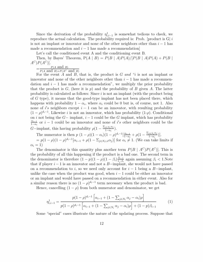
Example 1 Let n ≥ 9 and n be odd.15 Let Γ be as follows. Individual 1 has just 2links to 2 and 3. Divide the set {4, . . . , n} into two equal subsets, let 2 be connectedto all individuals in the first subset, each of whom have no other link. Similarly,let,individual 3 be connected to all agents in the second subset, each of whom haveno other link.

15See Figure 1 for the case n = 9.

18

Figure 1: Example 1

6

5

4

9

8

7

2 1 3

Assume that

δ ≥ max

(

4

n− 3,n− 5

n− 3

)

First, notice that if type G places his implant at 1 and all subsequent recommen-dations are accepted with probability one, then his payoff is 2δ + (n − 3)δ2 − c. Onthe other hand, if he places his implant at 2 or 3, then his payoff is (((n − 3)/2) +1)δ + δ2 + ((n− 3)/2)δ3 − c. The inequality δ ≥ n−5

n−3ensures that the first sum is at

least as large.Second, assume also that p and p̄ are such that the type B can put probability 1/2

on each of the nodes 2 and 3, and still make a credible recommendation in period 2.That is, the neighbors of 2 and 3 have to infer whether sites 2 and 3 have receiveda recommendation from the implant of type G placed at 1 in the previous period orwhether it is the type B implant who is speaking in period 2, having strategically keptsilent in period 1. A probability weight of β2 = β3 = 1/2 brings their updated beliefthat the recommendation is being passed on from 1 to the threshold p, given the initialparameter values.

Then, the following is an ODE. The type G puts his implant at 1 with probability1, the type B randomizes between 2 and 3 with equal probability. The type G implantspeaks immediately while the type B implant speaks in period 2. All recommendationsare accepted with probability one.

These constitute an equilibrium because if δ ≥ 4n−3

, then the type B implant has noincentive to deviate and place his implant at 1 - he gets δ2(n−3)/2−c in equilibrium,whereas he would get 2δ − c by placing his implant at 1. The response decisions areoptimal because updated beliefs are not below the threshold.

In general, ρ = 0 gives “less cover” for the B type to hide itself. It also creates

19

more zero-probability events, giving rise, for example, to a no-trade equilibrium, inwhich neither type of firm chooses to enter with an implant. If anyone does enterand recommends the product, it is believed to be a B type and no buyer buys.

How does a positive ρ impact on the possibility of optimal diffusion? Fix all otherparameters and the network structure Γ. Now, ρ influences the nature of equilibriumin two ways. First, the higher the value of ρ, the lower is the net gain from having animplant for both firm types. So, there will be some value of ρ̄ such that if ρ ≥ ρ̄,thenone or both types of firm F will refrain from employing an implant.

Second, the value of ρ influences the updating process according to equation 1.Suppose ρ changes. How does this affect η1i,i−1 for a fixed value of βi and distributionα? An increase in ρ makes it more likely that i− 1 is an innovator, but also makesit less likely that none of the other neighbors of i are innovators. These effects movein opposite directions and an unambiguous answer is difficult to provide.

5 The Line Network

In this section, we provide a discussion of a specific network structure - the line , inorder to illustrate the conditions required for complete and optimal diffusion equi-librium. Much of the intuition underlying the model can be obtained by analysingwhat happens in the case of the line. In particular, the importance of largeness foroptimal diffusion is perfectly illustrated by this network.

Assume, for simplicity, that n is odd, so that Assumption S is satisfied. So, let Γbe a line, with the sites ordered so that 1 and n are the end-points of the line havingdegree one, whilst all other sites have degree 2. Since n is odd, the unique medianm maximizes diffusion centrality.

We discuss informally the ODE type of equilibrium. A theorem and formal proofof our results on the line follow this informal discussion. We will conclude this sectionwith examples illustrating other types of CDE.

If (α, β) is to be an ODE, then the recommendation coming from m has tobe accepted with probability one. That is, m − 1 and m + 1 must accept anyrecommendation coming fromm with probability one. Since the bad type can alwaysmimic the Good type, this implies that wherever the bad implant is placed, herrecommendation must be accepted by two neighbors. Out-of-equilibrium, if an offeris rejected, the recommendation does not proceed farther along the path where thereis a rejection, though it might elsewhere. No player who has a subsequent move canobserve this deviation; all they can observe is that no recommendation reaches them,which occurs with positive probability along any path.

20

But, of course, βm 6= 1. For, if βm = 1, then from equation (1),

η1m−1,m − p = η1m+1,m − p = p[((1− ρ)− 1)(1− p)

p(1− ρ) + (1− p)] < 0,

and neither of m’s neighbors would buy the product after receiving a recommenda-tion from m, which is a contradiction. So, while the support of β can include m, itcannot coincide with {m}. Over what set of nodes can the bad type “distribute” β?The answer of course is that the support of β must be contained in those nodes whocan make “credible” recommendations to both their neighbors, since m’s recommen-dations should be credible. That is, it must be the set of nodes with effective degree2. Set

E2 ≡ N \ {1, m− 2, m− 1, m+ 1, m+ 2, n}

It is clear that 1 and n cannot be in E2 since they have only one neighbor. Althoughm − 2 and m + 2 have degree 2, notice that m − 1 (respectively m + 1) will notbelieve a single recommendation from m− 2 (respectively from m+ 2).16 Of course,m− 1 and m+1 cannot sell to m. Also, notice that if n < 9, then m will be the solemember of E2, and there will not be any ODE.

It is also clear when the bad type will want to use an implant when there is anODE. Let the implant be placed at i. Since i can be an innovator with probabilityρ (in which case he would buy the product anyway), the effective cost of an implantat i is

ρ+ c

The benefit is the additional probability that i− 1 and i+ 1 buy the product. Withprobability (1− ρ)2, neither is an innovator. With probability 2(1− ρ)ρ, one of thetwo is an innovator. Hence, the benefit is

2(1− ρ)2δ + 2(1− ρ)ρδ = 2δ(1− ρ)

So,the net gain of an implant for B is given by

2δ(1− ρ)− ρ− c

where c is the cost of an implant. So, B will use an implant if

c ≤ cB(δ, ρ) ≡ 2δ(1− ρ)− ρ

16Both m − 1 and m + 1 know that if the product is good, then m would have made a recom-mendation.

21

Not surprisingly, the higher the value of ρ, the lower is the expected gain fromemploying an implant.

Consider G. Let πG(δ, ρ) denote the profit of G in the absence of an implant, andπ̄G(δ, ρ) denote the profit of G if an implant is used.

Then, G will use an implant if

c ≤ cG(δ, ρ) ≡ π̄G(δ, ρ)− πG(δ, ρ)

The fact that the B-type implant’s recommendation has to be credible imposesan upper bound on the value of βi. The bound can be determined from equation 1.

It is now easy to describe what an ODE looks like when n ≥ 9 is odd, and thecost of an implant does not exceed c.

(i) The type G firm puts its implant at the median of the line with probabilityone.

(ii) The support of β is contained in E2, and the recommendation from each nodein the support is credible.

(iii) The implant (irrespective of type) “speaks” in period 1.Response decisions must support full diffusion - we spell this out in the proof of

the theorem.In the theorem below, we make a very mild assumption on out-of-equilibrium

beliefs to show that for ”large” networks, the only PBE is an ODE.Assumption D1. Let the sender of type t ∈ T choose to send a message m ∈ M.

Let the receiver respond with an action a from A. Consider the set of responses tothe message m that induces type t to weakly prefer to send the message m ratherthan the candidate equilibrium message m∗. Denote this set by At ⊆ A.If there is atype t′ who strictly prefers sending message m (to the equilibrium message) if theresponses are in At, then the belief of the receiver on receiving message m mustaccord probability 0 to type t.(See [3]).

The D1 refinement of sequential equilibrium essentially requires that if an out-of-equilibrium message is observed, the responder puts the entire weight of her updatedbeliefs on the set of types that gain maximally from the deviation. The attractiveproperties of this refinement in generic signaling games are examined in detail in [4]

Fix (ρ, p, p̄). The integer bounds specified in the theorem below are with respectto this vector of parameter values. We will also assume that Assumption S is satisfied.However, the proof makes it clear that this just simplifies the computation of thebounds - there will be no qualitative change in the result if Assumption S is notsatisfied.

22

Theorem 2 Suppose Assumption S holds. Then, there are integers n1, n2 such thatn2 ≥ n1 > 7 such that

(i) There is an ODE iff n ≥ n1.

(ii) Moreover, if D1 is satisfied and n ≥ n2, then the only PBE is an ODE.

We now give examples of other types of equilibria on the line. It follows thateither a different PBE exists along with an ODE or n is smaller than n1 .

Our first example is one where n = 7 so that an ODE does not exist, but a

CDE does exist. Recall that from equation 1, b1 ≡ ρ(1−ρ)p1−p

[

(1−p̄)p̄

]

is the probability

weight of the B-implant on i which ensures η1j,i = p̄ when αi = 0. That is, this isthe probability weight of the B-implant on i which makes neighbor j of i indifferentbetween accepting or rejecting a recommendation from i. Assume that

7b1 ≥ 1

Example 2 Let n = 7. then, the following is a CDE.

• α1 = 1.

• βi = b1 for i = 3, 4, 5, 6.

• βi = max(0, 1−4b1

3) for i = 1, 2, 7.

Any implant speaks in period 1. The response decisions are the following.(i) For each i 6= 7, only i + 1 accepts the recommendation of i and does so with

probability one in period 1.(ii) Node 6 accepts the recommendation from 7 in period 1.(iii) Node 1 + t accepts her left neighbor’s recommendation in period t > 1.So, each period 1 recommendation is accepted by exactly one node. In subsequent

periods, diffusion of the good product happens from left to right.Since the period 1 updated probability is exactly p̄ for recommendations coming

from i = 3, 4, 5, 6, it is an equilibrium response for i+ 1 to accept and i− 1 to rejectthe recommendation. The updated probability of recommendations coming from 1,2,7is either greater or equal to p̄. Noting that 1 will not accept any recommendationfrom 2 (since α1 = 1), the other response decisions are also optimal.

The G-implant achieves complete diffusion. Any deviation yields lower expectedpayoff since the product does not diffuse to the left. The B-implant gets one accep-tance. No deviation does better. Hence, this constitutes a CDE.

23

Since the G-implant locates at an extreme node, the set of possible nodes whichcan be the support of β includes nodes with effective degree one. This increase inpossibility allows a CDE to exist for n = 7. That is, ”small” networks which cannotsustain ODE can nevertheless sustain CDE.

The next example shows that a network size which allows ODE to exist can alsosustain CDE where the G-type does not locate at m. In fact, in the example below,m is not in the support of either α or β. The B-type implant gets two acceptancesin equilibrium and hence has no reason to deviate to m. The G-type implant wouldlike to deviate to m but recommendations are not accepted for reasons we explainbelow.

Example 3 Let n = 9, and

p(1− p̄)(1− ρ)

p̄(1− p)+ 2

ρ(1− ρ)p

1− p

[

(1− p̄)

p̄

]

≥ 1

Let

• α4 = 1, αi = 0 for all i 6= 4.

• β4 =p(1−p̄)(1−ρ)

p̄(1−p)

• β7 = β8 =1−β4

2≤ ρ(1−ρ)p

1−p

[

(1−p̄)p̄

]

• βi = 0 for all other i.

Response decisions are the following.(i) 4 does not accept any recommendation.(ii) Every other node accepts all other recommendations in period 1.17

Since α4 = 1, E2 = {7, 8}. Readers can check that β4 corresponds to βm fromthe previous theorem, while β7 = β8 does not exceed the probability weight that makesrecommendations just credible from nodes which are not in the support of α. So,these ensure that the response decisions of all nodes other than 4 are optimal.

What should 4 (if no implant is placed there) do if it receives a recommendationfrom 5, which is the median? Note that this is an out-of-equilibrium move if itcomes from an implant (though the type of player making the recommendation is notobservable). In equilibrium, it can only come from an innovator since 5 is not in the

17For t > 1, response decisions support complete diffusion. We do not specify these since theyplay no role.

24

support of either α or β. But, 4 ”knows” that if the product is good, then it shouldhave a G-implant. So, the recommendation cannot be from an innovator - it must befrom a deviant of either the G- or B-type. If D1 is not imposed, then 4 can assignthe belief that the recommendation is from the B-implant and hence not accept therecommendation. Given this, the G-type implant has no incentive to deviate to 5,which is the median.

Hence, the prescribed strategies constitute a PBE which is a CDE. Of course,there is also an ODE where α5 = 1 with the support of β being {2, 5, 8}.

6 Constraining both types of implant to speak in

the first period.

As a further simplification of the model, we could require that both the G and Bimplants must speak in the first period, with the innovators. This would imply thatany recommendation received in the second period would be considered to be passedon from a recommendation received in the previous period and therefore a signal of agood type. For the equilibria discussed in the last section and, for general networksin which the probability of acceptance is either 1 or 0 by any node, this restrictiondoes not affect the equilibria. In an ODE, even if the B type had the option to wait,he would not do so because a payoff of 2 is greater than one of 2δ.The G type, ofcourse, will not wait.

The restriction will have some bite if∑

i βi < 1, ( see the previous section for theline) for the set of nodes in the support of the B type’s random behavioral strategy.This means that B does not have enough nodes in the support of his mixed strategyto make the neighbors of these nodes indifferent between accepting and rejecting arecommendation. If the entire probability mass is distributed on these nodes, someneighbors will have p < p and will therefore reject the recommendation, even ifthey are myopic. In this case, the equilibrium (for ρ > 0) has to have the B typerandomize between entering with an implant or not. The residual probability has tobe on not entering. Any recommendation will be accepted with a probability thatmakes the B type’s expected payoff equal to c, the cost of the implant. The G typewill strictly prefer to enter with an implant because she will obtain payoffs afterthe first period as well, whilst the B type can only get payoffs from his immediateneighbors and not from their neighbors.

We can also see the effect of restricting both types to speak in the first period inthe example in Figure 1. Here the B types locate at the two nodes that are connectedto three leaves each, whilst the G type locates at the node that is connected to these

25

two nodes only. This will only work if the ρ provides enough “cover” for the B typeto put all his probability mass at these two nodes. If he were allowed to speak also inthe second period, he could also exploit the feature of equilibrium that the G type’srecommendation can be passed on to the leaves in the second period, thus reducingthe amount of probability mass associated with a first period recommendation. If Bis required to speak in the first period, a deviation by B to speaking in the secondperiod is infeasible. B can then locate at one of three nodes so as to make neighborsindifferent between accepting and rejecting and put the remaining probability mass,if any, on not entering. Acceptance and rejection probabilities can be adjusted tomake B indifferent between entering and not entering.

7 A Partial Characterization Result

In this section, we describe a sufficient condition for an ODE to exist, and then showthat this condition is necessary for certain types of network structures.

Throughout this section, we restrict our attention to networks satisfying Assump-tion S.18

Given m, partition nodes into sets S1, . . . , SK such that S1 is the set of nodesmaximizing d̄i, S2 is the set of nodes with the next highest value of d̄i, and so on.

Suppose that node i is in the support of β, and j ∈ N̄i. Whether j finds therecommendation credible or not depends on the degree of j since she does not re-ceive a recommendation from any neighbor other than i. Clearly, the larger thenumber of neighbors of j, the lower is the updated probability after receiving i’srecommendation.

For every node i, let ki be the site in N̄i that maximizes degree. Then,

η1ki,i ≤ η1j,i for all j ∈ N̄i

For each j ∈ N̄i, let βji be the value of βi which sets η1j,i = p̄j.

For each i, β̄i ≡ minj∈N̄i

βji (2)

So, if βi ≤ β̄i, all neighbors of i in N̄i find i’s recommendation credible.The next theorem identifies a sufficient condition for a network structure to sup-

port an ODE. It also shows that this is “almost” necessary. These conditions aresatisfied by the line, and so this theorem will include the line as a special case.

18This assumption results in somewhat more transparent results. In an earlier version, we didnot use this assumption here. That version is available from the authors.

26

Theorem 3 Suppose the cost of an implant is sufficiently low19 for both types of thefirm to use an implant. Then, an ODE exists if

∑

i∈S1

β̄i ≥ 1. (3)

Conversely, an ODE does not exist if m is critical, m ∈ S1 and equation 3 doesnot hold.20

Equation 3 is easy to interpret. If there are a sufficient number of nodes maxi-mizing effective degree, then an ODE is easy to support since the type B firm hasenough “space” to distribute his probability. Conversely, if an ODE is to exist, thenit must be possible for the type B firm to ensure that a recommendation from eachnode in the support of its mixed strategy is credible for |S1| neighbors.

Why is equation 3 not necessary without additional conditions? Suppose, thatαm = 1, but m /∈ S1, but say in S2. Also, assume that equation 3 does not hold. Itis possible then to have another equilibrium in which (i) the type B uses a mixedstrategy over nodes in S1∪S2, (ii) the probability of acceptance of recommendationscoming from nodes in S1 is adjusted below one so as to ensure that the expected payofffrom an implant located in S1 is the same as that from an implant in S2. However,the value of δ cannot be too high. If δ is high, then the low discounting may inducethe type B implant at some site in S1 to strategically postpone her recommendationto a later period. The freedom to distribute some probability weight over nodes inS2 may now help in ensuring existence of equilibrium. 21

If m ∈ S1 but is not critical, then there could be an equilibrium of the followingkind. The good product may diffuse throughout the network with probability oneeven if some neighbors of m who do not constitute critical links with m refuse m’srecommendations - the fact that some link mi is not critical obviously implies thatthere is some path from m to i not involving the link mi. An implication of thisis that the type B firm needs fewer customers in equilibrium. Now, suppose eachnode i ∈ S1 has one neighbor in N̄i(Γ) with very high degree, say hi, while theothers have relatively low degree. Then, one option for the type B firm is to put

19For the B type, given the network, this is the condition that the effective cost c+ ρ is less thanthe maximal effective degree. For the G type, the upper bound on c is harder to express explicitlybut it depends only on the total number of nodes, ρ and δ. Therefore, c is less than the minimumof these two upper bounds.

20Hence, equation 3 is necessary for the existence of an ODE in all trees satisfying AssumptionS and where m ∈ S1.

21An example of such an equilibrium is available in a previous version of the paper.

27

Figure 2: Example 4(Tree 1 )

5

4

7

6

2 1 3

probability weights β̃i > β̄i on each i such that all nodes in N̄i(Γ) except hi accepti’s recommendation.

The sufficiency condition in Theorem 3 is phrased in terms of effective degrees,and not in terms of “standard” network characteristics such as degree distribution ordiameter of the network. This is almost inevitable because the type B firm will chooseto place his implant at some node maximizing effective degree, and that latter doesnot easily translate into the familiar network characteristics. The following exampleshows that two networks with the same degree distribution can have quite differentproperties with respect to the existence of an ODE.

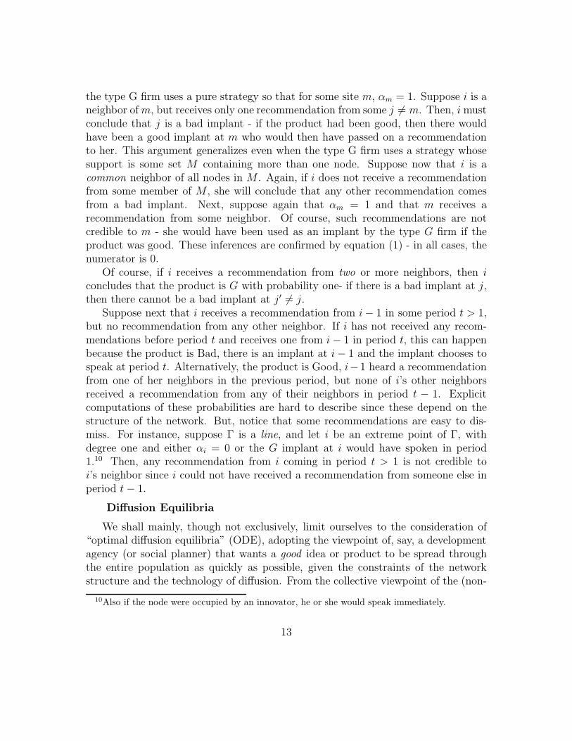
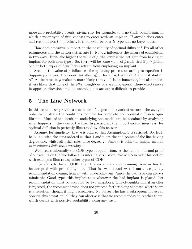
Example 4 In this example both networks are trees with the same degree distribu-tion, such that there is an ODE in one , but not in the other. Let n = 7.

Tree 1: Node 1 is connected to nodes 2 and 3; node 2 is connected to 4 and 5,while node 3 is connected to 6 and 7.

Tree 2: Node 1 is connected to 2,3,4; 4 is connected to 5 and 6, while 6 isconnected to 7.

Both trees have degree distribution (3, 3, 2, 1, 1, 1, 1). In tree 2, node 4 maximizesdiffusion centrality for all δ > 0. In tree 1, node 1 maximizes diffusion centrality forδ > 1/2.

Let δ > 1/2. Although both trees have the same degree distribution, the distribu-tion of effective degrees is not identical. In tree 1, the distribution of effective degreesis (2, 2, 2, 0, 0, 0, 0). To see this, check that nodes 1,2,3 all have effective degree 2,while the rest have effective degree 0. In tree 2, the distribution of effective degreesis (3, 2, 0, 0, 0, 0, 0). For some parameter values, it is possible to sustain an ODE intree 1, where α1 = 1, while the support of β is {1, 2, 3}. It is easy to see that noparameter values can sustain an ODE in tree 2.

28

Figure 3: Example 4(Tree 2 )

1

2

3

4

6

5

7

8 The Role of the Network Structure

In this section, we show that “dense” networks are not necessarily conducive forcomplete diffusion, a conclusion which is in stark contrast to the received wisdom inmodels where credibility is not an issue. We show that the complete network cannotsupport a CDE, while no network that contains a star encompassing all nodes cansupport an ODE.

In what follows, for any setM ⊂ N , and for any i /∈M , let N̄i(M) = Ni\∩j∈MNj ,and d̄i(M) = |N̄i|. The interpretation of N̄i(M) is that if M is the support of α,then N̄i(M) is the set of potential customers of i. Since individuals in ∩j∈MNj areconnected to all nodes in M , they will not accept any recommendation from a nodei /∈M .

Theorem 4 (i) If Γ is the complete network, then it cannot support a CDE.(ii)Suppose Γ contains a star as a subgraph. Then, Γ cannot support an ODE.

Under Assumption S, we can also place an upper bound on the degree of m.

Theorem 5 Let Assumption S hold, with m the unique node maximizing diffusioncentrality in Γ. Then, if Γ is to support an ODE, dm ≤ n−1

2.

Theorems 4 and 5 describe some network structures that cannot support an ODE.In particular, nodes maximizing diffusion centrality cannot be too well-connectedsince their connections tend to reduce the effective degree of those nodes which are“close” to them.

29

9 Extensions

We consider some possible extensions of the basic model.

9.1 Negative recommendations

We have assumed that “recommendations” can only be positive. However, one needsto consider negative recommendations as well if only to consider the robustness ofthe model. It is easy to check that Theorems 1, 4 and 5 continue to remain valid.

It also turns out that the possibility of negative recommendations will actuallysimplify calculations in one respect in that the probability calculations would notnow depend on the potential recipient’s degree. So, the analogue of equation 1 willnow be

η1i,i−1 =p[

αi−1 + (1−∑

j∈Niαj − αi)ρ

]

p[

αi−1 + (1−∑

j∈Niαj − αi)ρ

]

+ (1− p)βi−1

(4)

However, it would complicate expected payoff calculations for B, where a highdegree recipient of an implant’s (positive) recommendation would be more likely tohave countervailing negative information than one of low degree. Such a problemwould not arise for regular graphs, but the general issue is illustrated below.

So, suppose B places implants at i and j with some positive probability. Then,his expected payoff from i is

Ei =∑

k∈N̄i

(1− ρ)dk−1Pk

where Pk is the probability with which the offer is accepted by k. The updated belieffor all k ∈ N̄i(Γ) will now be the same - it will just depend on βi and not on thedegrees of k.

So, since Ei = Ej, we need∑

k∈N̄j

(1− ρ)dk−1Pk =∑

k∈N̄i

(1− ρ)dk−1Pk

The specification of a general sufficient condition is now more difficult because thederivation of the support of β is now more complicated. However, the qualitative re-sult that a larger network is more conducive for optimal diffusion remains unchangedfor the line and regular networks.

The possibility of negative recommendations may also help in sustaining optimaldiffusion, particularly in dense networks where nodes have high degree. This is

30

because the expected payoff of the type B firm will now be lower- and it will belower the larger are the degrees of different sites that can be recipients of implantrecommendations. So, the type B firm may simply not employ implants.

9.2 Multiple implants

If the firm can choose multiple implants, the qualitative features of the analysiswill be similar. Clearly it does not make sense for the multiple implants to haveoverlapping supports (for the firm’s randomized strategies). This suggests that forlarge networks, the firm will partition the networks in such a way as to have oneimplant randomly located (for B) in each element of the partition. If δ is close to 1and an ODE exists as above, there is very little incentive for G to incur the cost ofan additional implant, since this can only speed up the diffusion and the benefit fromthis might be low compared to the cost. Therefore, for low discounting, we wouldexpect to have several B implants but only one G implant. This suggests that the Bimplants would either have to rely on a relatively high ρ for credibility or speak onlyat sufficiently late time periods to mimic a message transmitted along the networkfrom a supposed good implant, which might be located some distance away.

9.3 The bad type’s probability of producing a good product.

We have assumed so far that Firm F knows its type, where type is identified withthe quality of the product that is produced. Let us redefine type as follows. Thetype G firm produces a good product with probability one, while type B produces agood product with small positive probability ǫ and the bad product with probability1− ǫ. Suppose as before that firm F knows its type in the modified sense.22

In this case, the following cases could arise (this is not an exhaustive description):(i) There is a unique node m maximizing diffusion centrality, which also maxi-

mizes degree centrality. In this case, an ODE will not exist. The reason is that bothG and B will care about speed of diffusion, though B will care less, and thereforeboth will prefer to locate at m rather than at any other node. As pointed out earlier,both types locating with probability 1 at m cannot be an equilibrium.

(ii) There is a unique node m maximizing diffusion centrality but it does notmaximize effective degree centrality. Now B will be better off not locating at m forε small enough. If he locates at a site that has effective degree at least 1 more than

22Alternatively, suppose type is identified with quality of the product as before, but consumerswho buy the bad quality product make a “mistake” with small probability - they make a positiverecommendation with probability ǫ.

31

m, he can get some additional payoff. If he locates at m, he loses at least 1 for sureand obtains some additional payoff depending on ε and δ. For ǫ small enough, thisis not a best response for B. In this case, the analysis from the firm’s point of viewwill not change from that discussed earlier in this paper. Hence, an ODE will existunder the same conditions as before.

10 Conclusions

In this paper, we have explored the implications for diffusion of a product or atechnology to a network of rational consumers and “innovators”, where the sellerof the product or technology has private information about its quality. Consumersare aware that firms may “seed” the network, and also know that both “good” and“bad” quality firms may do so. As a result, agents cannot take recommendationsfrom their social neighbors at face value - the credibility of recommendations hasto be evaluated with beliefs updated using Bayes’ Rule. Within this framework, weshow that a priori notions about what network structure is conducive to optimaldiffusion may be misleading. In particular, “small” networks and highly-connectedagents may actually impede the diffusion of the good product. The requirementof credibility of learning has bite; these results would not hold in a model withoutrationality. Also the entire structure of the network is important in determiningwhether optimal diffusion is possible or not, though the nodes with the highestdegree and those that maximize “diffusion centrality”, a notion of centrality thattakes into account whether an agent is connected to other agents who are themselvescentral, play special roles in the equilibrium pattern of implants and diffusion.

References

[1] Bala, V. and S. Goyal, (1998) “Learning from Neighbours”, Review of EconomicStudies, 65, 3, 595-621

[2] Chatterjee, K. and S.Hong Xu, (2004), ‘Technology Diffusion by Learning fromNeighbours’, Adv. in Appl. Probab., 36, 2, 355–376

[3] Cho, I-K. and D.M. Kreps, (1987), ”Signaling Games and Stable Equilibria”.TheQuarterly Journal of Economics, 102(2):179-221, 1987.

32

[4] Cho, I-K and J. Sobel (1990), “Strategic Stability and Uniqueness in SignalingGames”, Journal of Economic Theory, 50, 381-413.

[5] Coleman, J.S., E.Katz and H.Menzel (1966), Medical Innovation: A DiffusionStudy, Indianopolis, Indiana, Bobbs-Merrill.

[6] Conley, T.G., and C. Udry, (2010) “Learning About a New Technology: Pineap-ple in Ghana”, American Economic Review, 100, 1, 35-69.

[7] Draief, Moez and Laurent Massoulie (2010), Epidemics and Rumours in Com-plex Networks, London Mathematical Society Lecture Notes no. 369, CambridgeUniversity Press, Cambridge, UK.

[8] Durrett, Rick T. (2007), Random Graph Dynamics, Cambridge University Press,New York and Cambridge.

[9] Ellison, Glenn, (1993), “Learning, Local Interaction and Coordination”, Econo-metrica, 71, 1047-1071.

[10] Ellison, Glenn and Drew Fudenberg(1993), “Rules of Thumb for Social Learn-ing”, Journal of Political Economy, 101, 612-644.

[11] Ellison, Glenn and Drew Fudenberg(1995), “Word-of-mouth Communicationand Social Learning”, Quarterly Journal of Economics, 109, 93-125.

[12] Foster, A.D. and M.Rosenzweig (1995), “Learning by Doing and Learning fromOthers: Human Capital and Technological Change in Agriculture”, Journal ofPolitical Economy, 103, 1176-1209.

[13] Galeotti, A. and S. Goyal, (2009), “Influencing the Influencers: a Theory ofStrategic Diffusion”, RAND Journal of Economics, 40, 3, 509-532.

[14] Goyal, S., (2005), “Learning in Networks”, in G.Demange and M.Wooders (ed)Group Formation in Economics, Cambridge, Cambridge University Press.

[15] Goyal, S. and A. Vigier (2010), “Robust Networks”, mimeo, University of Cam-bridge, Faculty of Economics.

[16] Guardian newspaper, The (2013), “India farmers think big but grow micro toenrich their soil,” March 13.

[17] Jackson, M., (2008), Social and Economic Networks, Princeton University Press,Princeton, New Jersey, USA.

33

[18] Jackson, M. and L. Yaariv (2010), “Diffusion, Strategic Interaction and So-cial Structure”, to be published in Handbook of Social Economics, edited byJ.Benhabib, A.Bisin and M. Jackson.

[19] Kempe, D., Kleinberg, J., and Tardos, E. (2003), “Maximizing the Spread ofInfluence in a Social Network”, Proceeding of the Ninth ACM SIGKDD Inter-national Conference on Knowledge Discovery and Data Mining.

[20] Leskovec, J., Adamic, L.A. and Huberman B.A. (2007), “The Dynamics of ViralMarketing”, ACM Transactions on the Web 1, articl 5.

[21] Munshi, K., (2004), “Social Learning in a Heterogeneous Population: Technol-ogy Diffusion in the Indian Green Revolution,” Journal of Development Eco-nomics, 73 ,1, 185-213.

[22] Rogers, E. (2003), Diffusion of Innovations, New York: Free Press.

[23] Richardson,M., and P.Domingos (2002)“Mining Knowledge-Sharing and Sitesfor Viral Marketing”, Proceeding of the Eighth ACM SIGKDD InternationalConference on Knowledge Discovery and Data Mining.

[24] Silverman, G (2001), The Secrets of Word-of-Mouth Marketing: How to TriggerExponential Sales through Runaway Word of Mouth, New York, Amacom books.

[25] Walker, Rob, (2004) “The Hidden (in Plain Sight) Persuaders”, The New YorkTimes Sunday Magazine, December 5.

[26] Young, H. Peyton (2009), “Innovation Diffusion in Heterogeneous Populations;Contagion, Social Influence and Social Learning”, American Economic Review,99, 1899-1924.

11 Appendix A : Proof of Theorems

Here, we provide proofs of all the results in the text.

Proof of Theorem 1

Proof.

(i) Suppose (α, β) is a CDE. Let M be the support of α.ny node i knows thatif the product is good, then it should receive a recommendation in period 1 fromsome node in M . So, a recommendation from nodes outside M are not credible.

34

Hence, the support of β must be a subset of M . But, then equation 1 shows thatthe updated probability will be less than p̄. This proves (i).

(ii) Let M be the set of nodes maximizing diffusion centrality. If an ODE exists,then the support of α is contained in M . For simplicity, assume it is M .

Let m ∈M . If m is critical, then all of m’s neighbors must accept m’s recommen-dations. If some neighbor j does not accept m’s recommendation with probabilityone, then the criticality of m implies that the good product will not diffuse to somesegment of the network. Suppose βi > 0, where i /∈ M . Then, the implant at i can-not make its recommendation in period 1 since recommendations from nodes otherthan those in M are not credible in period 1. So, the payoff to the implant at i is atmost δdi < dm, since m maximizes effective degree. So, if the bad implant could belocated at m, it would get a higher payoff. This implies that the support of β shouldbe contained in M . But, then the updated probability at some m ∈ M would beless than p̄. This shows that the type B firm does not have an equilibrium strategythat sustains optimal diffusion.

Proof of Theorem 2

Proof.

(i) From our informal discussion of an ODE, it is clear that an ODE exists iffαm = 1, and

β̄i ≥ βi for i ∈ E2 (5)∑

i∈E2

β̄i ≥ 1 (6)

where E2 is the set of nodes which have effective degree two, and β̄i is the upperbound on βi. It follows that n ≥ 9 since otherwise E2 = ∅ when αm = 1 at themedian m.

Using equation 1, these are given by

β̄m =p(1− p̄)(1− ρ)

p̄(1− p), and for i 6= m, β̄i =

ρ(1− ρ)p

1− p

[

(1− p̄)

p̄

]

Let n1 be the smallest value of n such that

1− β̄mn− 7

≤ρ(1− ρ)p

1− p

[

(1− p̄)

p̄

]

(7)

So, there is no probability distribution β satisfying equations ??, 5 iff n < n1.This follows because the best the B-type implant can do to economize on the number

35

of nodes in the support of β is to assign β̄m to m and equal weight to all other nodesin E2.

This shows why there is no ODE if n < n1.Now, suppose n ≥ n1. Then, the following is an ODE.

(i) αm = 1.

(ii βm = β̄m ≡ p(1−p̄)(1−ρ)p̄(1−p)

(iii) βi =1−βm

n−7≤ ρ(1−ρ)p

1−p

[

(1−p̄)p̄

]

for all i ∈ E2 \ {m}.

(iii) βi = 0 for all i /∈ E2.

Moreover, the implant (irrespective of type) “speaks” in period 1.To complete the description of the equilibrium, we define the responses of all

nodes.First, all nodes accept recommendations received in period 1 with probability

one.In subsequent periods t > 1, a site i < m accepts a recommendation from i + 1

with probability one if the equilibrium response of i+1 was to accept the recommen-dation from i+ 2 in period t− 1. Similarly, a site i > m accepts a recommendationfrom i − 1 if the equilibrium response of i − 1 was to accept the recommendationfrom i− 2 in period t− 1.

Clearly, the Good product diffuses throughout the network, while the Bad prod-uct is bought by all innovators and the immediate neighbors of the B-type implant.

In order to see that these constitute a PBE, notice that after node i receives arecommendation from neighbor j in period t, ηti,j ≥ p̄. Hence, the response decision(of buying) of i is optimal.

The G-type implant does not want to deviate from αm = 1. This follows bynoting that type G cannot be indifferent between m and any other site. At m, theimplant will obtain an expected payoff of δ.2 + δ2.2+ .... for m− 1 terms. At m− k,say, the payoff will be δ.2 + δ2.2 + ...δt2 for m − k − 1 terms and δm−k.1 + .. foran additional 2k terms, thus taking m + k − 1 periods to diffuse completely ratherthan m− 1 periods, if the good implant locates at m.23 Thus the speed of diffusionis higher by locating at m, since there are two new buyers in each period for everyperiod the diffusion continues, whilst at m − k, there is only one buyer for everyperiod after k − 1.

23This calculation does not take ρ into account, but it is obvious this wouldn’t change the rankingbecause sites are independently innovators or non-innovators

36

The B-type implant has no incentive to deviate because at each node whereβi > 0, node i’s recommendation is accepted by both neighbors of i. Since the B-type good will be recommended only by the implant, this is the best that the B-typecan do.

Finally, we need to check whether the response decisions are optimal. Notethat since βi ≤ β̄i at all nodes, η1j,i ≥ p̄ for both neighbors j of i. Hence, it isoptimal for each j to accept any recommendation received in period 1. Since anyrecommendation received in period t > 1 must be coming from a node who has triedthe product in period t− 1 and found it to be good, acceptance of recommendationsreceived in period t > 1 is also optimal.

In this equilibrium, a message fromm in period 2 would be an event of probability0. To check that neither type wants to deviate, we have to consider out-of-equilibriumbeliefs, but all beliefs about the type sustain this equilibrium. The m implant’srecommendation is accepted with probability 1 in the first period, so discountingmakes it sub-optimal to wait, no matter what the belief.

This completes the proof of (i).

(ii) Suppose D1 is satisfied and there is a PBE (α, β) which is not an ODE.

Case 1: Suppose first that the PBE is a CDE.Of course, αm = 0. For if αm > 0, then the CDE would in fact be an ODE,

contradicting our assumption. In fact, αi = 0 for any interior node i. For supposeαi > 0 where i 6= 1, n. Since this is a CDE by assumption, both of i’s neighboursaccept i’s recommendation. So, the B-implant must also get two acceptances -otherwise the B-implant would deviate to i. If βm > 0, then the G- implant woulddeviate to m. This follows because m + 1 and m − 1 accept the recommendationcoming from m. Then, in period 2, m − 1’s and m + 1’s recommendations mustbe accepted by their neighbours. Continuing this chain of argument, the G-implantimproves payoff by achieving complete diffusion in the fastest possible time- thisjustifies the deviation by the G implant.

Hence, βm = 0. Now, suppose the G-implant deviates to m. When m makesa recommendation, either both m − 1 and m + 1 believe that m is an innovator,and accept the recommendation. Alternatively, one of them, say m − 1 concludesthat this is an out-of equilibrium move by an implant. This happens if αm−1 = 1 orαm−2 = 1. But, since the B-implant already gets two acceptances, it has no strictincentive to deviate to m even if both neighbors accept m′s recommendation (and anincentive not to deviate if this is not the case). On the other hand, the G-implant bygetting its recommendation accepted would achieve complete diffusion in the fastestpossible time, and so would strictly prefer to deviate if m′s recommendation was

37

accepted with probability 1. That is, the deviation from equilibrium is more likelyto have come from the G-implant. So, applying D1, m−1 must conclude that eitherm is an innovator or the G-implant has deviated to m. In either case, m− 1 acceptsthe recommendation and then recommends the good in the next period, if he findsit good. Continuing this argument, there must be complete diffusion from m oncethe G implant deviates. This again justifies the deviation.

So, the support of α is restricted to 1, n.Claim 1 If i ∈ E2, then βi > 0.Suppose the claim is not true. Then, any recommendation from i must be coming

from an innovator.24 Take any j 6= i such that βj > 0. Then, both j − 1 and j + 1accept j’s recommendation with probability one - otherwise the B-type would shift hisimplant to i where he gets two acceptances. This also implies that the B-type implantmakes a recommendation with probability one in period 1 itself since postponing arecommendation to period 2 does strictly worse given δ < 1.

Hence, any recommendation in period 2 signals that the product is good. But,then the G-type will deviate to i since node i’s recommendations will be accepted byi− 1, i+ 1 in period 1, i+ 1 and i− 1’s recommendations will be accepted in period2, and so on. This will be a profitable deviation since complete diffusion from aninterior node is faster than complete diffusion from an extreme node.

Hence, this establishes the claim.

Claim 2 : If i ∈ E2 is an interior node, then recommendations from i are acceptedwith probability γ such that 0 < γ < 1.

We know from Claim 1 that βi > 0. So, γ > 0. Suppose γ = 1. Then, theB-implant does not make a recommendation in period 2. From what we have saidin the proof of claim 1, this will imply that the G-type has a profitable deviation.Hence, γ < 1.

So, every node i ∈ E2 is in the support of β and a recommendation from i isaccepted with probability less than one. The latter means that the updated proba-bility is exactly p̄. From equation 1, this implies that βi = b > 0 for some b. But, forsome i ∈ E2, βi ≤ 1/k where k = |E2|. Since k ≥ n− 6, there is n′ such that βi < bfor all n ≥ n′. But, then η1j,i > p̄ where j is a neighbor of i. So, both neighbors of iaccept i’s recommendation with probability one. This contradiction establishes theproof of (ii) in Case 1.

Case 2: Suppose the PBE is not a CDE.Again, it must be the case that the recommendation of the B-implant is not

accepted with probability one by the 2 neighbors. From arguments in Claims 1 and

24Note that out-of-equilibrium beliefs are not involved when i ∈ E2.

38

2 in Case 1, it follows that for large enough n, this is not possible.This concludes the proof.

Proof of Theorem 3

Proof. Suppose equation 3 is satisfied. Let αm = 1 be the strategy employed by thegood type, and choose β such that

βi ≤ β̄i for all i ∈ S1

andβi = 0 if i /∈ S1

The response strategies are straightforward. All sites accept all recommendations inall periods.

It is easy to check that these strategies constitute a PBE. Clearly, the type Gfirm has no incentive to deviate since her implant is at the site maximizing diffusioncentrality and recommendations are accepted with probability one. Similarly, thetype B firm has no incentive to deviate since she obtains a payoff of d̄1−c, conditionalon no innovators in N̄1. Clearly, no other site can yield a higher payoff. The responsedecisions are optimal because (i) any recommendation coming from a site not in theunion of the supports of α and β must be coming from an innovator, and (ii) theupdated belief of any i after receiving a recommendation from a potential implant isat least as large as the threshold value p̄.

Consider now the necessity of this condition. First, the type G firm must bechoosing an αm = 1 in any ODE. Since m is critical in Γ, all neighbors of m mustaccept a recommendation from m with probability one in an ODE. So, the type Bfirm by placing her implant atm can obtain a payoff of |S1|−c. Hence, in equilibrium,the support of β must be contained in S1. Moreover, if βi > 0, every member ofN̄i(Γ) has to accept the recommendation of i. Hence, the maximum probabilityweight that the type B firm can put on i cannot exceed β̄i. This is not possible ifequation 3 does not hold.

Proof of Theorem 4

Proof. (i) The proof is almost identical to that of part (i) of theorem 1. Let Γ bethe complete network, and (α, β) be any PBE. If M is the support of α, then any iwill only accept a recommendation from some j ∈ M . This means the support of βmust also be in M . But, this will mean that the updated probability of any node inthe support of β is less than p̄. This shows that there cannot be complete diffusion.

(ii) Let M = {i ∈ N |di(Γ) = n− 1}. If Γ contains a star, this set is non-empty.Then, all members ofM maximize diffusion centrality. If an ODE exists, the supportof α is some M ′ ⊆ M . Take any site i /∈ M ′. Then, d̄i(M

′) = 0 since any site j 6= i

39

is connected to all nodes in M ′. So, the support of β is also M ′. Then, it followsfrom equation 1 that

η1j,i ≤ p < p̄

So, no neighbor of the bad implant at i buys the product after receiving a recom-mendation from i. Since the bad type is indifferent between all sites in the supportof β, no site in the support of β can get her recommendation accepted. This impliesthat only the good type employs an implant. However, this cannot be an equilibriumsince the bad type would then deviate and place an implant at some site in M ′.

Proof of Theorem 5

Proof. Let Γ support an ODE, and let dm = k. Then, for all i 6= m, d̄i ≤ n− k− 1.Suppose dm > d̄i for all i 6= m. Then the bad type would prefer to put her implantat m since recommendations from m are accepted with probability one. But, ifβm = 1, then η1m,j < p < p̄ and this is not consistent with m’s recommendationsbeing accepted. Hence, dm = k ≤ d̄i ≤ n − k − 1 for some i 6= m. This impliesdm ≤ n−1

2.

12 Appendix B: Example on diffusion and decay

centrality

In this appendix, we illustrate the difference between diffusion and decay centralityfor two networks with two hubs. The second network is obtained from the first bydeleting a node. The maximization for different values of ρ is done numerically, bygenerating different configurations of innovators for each value of ρ and comparing theaverage performance (across configurations) of each node in the network in achievingcomplete diffusion.

Prior to presenting the numerical calculation for these two networks, we illustratethe nature of the concept of diffusion centrality by considering the following example.Suppose we have a line of four nodes, labelled 1, 2, 3 and 4. We set ρ = .2 (recall thisis the probability that any given node is an innovator) and consider the “diffusioncentrality” measures for nodes 1 and 3. (That is we assume an implant is placed at 1or 3 and calculate the appropriately discounted time for the innovation to diffuse inthe whole network.) Thus, if there is one innovator placed at node 4, an event thathas probability (.2)(.8)3 of happening, if the implant is placed at node 1 then nodes1 and 4 will know of the product immediately and 2 and 3 the following period,giving a total discounted time to diffuse of 2+2δ. Denoting by ‘0’ the absence of aninnovator and by ‘1’, the presence of one, we can construct the following table:

40

Configuration Prob 1 30000 (.8)4 1+δ + δ2 + δ3 1+2δ + δ2

0001 (.2)(.8)3 2+2δ 2+δ + δ2

0010 (.2)(.8)3 2+2δ 1+2δ + δ2

0100 (.2)(.8)3 2+δ + δ2 2+2δ1000 (.2)(.8)3 1+δ + δ2 + δ3 2+2δ0011 (.2)2(.8)2 3+δ 2+δ + δ2

0101 (.2)2(.8)2 3+δ 3+δ1001 (.2)2(.8)2 2+2δ 3+δ0110 (.2)2(.8)2 3+δ 2+2δ1100 (.2)2(.8)2 2+δ + δ2 3+δ1010 (.2)2(.8)2 2+2δ 2+2δ

1110 (.2)3 (.8) 3+δ 3+δ1101 (.2)3 (.8) 3+δ 41011 (.2)3 (.8) 3+δ 3+δ0111 (.2)3 (.8) 4 3+δ1111 (.2)3 (.8) 4 4

The diffusion centrality of node 1 can be found by multiplying the numbers incolumns 2 and 3 and adding for all rows and likewise, columns 2 and 4 for thecentrality measure of node 3.

The difference in the centrality measures for 3 and 1 can be calculated to be

(.8)4(δ − δ2) + (.2)(.8)3(2δ − δ2 − δ3) (8)

> 0. (9)

Thus node 3 is more central than node 1, which is not a surprising result.The numerical example is described in the following pages.

41

Setting: delta=0.8. Simulation for 3000 times

Source node Decay Centralityrho=0 rho=0.1 rho=0.3 rho=0.5 rho=0.7 rho=0.9

1 5.58 5.58 6.43 7.30 7.66 7.82 7.962 5.58 5.58 6.43 7.30 7.66 7.82 7.963 5.58 5.58 6.43 7.30 7.66 7.82 7.964 5.58 5.58 6.43 7.30 7.66 7.82 7.965 6.18 6.18 6.85 7.47 7.72 7.84 7.966 6.08 6.08 6.78 7.41 7.68 7.82 7.967 5.89 5.89 6.82 7.65 7.92 7.99 8.008 4.87 4.87 6.06 7.20 7.64 7.82 7.969 4.87 4.87 6.06 7.19 7.64 7.82 7.96

10 4.87 4.87 6.05 7.20 7.64 7.82 7.96

Diffusion Centrality

��

�� ��

�� ��

�� ��

�

�

���

Setting: delta=0.8. Simulation for 3000 times

Source node Decay Centralityrho=0 rho=0.1 rho=0.3 rho=0.5 rho=0.7 rho=0.9

2 4.78 4.7808 5.6101 6.4510 6.8428 7.0267 7.15163 4.78 4.7808 5.6092 6.4560 6.8430 7.0260 7.15144 4.78 4.7808 5.6112 6.4571 6.8414 7.0243 7.15155 5.38 5.3760 6.0375 6.6428 6.9119 7.0441 7.15316 5.44 5.4400 6.0240 6.5843 6.8624 7.0251 7.15127 5.38 5.3760 6.1078 6.8260 7.0890 7.1811 7.19938 4.46 4.4608 5.3778 6.3499 6.8014 7.0171 7.15119 4.46 4.4608 5.3777 6.3477 6.8024 7.0174 7.1511

10 4.46 4.4608 5.3809 6.3536 6.8022 7.0174 7.1511

Diffusion Centrality

2 5

3 4

6 7

8

9

10