Creating Depth Maps from

Monocular and Stereoscopic Images

By: Ben Bodner, Jessica Coulston

Advisor: Ricardo Figueroa

Revision Date: May 28, 2012

Submitted in partial fulfillment of the requirements forthe BS degree in the School of Film and AnimationRochester Institute of Technology, Rochester, NY

Copyright, Ben Bodner and Jessica Coulston 2012

0.1 Abstract

The removal of certain portions of an image based on content is known as keying and is an impor-tant component of most digital effects work in the Motion Picture Industry. The two algorithmsproposed here determine the depth of objects in an image, creating a channel with depth infor-mation at every pixel that can be used to key out portions of the image based on their distancefrom the camera. Keying from depth information reduces the amount of preparation necessaryfor shooting as compared to traditional chroma keying and has a wider range of uses than lumakeying. The use of an accurate depth channel would also allow for insertion of computer generated(CG) content into live action scenes without having to manually select what portions of the sceneshould occlude the CG content. One algorithm produces depth channels from stereoscopic pairsof images, captured by a dual-camera rig designed for shooting 3D movies, and the other uses sin-gle monocular images. The monocular algorithm was ultimately unsuccessful because of problemswith the machine learning implementation but the method still retains merit for its simplicity. Thestereoscopic implementation found accurate depth in many cases and had several clear advantagesover chroma keying, but still had a lot of errors in depth estimation. The implementation hassignificant room for improvement.

0.2 Introduction

The most common forms of keying are chroma keying, which removes pixels based on color, andluma keying, which removes pixels based on luminance. Chroma keying typically requires the use ofa green screen background, along with a significant amount of lighting expertise and planning. Theuse of chroma keying also limits available colors for foreground objects, in order to avoid unwantedremoval of object surfaces. Luma keying is limited to usage on very bright or very dark portionsof an image, and is typically used for sky replacement.

The goal of the project was to create depth maps from both two-dimensional (2D) and three-dimensional (3D) captured images for the purpose of depth keying. Depth keying, unlike chromakeying, allows the user to capture an image anywhere, not just in front of a green screen, whichmakes lighting and set composition much less limited. It also has the possibility of eliminatingcommon problems like fringing and spill.

This paper includes a detailed analysis and discussion of implementation of one approach todepth map creation for both 2D and 3D. Many available methods were assessed and the mostpromising for each capture type were chosen for implementation. The depth keys have been assessedbased on the accuracy of depth information and quality of key as compared to light detection andranging (LIDAR).

0.3 Background

A significant amount of research and documentation exists on creating depth maps from stereoimage pairs. The process typically involves identifying matching pixels between the two imagesand using their disparity in combination with the cameras’ orientations to find depth. It is alsonecessary to determine which regions of one image do not have a matching region in the otherimage, due to the differing perspectives of the cameras, and determine how to interpolate depthinformation in these areas.

1

Most methods of creating depth maps from single 2D images rely on auxiliary devices to eitherdetermine depth independent from the camera or to add information to the scene to be used tohelp determine depth after image processing. For instance, one method analyzes the frequency ofa uniform static stripe pattern projected onto a scene to create a depth map.

The monocular method discussed here is ideal because it does not require an auxiliary device,and relies on traditional monocular image capture alone. This method analyzes variations in tex-ture across the image and how those textures are affected by scaling along with comparison of otherfeatures in the image.

0.4 Theory and Method

0.4.1 Depth Maps from Stereoscopic Capture

To create a depth map from a stereoscopic image pair, each pixel in one image must be matched tothe corresponding pixel in the other image. Each point in the scene should have a correspondingpixel from both cameras, except in cases where a pixel has imaged scene content that is occludedin the other image. Because the two cameras used to record the scene were arranged horizontally,corresponding pixels will only differ in location horizontally and not vertically, limiting the searchfor a matching pixel to a single line of pixels in the image, called a scan line.

To search for the corresponding pixels from both cameras, an area of pixels, called an imageblock, is centered on the pixel under scrutiny in the first image and then compared to imageblocks in the second image. The comparison is done using the luminance version of the images,and cross-correlating image blocks along the same scan line. The horizontal distance between twoimage blocks with high correlation is the disparity between the two blocks. When looking at thecorrelations between one block in the first image and the blocks on the same scan line in the secondimage, there will likely be multiple cases of high correlation. To narrow down which correlationactually represents matching image blocks, it must be considered that objects have low variationsin disparity across their surface, but large changes in disparity at their edges. Neighboring blocksin the first image should, in most cases, represent different portions of the same object in the scene,and thus neighbors should have approximately the same disparity, determined by their horizontaldistance from highly correlated blocks in the second image. So while one block in the first imagemay have a high correlation with multiple blocks in the second image and thus more than oneprobable disparity value, all neighboring blocks representing the same object should have oneprobable disparity value in common.

Figure 1 shows how the disparity of continuous objects can be identified, with the horizontal axisrepresenting horizontal image block location in the first image and the vertical axis representing thedisparity (the horizontal distance to the image block in the second image), with bright areas havinghigh correlation between the two image blocks. Although every single block from the first imagehas a high correlation to multiple blocks in the second image, bright horizontal lines form on thegraph where there is a common probable disparity between neighbors, representing a continuousobject in the scene [1].

2

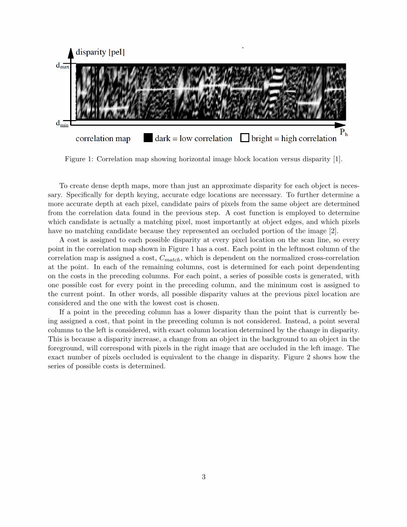
Figure 1: Correlation map showing horizontal image block location versus disparity [1].

To create dense depth maps, more than just an approximate disparity for each object is neces-sary. Specifically for depth keying, accurate edge locations are necessary. To further determine amore accurate depth at each pixel, candidate pairs of pixels from the same object are determinedfrom the correlation data found in the previous step. A cost function is employed to determinewhich candidate is actually a matching pixel, most importantly at object edges, and which pixelshave no matching candidate because they represented an occluded portion of the image [2].

A cost is assigned to each possible disparity at every pixel location on the scan line, so everypoint in the correlation map shown in Figure 1 has a cost. Each point in the leftmost column of thecorrelation map is assigned a cost, Cmatch, which is dependent on the normalized cross-correlationat the point. In each of the remaining columns, cost is determined for each point dependentingon the costs in the preceding columns. For each point, a series of possible costs is generated, withone possible cost for every point in the preceding column, and the minimum cost is assigned tothe current point. In other words, all possible disparity values at the previous pixel location areconsidered and the one with the lowest cost is chosen.

If a point in the preceding column has a lower disparity than the point that is currently be-ing assigned a cost, that point in the preceding column is not considered. Instead, a point severalcolumns to the left is considered, with exact column location determined by the change in disparity.This is because a disparity increase, a change from an object in the background to an object in theforeground, will correspond with pixels in the right image that are occluded in the left image. Theexact number of pixels occluded is equivalent to the change in disparity. Figure 2 shows how theseries of possible costs is determined.

3

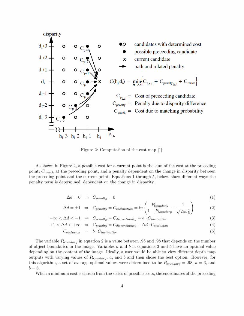
Figure 2: Computation of the cost map [1].

As shown in Figure 2, a possible cost for a current point is the sum of the cost at the precedingpoint, Cmatch at the preceding point, and a penalty dependent on the change in disparity betweenthe preceding point and the current point. Equations 1 through 5, below, show different ways thepenalty term is determined, dependent on the change in disparity.

∆d = 0 ⇒ Cpenalty = 0 (1)

∆d = ±1 ⇒ Cpenalty = Cinclination = ln

(Pboundary

1− Pboundary· 1√

2πσ2n

)(2)

−∞ < ∆d < −1 ⇒ Cpenalty = Cdiscontinuity = a · Cinclination (3)

+1 < ∆d < +∞ ⇒ Cpenalty = Cdiscontinuity + ∆d · Cocclusion (4)

Cocclusion = b · Cinclination (5)

The variable Pboundary in equation 2 is a value between .95 and .98 that depends on the numberof object boundaries in the image. Variables a and b in equations 3 and 5 have an optimal valuedepending on the content of the image. Ideally, a user would be able to view different depth mapoutputs with varying values of Pboundary, a, and b and then chose the best option. However, forthis algorithm, a set of average optimal values were determined to be Pboundary = .98, a = 6, andb = 8.

When a minimum cost is chosen from the series of possible costs, the coordinates of the preceding

4

point that was used in determining the cost are stored at the current point, along with the minimumcost that was chosen. When costs have been determined for all points in the correlation map, acandidate from each column is determined to be the correct disparity, so that every pixel location isassigned a disparity value. First, the point with the lowest cost in the last column of the correlationmap is assigned as the disparity value for the rightmost pixel, and the location that was storedat that cost is used to find the correct disparity in the second to last column. From there, thelocation stored at each disparity chosen is used to find the preceding correct disparity. This way, adisparity value is determined for every pixel location in the line, except where there was an increasein disparity and a corresponding occlusion.

The process of finding a correlation map for a row of pixels and then determining the correctdisparities from that map using the cost function is repeated for every row in the image, so that adisparity value is found for every pixel except where there is an occlusion. Along with the gaps indisparity due to occlusion, the resulting disparity map has other inaccuracies. Foreground objectsare expanded in all directions an amount dependent on the block size used in finding normalizedcross-correlation. Errors in determining correct disparity with the cost function can lead to falsechanges in disparity. To correct for these issues, the disparity map is compared with the luminancemap of the original image. Edge detection is used to find an edge map of both the disparity andluminance images. A line is drawn from each point in the disparity edge map to its nearest neighborin the luminance edge map. If that line is shorter than a maximum distance dependent on the blocksize used to find the correlation map, all pixels in the disparity map along that line are changed toa value equal to the disparity, on the side of the disparity edge opposite the nearest neighbor.

This disparity correction has the effect of shrinking foreground objects to their proper size andreplacing disparity gaps at occlusions, because disparity edges will be located outside luminanceedges, and all values between the edges will be changed to the disparity of the background object.Figure 3 shows the correction process, where ‘a’ is a point on the disparity edge map and ‘b’ is itsnearest neighbor in the luminance edge map. All pixels on the line between them in the disparityimage are changed to the disparity value at the pixel adjacent to ‘a’ in the direction opposite ofthe line.

5

Figure 3: Process of disparity correction.

Once corresponding pixel locations have been identified between the stereoscopic image pair, thedepth of the point in the scene represented by each pair of pixels can be determined geometricallyusing the disparity between corresponding pixels and the relative orientation and position of thecameras. Figure 4 shows the components necessary to determine depth. C is the optical center ofthe camera. A is a unit vector in the direction of the optical axis of the camera. H and V are unitvectors in the direction of the horizontal and vertical components of the image plane, respectively.f is the focal length of the cameras, so −f ∗A is a vector from C to the center of the image plane[3].

6

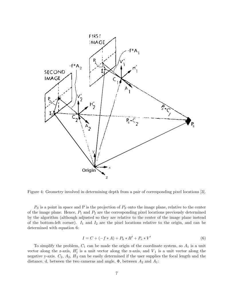
Figure 4: Geometry involved in determining depth from a pair of corresponding pixel locations [3].

PS is a point in space and P is the projection of PS onto the image plane, relative to the centerof the image plane. Hence, P1 and P2 are the corresponding pixel locations previously determinedby the algorithm (although adjusted so they are relative to the center of the image plane insteadof the bottom-left corner). I1 and I2 are the pixel locations relative to the origin, and can bedetermined with equation 6:

I = C + (−f ∗A) + Ph ∗H ′ + Pv ∗ V ′ (6)

To simplify the problem, C1 can be made the origin of the coordinate system, so A1 is a unitvector along the z-axis, H ′1 is a unit vector along the x-axis, and V 1 is a unit vector along thenegative y-axis. C2, A2, H2 can be easily determined if the user supplies the focal length and thedistance, d, between the two cameras and angle, Φ, between A2 and A1:

7

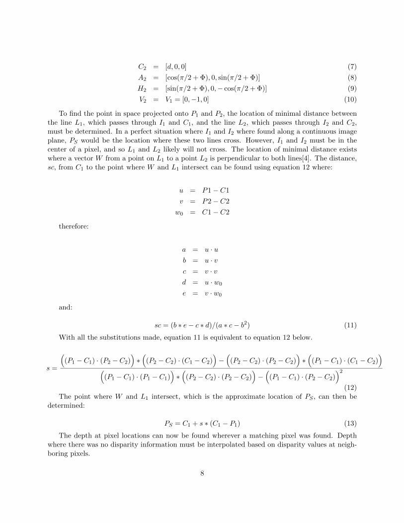
C2 = [d, 0, 0] (7)

A2 = [cos(π/2 + Φ), 0, sin(π/2 + Φ)] (8)

H2 = [sin(π/2 + Φ), 0,− cos(π/2 + Φ)] (9)

V2 = V1 = [0,−1, 0] (10)

To find the point in space projected onto P1 and P2, the location of minimal distance betweenthe line L1, which passes through I1 and C1, and the line L2, which passes through I2 and C2,must be determined. In a perfect situation where I1 and I2 where found along a continuous imageplane, PS would be the location where these two lines cross. However, I1 and I2 must be in thecenter of a pixel, and so L1 and L2 likely will not cross. The location of minimal distance existswhere a vector W from a point on L1 to a point L2 is perpendicular to both lines[4]. The distance,sc, from C1 to the point where W and L1 intersect can be found using equation 12 where:

u = P1− C1

v = P2− C2

w0 = C1− C2

therefore:

a = u · ub = u · vc = v · vd = u · w0

e = v · w0

and:

sc = (b ∗ e− c ∗ d)/(a ∗ c− b2) (11)

With all the substitutions made, equation 11 is equivalent to equation 12 below.

s =

((P1 − C1) · (P2 − C2)

)∗(

(P2 − C2) · (C1 − C2))−(

(P2 − C2) · (P2 − C2))∗(

(P1 − C1) · (C1 − C2))

((P1 − C1) · (P1 − C1)

)∗(

(P2 − C2) · (P2 − C2))−(

(P1 − C1) · (P2 − C2))2

(12)The point where W and L1 intersect, which is the approximate location of PS , can then be

determined:

PS = C1 + s ∗ (C1 − P1) (13)

The depth at pixel locations can now be found wherever a matching pixel was found. Depthwhere there was no disparity information must be interpolated based on disparity values at neigh-boring pixels.

8

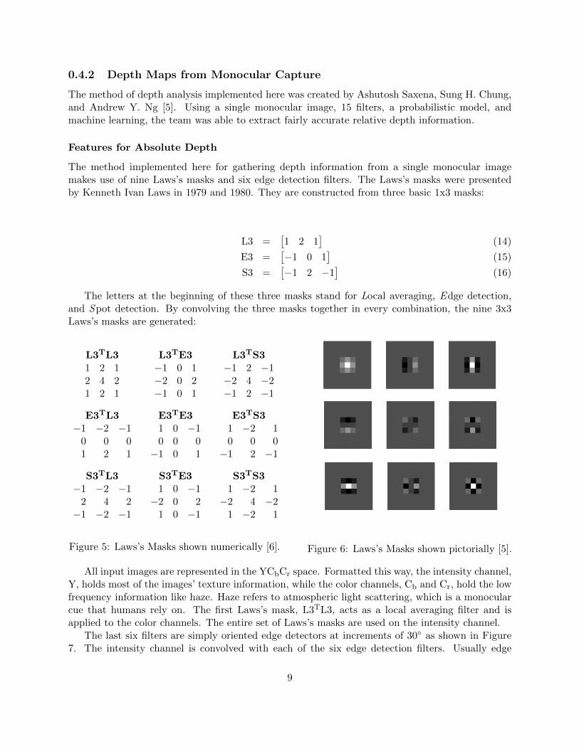
0.4.2 Depth Maps from Monocular Capture

The method of depth analysis implemented here was created by Ashutosh Saxena, Sung H. Chung,and Andrew Y. Ng [5]. Using a single monocular image, 15 filters, a probabilistic model, andmachine learning, the team was able to extract fairly accurate relative depth information.

Features for Absolute Depth

The method implemented here for gathering depth information from a single monocular imagemakes use of nine Laws’s masks and six edge detection filters. The Laws’s masks were presentedby Kenneth Ivan Laws in 1979 and 1980. They are constructed from three basic 1x3 masks:

L3 =[1 2 1

](14)

E3 =[−1 0 1

](15)

S3 =[−1 2 −1

](16)

The letters at the beginning of these three masks stand for Local averaging, Edge detection,and Spot detection. By convolving the three masks together in every combination, the nine 3x3Laws’s masks are generated:

L3TL31 2 12 4 21 2 1

L3TE3−1 0 1−2 0 2−1 0 1

L3TS3−1 2 −1−2 4 −2−1 2 −1

E3TL3−1 −2 −1

0 0 01 2 1

E3TE31 0 −10 0 0−1 0 1

E3TS31 −2 10 0 0−1 2 −1

S3TL3−1 −2 −1

2 4 2−1 −2 −1

S3TE31 0 −1−2 0 2

1 0 −1

S3TS31 −2 1−2 4 −2

1 −2 1

Figure 5: Laws’s Masks shown numerically [6]. Figure 6: Laws’s Masks shown pictorially [5].

All input images are represented in the YCbCr space. Formatted this way, the intensity channel,Y, holds most of the images’ texture information, while the color channels, Cb and Cr, hold the lowfrequency information like haze. Haze refers to atmospheric light scattering, which is a monocularcue that humans rely on. The first Laws’s mask, L3TL3, acts as a local averaging filter and isapplied to the color channels. The entire set of Laws’s masks are used on the intensity channel.

The last six filters are simply oriented edge detectors at increments of 30◦ as shown in Figure7. The intensity channel is convolved with each of the six edge detection filters. Usually edge

9

detection is done with a set of four or eight filters operating at 45◦ as in Sobel and Prewitt. Havingsix filters at 30◦, however, reduces the redundancy of eight filters, while still improving on just four.

Figure 7: Six edge detecting kernels oriented at 30◦ [5].

The product of the intensity channel convolved with the nine Laws’s masks, the two chromachannels convolved with the first Laws’s mask (local averaging filter), and the intensity channelconvolved with the six edge detecting kernels creates 17 output dimensions (Fn). Using equation17, where k = {1, 2}, the sum absolute energy and sum squared energy respectively can be foundby convolving the 17 output dimensions (Fn) with the original image, (I) . This creates the first34 dimensions of the feature vector for each pixel.

Ei(n) = Σ(x,y)∈patch(i)|I(x, y) ∗ Fn(x, y)|k (17)

To capture larger, more global features, three scales, or image resolutions are created. The firstscale exists at the pixel level and is represented in Figure 8 by the blue squares. The second scale,represented in Figure 8 in red, is produced by averaging the center blue pixel and its four adjacentblue pixels. Similarly, the third scale, represented in purple, is produced by averaging the center redpatch from scale two and its four red adjacent patches. Just as equation 17 was used on each patchin the original image(I) to create the first 34 dimensions of each patch’s feature vector, equation17 is also used on each neighboring patch, at each scale. The surrounding patches’ features aremade a part of the center patch’s feature vector, creating a total of 510 dimensions of informationat each pixel.

10

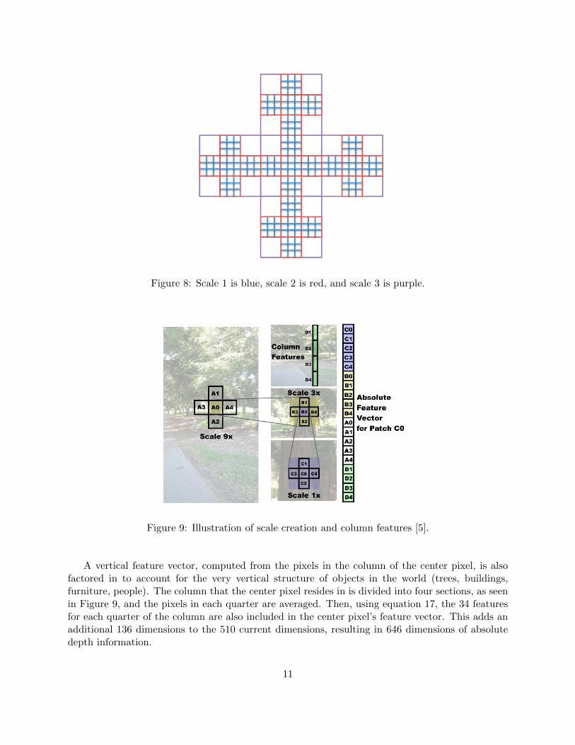
Figure 8: Scale 1 is blue, scale 2 is red, and scale 3 is purple.

Figure 9: Illustration of scale creation and column features [5].

A vertical feature vector, computed from the pixels in the column of the center pixel, is alsofactored in to account for the very vertical structure of objects in the world (trees, buildings,furniture, people). The column that the center pixel resides in is divided into four sections, as seenin Figure 9, and the pixels in each quarter are averaged. Then, using equation 17, the 34 featuresfor each quarter of the column are also included in the center pixel’s feature vector. This adds anadditional 136 dimensions to the 510 current dimensions, resulting in 646 dimensions of absolutedepth information.

11

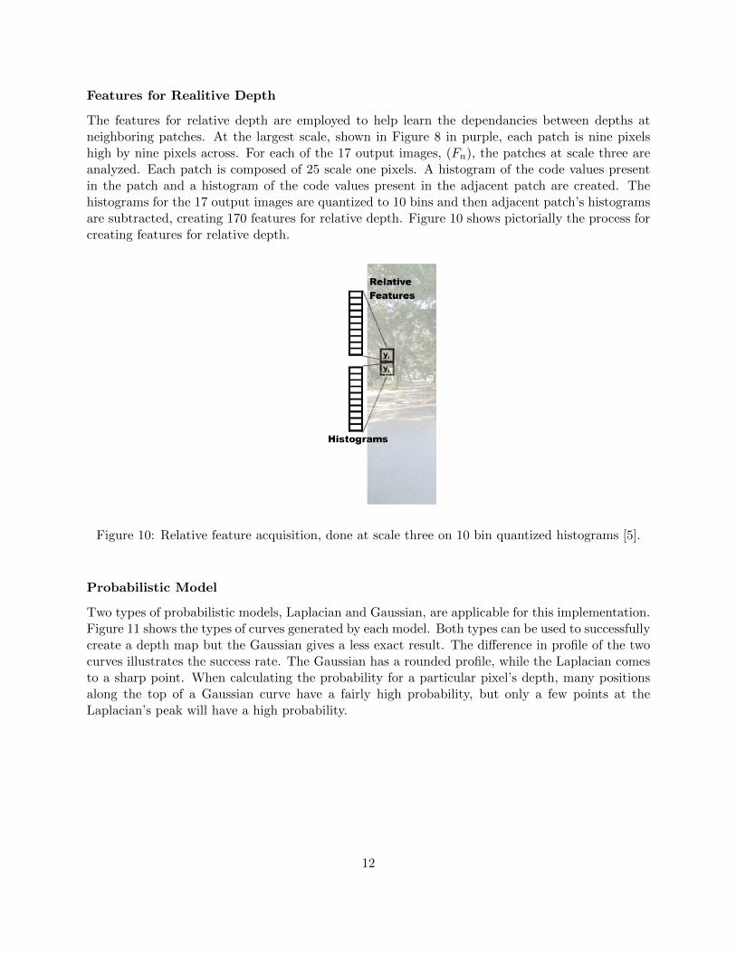
Features for Realitive Depth

The features for relative depth are employed to help learn the dependancies between depths atneighboring patches. At the largest scale, shown in Figure 8 in purple, each patch is nine pixelshigh by nine pixels across. For each of the 17 output images, (Fn), the patches at scale three areanalyzed. Each patch is composed of 25 scale one pixels. A histogram of the code values presentin the patch and a histogram of the code values present in the adjacent patch are created. Thehistograms for the 17 output images are quantized to 10 bins and then adjacent patch’s histogramsare subtracted, creating 170 features for relative depth. Figure 10 shows pictorially the process forcreating features for relative depth.

Figure 10: Relative feature acquisition, done at scale three on 10 bin quantized histograms [5].

Probabilistic Model

Two types of probabilistic models, Laplacian and Gaussian, are applicable for this implementation.Figure 11 shows the types of curves generated by each model. Both types can be used to successfullycreate a depth map but the Gaussian gives a less exact result. The difference in profile of the twocurves illustrates the success rate. The Gaussian has a rounded profile, while the Laplacian comesto a sharp point. When calculating the probability for a particular pixel’s depth, many positionsalong the top of a Gaussian curve have a fairly high probability, but only a few points at theLaplacian’s peak will have a high probability.

12

(a) Laplacian Probability Density Function (b) Gaussian Probability Density Function

Figure 11: Comparison of probability density curves after various manipulations.

The equation for a Gaussian curve is shown in equation 18.

f(x|µ, σ2) =1

σ√

2πexp

(−(x− µ)2

2σ2

)(18)

The equation for a Laplacian curve is shown in equation 19

f(x|µ, b) =1

2bexp

(−|x− µ|

b

)(19)

The Laplacian equation for modeling depth is shown in equation 20. It has the same basic formas equation 19 but computes one large summation from the product of many Laplacian curves.Equation 20 that was chosen for the depth estimation purposes here.

P (d|X; θ, λ) =1

Zexp

− M∑i=1

|di(1)− xTi θr|λ1r

−3∑

s=1

M∑i=1

∑j∈Ns(i)

|di(s)− dj(s)|λ2rs

(20)

Figure 12 shows the published results of the monocular depth map algorithm. The differencebetween Gaussian and Laplacian estimations are clearly visible in column three and four. The crisppoint of the Laplacian curve results in sharper edges as well as more accurate, uniform objects.The Gaussian gives a fair approximation of the scene but is outshone by the Laplacian results.

13

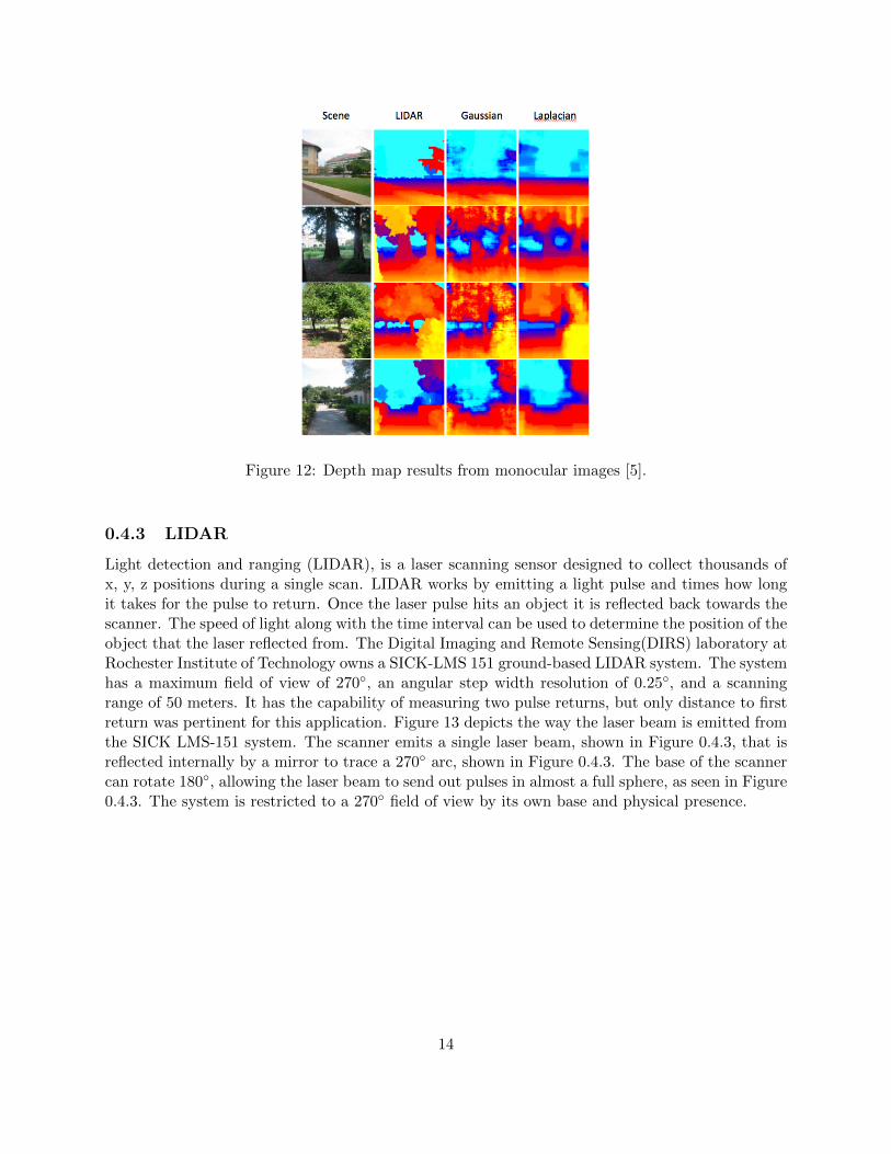
Figure 12: Depth map results from monocular images [5].

0.4.3 LIDAR

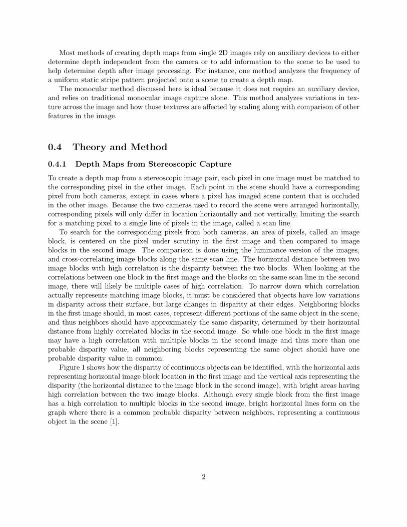
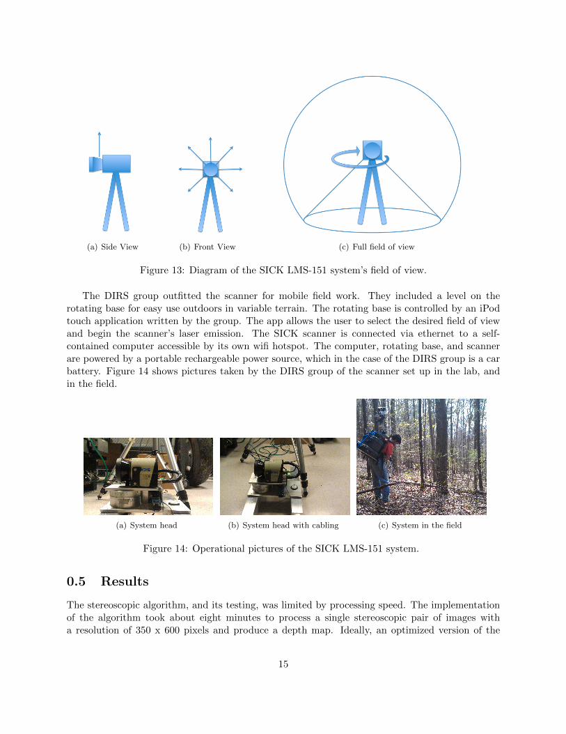
Light detection and ranging (LIDAR), is a laser scanning sensor designed to collect thousands ofx, y, z positions during a single scan. LIDAR works by emitting a light pulse and times how longit takes for the pulse to return. Once the laser pulse hits an object it is reflected back towards thescanner. The speed of light along with the time interval can be used to determine the position of theobject that the laser reflected from. The Digital Imaging and Remote Sensing(DIRS) laboratory atRochester Institute of Technology owns a SICK-LMS 151 ground-based LIDAR system. The systemhas a maximum field of view of 270◦, an angular step width resolution of 0.25◦, and a scanningrange of 50 meters. It has the capability of measuring two pulse returns, but only distance to firstreturn was pertinent for this application. Figure 13 depicts the way the laser beam is emitted fromthe SICK LMS-151 system. The scanner emits a single laser beam, shown in Figure 0.4.3, that isreflected internally by a mirror to trace a 270◦ arc, shown in Figure 0.4.3. The base of the scannercan rotate 180◦, allowing the laser beam to send out pulses in almost a full sphere, as seen in Figure0.4.3. The system is restricted to a 270◦ field of view by its own base and physical presence.

14

(a) Side View (b) Front View (c) Full field of view

Figure 13: Diagram of the SICK LMS-151 system’s field of view.

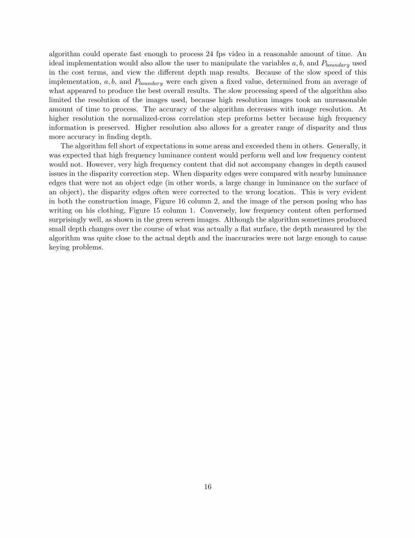
The DIRS group outfitted the scanner for mobile field work. They included a level on therotating base for easy use outdoors in variable terrain. The rotating base is controlled by an iPodtouch application written by the group. The app allows the user to select the desired field of viewand begin the scanner’s laser emission. The SICK scanner is connected via ethernet to a self-contained computer accessible by its own wifi hotspot. The computer, rotating base, and scannerare powered by a portable rechargeable power source, which in the case of the DIRS group is a carbattery. Figure 14 shows pictures taken by the DIRS group of the scanner set up in the lab, andin the field.

(a) System head (b) System head with cabling (c) System in the field

Figure 14: Operational pictures of the SICK LMS-151 system.

0.5 Results

The stereoscopic algorithm, and its testing, was limited by processing speed. The implementationof the algorithm took about eight minutes to process a single stereoscopic pair of images witha resolution of 350 x 600 pixels and produce a depth map. Ideally, an optimized version of the

15

algorithm could operate fast enough to process 24 fps video in a reasonable amount of time. Anideal implementation would also allow the user to manipulate the variables a, b, and Pboundary usedin the cost terms, and view the different depth map results. Because of the slow speed of thisimplementation, a, b, and Pboundary were each given a fixed value, determined from an average ofwhat appeared to produce the best overall results. The slow processing speed of the algorithm alsolimited the resolution of the images used, because high resolution images took an unreasonableamount of time to process. The accuracy of the algorithm decreases with image resolution. Athigher resolution the normalized-cross correlation step preforms better because high frequencyinformation is preserved. Higher resolution also allows for a greater range of disparity and thusmore accuracy in finding depth.

The algorithm fell short of expectations in some areas and exceeded them in others. Generally, itwas expected that high frequency luminance content would perform well and low frequency contentwould not. However, very high frequency content that did not accompany changes in depth causedissues in the disparity correction step. When disparity edges were compared with nearby luminanceedges that were not an object edge (in other words, a large change in luminance on the surface ofan object), the disparity edges often were corrected to the wrong location. This is very evidentin both the construction image, Figure 16 column 2, and the image of the person posing who haswriting on his clothing, Figure 15 column 1. Conversely, low frequency content often performedsurprisingly well, as shown in the green screen images. Although the algorithm sometimes producedsmall depth changes over the course of what was actually a flat surface, the depth measured by thealgorithm was quite close to the actual depth and the inaccuracies were not large enough to causekeying problems.

16

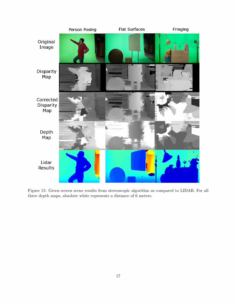
Figure 15: Green screen scene results from stereoscopic algorithm as compared to LIDAR. For allthree depth maps, absolute white represents a distance of 6 meters.

17

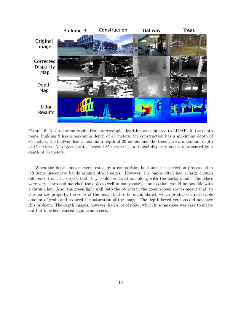
Figure 16: Natural scene results from stereoscopic algorithm as compared to LIDAR. In the depthmaps, building 9 has a maximum depth of 45 meters, the construction has a maximum depth of85 meters, the hallway has a maximum depth of 20 meters and the trees have a maximum depthof 85 meters. An object located beyond 85 meters has a 0 pixel disparity and is represented by adepth of 85 meters.

When the depth images were tested by a compositor, he found the correction process oftenleft some inaccurate bands around object edges. However, the bands often had a large enoughdifference from the object that they could be keyed out along with the background. The edgeswere very sharp and matched the objects well in many cases, more so than would be possible witha chroma key. Also, the green light spill onto the objects in the green screen scenes meant that, tochroma key properly, the color of the image had to be manipulated, which produced a noticeableamount of grain and reduced the saturation of the image. The depth keyed versions did not havethis problem. The depth images, however, had a lot of noise, which in some cases was easy to matteout but in others caused significant issues.

18

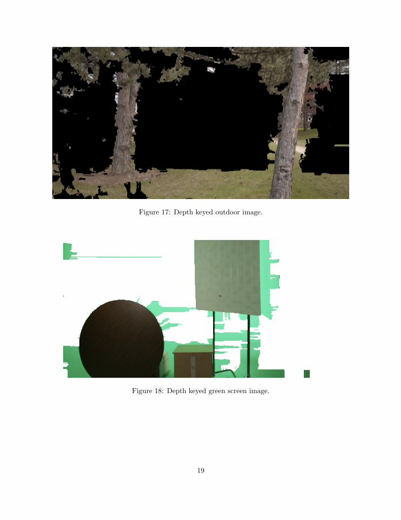
Figure 17: Depth keyed outdoor image.

Figure 18: Depth keyed green screen image.

19

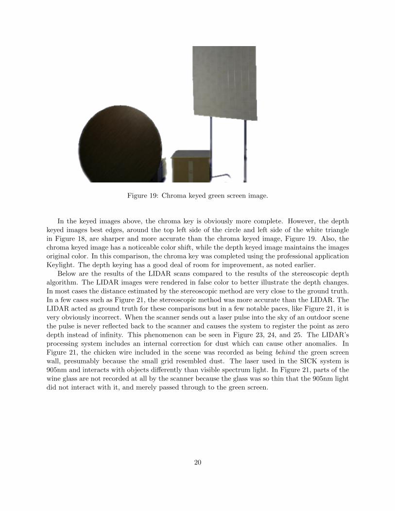
Figure 19: Chroma keyed green screen image.

In the keyed images above, the chroma key is obviously more complete. However, the depthkeyed images best edges, around the top left side of the circle and left side of the white trianglein Figure 18, are sharper and more accurate than the chroma keyed image, Figure 19. Also, thechroma keyed image has a noticeable color shift, while the depth keyed image maintains the imagesoriginal color. In this comparison, the chroma key was completed using the professional applicationKeylight. The depth keying has a good deal of room for improvement, as noted earlier.

Below are the results of the LIDAR scans compared to the results of the stereoscopic depthalgorithm. The LIDAR images were rendered in false color to better illustrate the depth changes.In most cases the distance estimated by the stereoscopic method are very close to the ground truth.In a few cases such as Figure 21, the stereoscopic method was more accurate than the LIDAR. TheLIDAR acted as ground truth for these comparisons but in a few notable paces, like Figure 21, it isvery obviously incorrect. When the scanner sends out a laser pulse into the sky of an outdoor scenethe pulse is never reflected back to the scanner and causes the system to register the point as zerodepth instead of infinity. This phenomenon can be seen in Figure 23, 24, and 25. The LIDAR’sprocessing system includes an internal correction for dust which can cause other anomalies. InFigure 21, the chicken wire included in the scene was recorded as being behind the green screenwall, presumably because the small grid resembled dust. The laser used in the SICK system is905nm and interacts with objects differently than visible spectrum light. In Figure 21, parts of thewine glass are not recorded at all by the scanner because the glass was so thin that the 905nm lightdid not interact with it, and merely passed through to the green screen.

20

Table 1: Green Screen: Table, nightstand, wall.

Point LIDAR Dist[m] 3D Dist[m] Discription

1 2.786 2.802 Nearest Wall2 3.102 3.113 Middle Wall3 3.541 3.502 Far Wall4 7.688 6.466 Green Screen

Figure 20: LIDAR results of table scene.

Table 2: Green Screen: Fringing objects.

Point LIDAR Dist[m] 3D Dist[m] Discription

1 6.27 3.113 Chicken Wire2 5.853 5.254 Green Screen3 0 2.335 Wine Glass4 1.597 2.335 Broom Bristles

Figure 21: LIDAR results of fringingscene.

21

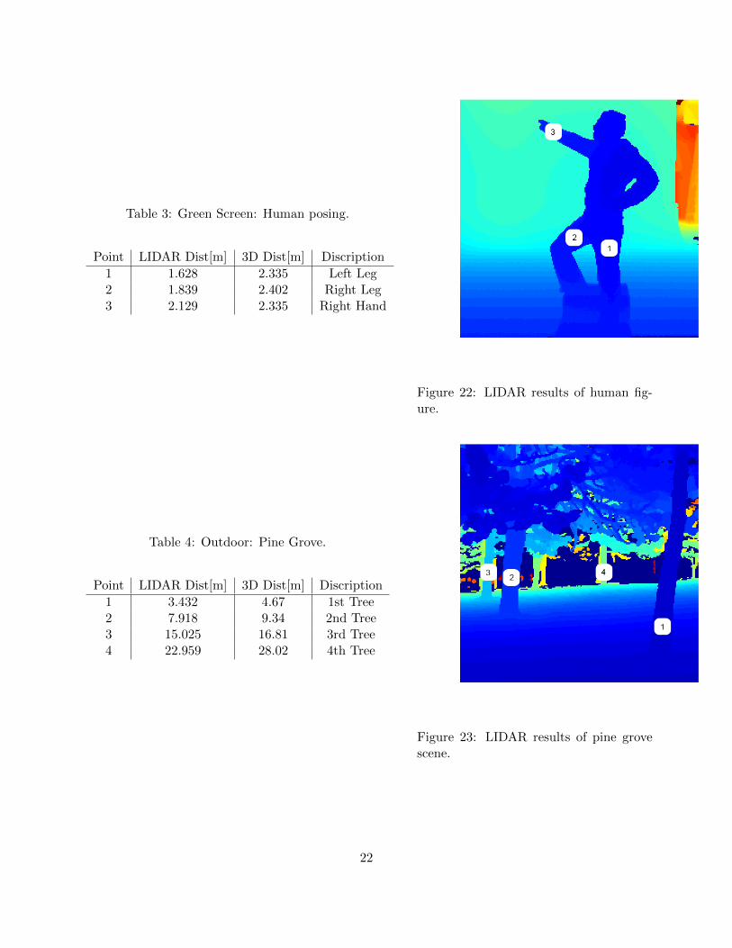
Table 3: Green Screen: Human posing.

Point LIDAR Dist[m] 3D Dist[m] Discription

1 1.628 2.335 Left Leg2 1.839 2.402 Right Leg3 2.129 2.335 Right Hand

Figure 22: LIDAR results of human fig-ure.

Table 4: Outdoor: Pine Grove.

Point LIDAR Dist[m] 3D Dist[m] Discription

1 3.432 4.67 1st Tree2 7.918 9.34 2nd Tree3 15.025 16.81 3rd Tree4 22.959 28.02 4th Tree

Figure 23: LIDAR results of pine grovescene.

22

Table 5: Outdoor: Building 9.

Point LIDAR Dist[m] 3D Dist[m]

1 18.708 21.022 24.64 28.023 28.088 28.024 38.758 42.03

Figure 24: LIDAR results of building ex-terior.

Table 6: Outdoor: Sculpture and construction behindbuilding 76.

Point LIDAR Dist[m] 3D Dist[m] Discription

1 14.059 14.01 Sculpture2 10.042 10.51 Base3 18.475 28.02 Further Base4 0

Figure 25: LIDAR results of constructionand sculpture scene.

23

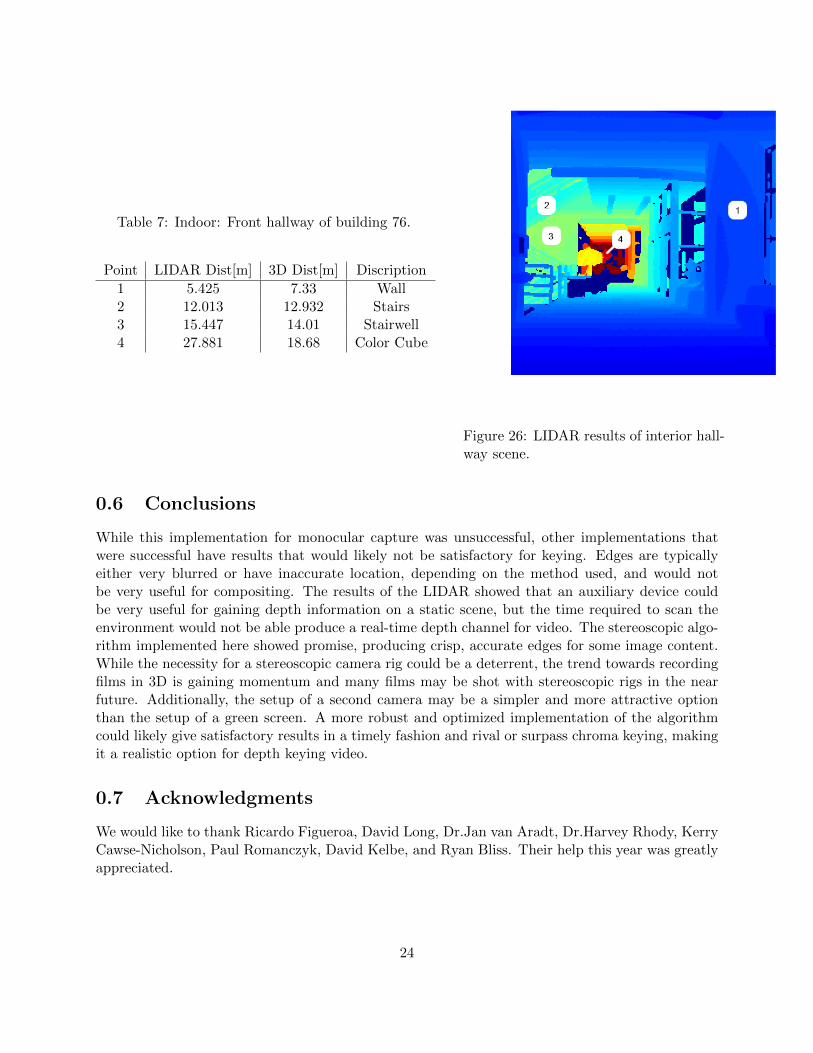
Table 7: Indoor: Front hallway of building 76.

Point LIDAR Dist[m] 3D Dist[m] Discription

1 5.425 7.33 Wall2 12.013 12.932 Stairs3 15.447 14.01 Stairwell4 27.881 18.68 Color Cube

Figure 26: LIDAR results of interior hall-way scene.

0.6 Conclusions

While this implementation for monocular capture was unsuccessful, other implementations thatwere successful have results that would likely not be satisfactory for keying. Edges are typicallyeither very blurred or have inaccurate location, depending on the method used, and would notbe very useful for compositing. The results of the LIDAR showed that an auxiliary device couldbe very useful for gaining depth information on a static scene, but the time required to scan theenvironment would not be able produce a real-time depth channel for video. The stereoscopic algo-rithm implemented here showed promise, producing crisp, accurate edges for some image content.While the necessity for a stereoscopic camera rig could be a deterrent, the trend towards recordingfilms in 3D is gaining momentum and many films may be shot with stereoscopic rigs in the nearfuture. Additionally, the setup of a second camera may be a simpler and more attractive optionthan the setup of a green screen. A more robust and optimized implementation of the algorithmcould likely give satisfactory results in a timely fashion and rival or surpass chroma keying, makingit a realistic option for depth keying video.

0.7 Acknowledgments

We would like to thank Ricardo Figueroa, David Long, Dr.Jan van Aradt, Dr.Harvey Rhody, KerryCawse-Nicholson, Paul Romanczyk, David Kelbe, and Ryan Bliss. Their help this year was greatlyappreciated.

24

Bibliography

[1] L. Falkenhagen, “Depth estimation from stereoscopic image pairs assuming piecewise continu-ous surfaces,” Tech. Rep., Institut fur Theoretische Nachrichtentechnik und Informationsverar-beitung Universitat Hannover, Hannover, Germany, n.d.

[2] I. J. Cox et al., “Stereo without disparity gradient smoothing: a bayesian sensor fusion solution,”in British Machine Vision Conference, 1992, pp. 337–346.

[3] Y. Yakimovsky, United States. National Aeronautics, Space Administration, and Jet Propul-sion Laboratory (U.S.), A System for Extracting 3-dimensional Measurements from a StereoPair of TV Cameras, NASA technical memorandum. Jet Propulsion Laboratory, CaliforniaInstitute of Technology, 1976.

[4] D. Sunday. (2006), Distance between Lines and Segments with their Closest Point of Approach,[Online]. Available: http://www.softsurfer.com.

[5] A. Saxena et al., “Learning depth from single monocular images,” Tech. Rep., ComputerScience Department, Stanford University, Stanford, CA.

[6] E.R. Davies, Machine Vision: Theory, Algorithms, Practicalities, 3rd ed., Oxford, UK: Elsevier,2005.

[7] P. Fua, “A parallel stereo algorithm that produces dense depth maps and preserves imagefeatures,” Machine Vision and Applications, vol. 6, no. 1, pp. 35–49, 1993.

25