School of Economics and Management Aarhus University

Bartholins Allé 10, Building 1322, DK-8000 Aarhus C Denmark

CREATES Research Paper 2010-53

Detecting Housing Submarkets using Unsupervised Learning of Finite Mixture Models

Christos Ntantamis

Detecting Housing Submarkets using Unsupervised Learning of

Finite Mixture Models

Christos G. Ntantamis ∗

Aarhus University, CREATES

August 18, 2010

Abstract

The problem of modeling housing prices has attracted considerable attention due to its importance

in terms of households’ wealth and in terms of public revenues through taxation. One of the main

concerns raised in both the theoretical and the empirical literature is the existence of spatial association

between prices that can be attributed, among others, to unobserved neighborhood effects. In this paper,

a model of spatial association for housing markets is introduced. Spatial association is treated in the

context of spatial heterogeneity, which is explicitly modeled in both a global and a local framework. The

global form of heterogeneity is incorporated in a Hedonic Price Index model that encompasses a nonlinear

function of the geographical coordinates of each dwelling. The local form of heterogeneity is subsequently

modeled as a Finite Mixture Model for the residuals of the Hedonic Index. The identified mixtures are

considered as the different spatial housing submarkets. The main advantage of the approach is that

submarkets are recovered by the housing prices data compared to submarkets imposed by administrative

or geographical criteria. The Finite Mixture Model is estimated using the Figueiredo and Jain (2002)

approach due to its ability in endogenously identifying the number of the submarkets and its efficiency

in computational terms that permits the consideration of large datasets. The different submarkets are

subsequently identified using the Maximum Posterior Mode algorithm. The overall ability of the model

to identify spatial heterogeneity is validated through a set of simulations. The model was applied to

Los Angeles county housing prices data for the year 2002. The results suggests that the statistically

identified number of submarkets, after taking into account the dwellings’ structural characteristics, are

considerably fewer that the ones imposed either by geographical or administrative boundaries.

JEL Classification Numbers: C13, C21, R0Keywords: Hedonic Models, Finite Mixture Model, Spatial Heterogeneity, Housing Submarkets

∗Address: School of Economics & Management, University of Aarhus, Building 1322, 8000 Aarhus C, Denmark, telephone:+45 89422140, email: cntantamis@creates.au.dk. This paper constitutes the first part of my PhD thesis in McGill University. Iwould like to express gratitude to Professor Leah Brooks for providing me with the data and for her suggestions, and to ProfessorJohn W. Galbraith for helpful comments. I also benefited from invaluable comments from the participants of the Society forComputational Economics International Conference in Montreal, of the Canadian Economics Association Annual Meeting,inHalifax, and the Department of Economics Ph.D. Seminars, McGill University. Any remaining errors are my own. Center forResearch in Econometric Analysis of Time Series, CREATES, is funded by The Danish National Research Foundation.

1

1 Introduction

The problem of modeling dwelling selling prices is still a challenge for housing analysts, especially in view ofthe importance that real estate wealth has in the household’s consumption and thus in the entire economy.Hedonic market models, which are observed on the equilibrium between demand and supply at a given time,have been used for this purpose as a common modeling approach. Hedonic models (or indexes) considerthe features of an asset to be the determinants of its actual values. Consequently, a house price can beestimated by regressing on the number of rooms, the total living area, the number of bathrooms, andlocation characteristics. However, it is very difficult to get a complete account of all the relevant locationcharacteristics, so the regression residuals are often found to be spatially correlated.

The latter issue emerges as a direct consequence of the nature of housing compared to other commodities.In particular, housing differs in terms of its high cost, its durability, its heterogeneity, and most importantlyits locational fixity. The intrinsic uniqueness of each location gives rise to the spatial heterogeneity propertyof housing.

Geographic data are predominantly dependent. As Tobler (1970) suggests in his First Law of Geography

“Everything is related to everything else, but near things are more related than distant things”

This spatial heterogeneity needs to be modeled in order not only to improve the efficiency of the hedonicmodels estimates, but also to incorporate this spatial information in order to construct more effective modelsfor housing valuations. In the literature there are two approaches to modeling spatial heterogeneity. Thefirst one attempts to model directly the autocorrelation structure of the hedonic model residuals. Dubin(1992,1998) makes use of kriging in order to model the residuals; their correlation is written as a functionof the distance between two dwellings 1. In a similar fashion, Basu and Thibodeau (1998) model the spatialautocorrelation of the residuals using semi-variograms. On the other hand, Can (1992), Can and Megbolugbe(1997), and Dubin et al. (1999), building on Anselin’s (1988) model of spatial autocorrelation, incorporatespatially lagged variables directly in the hedonic regression. The estimation of these models requires theconstruction of weight matrices, which are square matrices with dimension equal to the number of theobservations so as to state the spatial autocorrelations, and their subsequent inversion. When the numberof observations becomes large, inverting the weight matrix becomes problematic even though this effect ismitigated by the fact that the matrix is sparse.

The second approach to modeling spatial heterogeneity builds on the presumption that we can segmenthousing markets to clusters of dwellings that need to satisfy the following three conditions2: (a) homogeneity,(b) contiguity, and (c) parsimony. Each cluster should constitute a different housing submarket. Thus, thehedonic model, when estimated for dwellings within each cluster, may be able to provide residuals that arespatially uncorrelated. This presumption has its origins in the early housing markets literature. Strazsheim(1974) states:

“The urban housing market” is a set of compartmentalized and unique submarkets withdemand and supply influences likely to result in a different stucture of prices in each.”

1Kriging corresponds to a set of geostatistical techniques to interpolate the value of a random field at an unobserved locationfrom observations of its value at nearby locations.

2Goodman (1981).

2

Housing markets may be away from the long-run equilibrium as a result of segmented demand or in-flexible supply adjustment processes. The standard long-run analysis assumes instantaneous adjustment ofhousing size, location, quality and distribution of dwelling units to changes in income, employment, location,population, tastes, and transportation (see Strazheim 1975). On the demand side, however, it has beennoticed that prospective owners and renters often examine housing in a limited geographical area because ofsearch costs, racial discrimination, or desired proximity to friends or workplace. On the supply side, thereare also constraints; capital stock is difficult to modify, and vacant land is scarce especially in urban regions.

The first part of the paper follows the approach of Goodman (1981) and thus it models the spatialheterogeneity in housing prices in the submarkets setting. This approach emphasizes classification accountingfor spatial heterogeneity, by making groups of observations define potential submarkets. In contrast to alarge part of the literature that defines the location of the submarkets a priori, based on socioeconomicconsiderations, political jurisdictions, school districts or market areas as perceived by the real estate agencies(for example Goodman 1981, Adair et al. 1996, and Goodman and Thibodeau 1998), I estimate the numberand the location of the submarkets endogenously. That is, instead of determining the submarkets based onsome prior view, an alternative approach that allows the data to speak for themselves is followed. Examplesfrom the literature following the same approach include, among others, Clapp et al. (2002), Ugarte et al.(2004) and Clapp and Wang (2005).

This method allows the researchers to model rather than impose submarkets. The number and thecorresponding locations of the submarkets will be determined in an optimal way, i.e. in terms of the data’sstatistical properties, in order to identify the areas with similar demand and supply functions. Thus, itis expected that the model will identify housing submarkets in a more parsimonious way compared withthe determination of submarkets solely in terms of geographically determined or administratively imposedregions. What may appear to be diverse submarkets could in fact be artificial divisions.

In this paper, I propose a model that consists two modules. The first module involves an extendedversion of the hedonic price model; the geographical coordinates of the dwelling are included to the set ofthe explanatory variables, as in Clapp and Wang (2005). The hedonic model is estimated using a standardOLS procedure. This yields prices that are standardized for the dwelling’s structural characteristics. Thesecond module assumes that the residuals from the first module follow a Finite Mixture Model, with eachof the mixing components corresponding to a housing submarket. I consider this approach as intuitivelyappealing; there is a one-to-one correspondence between the mixtures and the housing submarkets.

Similar problems are addressed in engineering applications such as image processing or pattern recognitionand as a result a rather voluminous literature has been formed over the past years. The methods that areproposed in this literature present desirable properties both in terms of estimation accuracy and computationefficiency.

I use the Minimum Description Length criterion variant proposed by Figuereido and Jain (2002) for theestimation of the Finite Mixture Model. The particular approach is selected for these merits: a) the numberof the mixtures, and thus the number of the housing submarkets, are endogenously identified during theestimation, b) the model estimation algorithm is simple in its implementation since it includes a variant ofthe standard Expectation Maximization algorithm, and c) it is computationally more efficient, thus allowingthe examination of considerably larger data sets (100000 dwellings or more), which makes the methodology

3

appropriate for mass assessment applications 3.The final step of the modeling procedure is the re-estimation of the hedonic model for each of the identified

spatial submarkets. The parameters of the index can be subsequently used in order to obtain the value forany dwelling that belongs to that submarket.

Nowhere in the previous literature were Monte Carlo simulations used to validate the ability of the modelsto identify spatial clusters. Here, this evaluation of the validity of the model is undertaken with the resultindicating that the model can be used for the identification of housing submarkets and for the explanationof the price variation, in data sets containing a large number of observations.

Finally, the model is employed in order to scrutinize the housing market of the Los Angeles county usingvalues of houses sold in year 2002. The sample size obtained is considerably larger compared to what is usedin past empirical applications (approximately 108000 dwellings). The results suggest that the statisticallyidentified number of submarkets, after taking into account the dwellings’ structural characteristics, areconsiderably fewer by far than the ones imposed either by geographical or administrative boundaries.

The remaining chapter is structured as follows: Section 2 describes the model used in the analysis indetail. The hedonic price model is reviewed and the estimation procedure for the finite mixture model isintroduced. Section 3 discusses the simulation results. In section 4, the results from the application ofthe model to the real estate market of Los Angeles are presented. The chapter ends with some concludingremarks.

2 The model

2.1 The hedonic model

Since the seminal work of Adelman and Griliches (1961), who provided the rational for the construction ofhedonic indices as a quantification of heterogeneous products’ quality, a vast literature for the determinationof housing prices has emerged. Rosen (1974) provided the theoretical framework for the hedonic models asan approach to the determination of housing prices. He argued that in equilibrium between demand andsupply, the price of the house can be determined as a function of its characteristics and the weights can beestimated by running a standard regression. Moreover, Rosen (1974) and Epple (1987) discussed the issuesinvolved in how to obtain the demand and/or supply functions from the estimated hedonic model.

The hedonic price model can be written as

y = X · β + ε (1)

where y is the dependent variable related with the dwelling price and X corresponds to the set of the dwellingcharacteristics such as lot size, number of bedrooms, existence of fireplace, neighborhood amenities, etc. Themodel is estimated by Ordinary Least Squares.

Despite its age, the hedonic model approach is still very popular for housing market valuation. It ispreferred over the usual repeat-sales approach used by appraisers as it has been demonstrated (Meese andWallace 1997, Pace et al 2002) that: a) it actually yields smaller errors in terms of forecasting the realized

3Data sets in the existing literature involve a number of housing prices in the vicinity of 1000, for example Adair et al.(1996) consider 1080 transactions, Clapp and Wang (2005)’s sample was of 1069 transactions.

4

market price, and b) it enables a rather costless evaluation for every new property once the parameters ofthe hedonic model have been estimated.

There are several issues regarding the specification of the hedonic model, as discussed extensively inFreeman (1979), Mark and Goldberg (1988), Meese and Wallace (1997), Basu and Thibodeau (1998), Reichert(2002), and Pace et al. (2002) but the most important are related to the functional form and to variableselection priority.

Rosen (1974) did not preclude any particular form for the function of the characteristics; the hedonicfunction could very well take a nonlinear form. The literature addresses the problem of the functional formby considering a Box-Cox transformation of the data. The most usual functional formulations are the semi-log (the log of the price is the dependent variable, whereas the structural characteristics remain unaltered),or the log-log (all variables in the regression function are taken in logs). In this paper the semi-log formis employed for several reasons: a) it is used in the majority of the recent literature, b) it decreases theheteroskedasticity in the residuals, and c) it provides a neat interpretation of the estimated coefficients ofthe regressions (rate of change in the price for an additional unit of the structural variable).

The dwelling characteristic variables can be separated into two categories. The first one corresponds withthe structural characteristics of the dwelling such as age, lot size, number of rooms, existence of pool, etcthat can be measured with relative accuracy. The second one corresponds with the neighborhood character-istics such as racial composition, amenities, environmental aspects, etc, which generate the most problems.Modeling all the neighborhood effects in a coherent way is challenging due to difficulties in identifying thedifferent effects, and in constructing proper quantitative variables for their description. The problem ofomitted variables which will result in biased and inconsistent estimates for the model will inevitably emerge.Moreover, quantifying the quality aspects of the particular neighborhood is very cumbersome as it will requirethe construction of detailed questionnaires to be completed by a significant number of objective evaluators(Kain and Quigley 1970). Finally, such a task is simply implausible for the case of Mass Assessment whenthe task involves estimating the value of all dwellings in a large city.

In order to circumvent these issues, neighborhood characteristics will not be included in the analysis asit has been argued before that the explicit modelling of the spatial heterogeneity can capture these effects.

Lastly, a “global” form of heterogeneity is incorporated in the hedonic model by encompassing a non-linear function of the geographical coordinates of each dwelling. The acquisition of the coordinates is madepossible by the use of geocoding (a Geographic Information Systems (GIS)application that allows the exactpinpointing of each dwelling, based on its address, in terms of its geographical coordinates). The coordinatesfunction operates as a proxy for location-specific information. This method is preferred to the one thatsimply puts neighborhood dummy variables since it leaves less space for arbitrary decisions such as theselection of the neighborhoods’ boundaries 4. Moreover, since the focus of this paper is in the endogenouslyidentification of submarkets the employment of information of that type is not desirable.

2.2 Finite mixture Model

The hedonic price model takes into account the structural characteristics of the dwelling. The spatialattributes will be estimated by assuming a finite mixture model for the residuals from the OLS estimation

4The selection of the neighborhoods can be done on a variety of criteria (administrative-type boundaries like postal codesand census tracts, or geographical boundaries like rivers, roads, andrail-tracks) that do not provide a unique answer.

5

of the hedonic model. The number of mixtures identified will correspond with the number of the differentsubmarkets the housing market is segmented into. In what follows, the Finite Mixture Model is presentedalong with the standard approach used for its estimation (the Expectation Maximization EM algorithm).Subsequently, the Minimum Description Length criterion variant proposed by Figuereido and Jain (2002)will be presented and its relative merits over EM approaches will be discussed. In the folllowing sections,the random variables Y used in the exposition of the model will correspond to the residuals obtained fromthe hedonic model, each residual representing a different dwelling.

2.2.1 The Finite Mixture Model and the EM algorithm

Let Y = [Y1, . . . , Yd]T be a d -dimensional random variable, with y = [y1, . . . , yd]T representing one particularoutcome of Y. It is said that Y follows a k -component finite mixture distribution if its probability functioncan be written as:

p (y| θ) =k∑

m=1

αmp (y| θm) (2)

where α1, . . . , αk are the mixing probabilities, θm corresponds with the parameters defining the mth distri-butional component, and θ ≡ {θ1, . . . , θk, α1, . . . , αk} is the complete set of parameters needed to define themixture. The mixing probabilities αm satisfy the following conditions:

αm ≥ 0, m = 1, . . . , k, andk∑m

αm = 1 (3)

Given the set Y ={y(1), . . . ,y(n)

}of n independent and identically distributed samples, the log-likelihood

corresponding to a k -component mixture is

log p (Y| θ) = logn∏i=1

p(y(i)|θ) =n∑i=1

logk∑

m=1

αmp(y(i)|θm) (4)

The Maximum likelihood (ML) estimate can not be found analytically. The usual choice for estimating theparameters of the mixture model is the employment of the Expectation Maximization (EM) algorithm. EMis an iterative procedure that finds the local maxima of the log p (Y| θ) and is extensively discussed in thework of McLachlan and Peel (2000) for the case of finite mixtures.

The EM algorithm is based on the interpretation that the data are incomplete. In the case of finitemixtures, the missing part is a set of n labels Z =

{z(1), . . . , z(n)

}associated with the n samples, indicating

which component produced each sample. Each label is a binary vector z(i) = [z(i)1 , . . . , z

(i)k ], where z(i)

m = 1and z(i)

p = 0 for p 6= m, which means that the sample y(i) was produced by the mth component. Consequently,the complete log-likelihood can be written as

log p (Y,Z| θ) =n∑i=1

k∑m=1

z(i)m logαmp(y(i)|θm) (5)

The EM algorithm results in a sequence of estimates{θ(t), t = 0, 1, 2, . . .

}by iteratively applying 2 alternate

steps:

6

• E-step: Computes the conditional expectation of the complete log-likelihood, given Y and the currentestimate θ(t). Since log p (Y,Z| θ) is linear with respect to the missing data Z, we have to computethe conditional expectation W = E[Z | Y, θ(t)] and then plug it back into the complete log-likelihood.The result is the so-called Q-function:

Q(θ, θ(t)) ≡ E[log p (Y,Z| θ) | Y, θ(t)

]= log p (Y,W| θ) (6)

Since the elements of Z are binary, their conditional expectations are given by

w(i)m ≡ E

[z(i)m |Y, θ(t)

]= Pr

[z(i)m = 1|y(i), θ(t)

](7)

=αm(t) p(y(i)|θm(t))∑kj=1 αj(t) p(y(i)|θj(t))

(8)

• M-step: Updates the parameter estimates according to

θ(t+ 1) = arg maxθ

{Q(θ, θ(t)) + log p(θ)

}(9)

under the constraints of (3).

The problem with working with the EM algorithm is that it assumes that the number of mixture components kis known. This is never the case in real applications. The employment of the ML criterion is not appropriate;the class of the k-component models (Mk) is nested in the class of the (k+1) components model (Mk+1), andthus the likelihood will be increasing even if an extra, unnecessary mixture component is added. Alternativemethods have been proposed in order to estimate the number of the mixture distributions. The most commonones are of a deterministic nature. A set of candidate models is estimated using EM for a range of valuesof k (k ∈ [kmin, . . . , kmax]) which is assumed to contain the true value of k. The number of components canthen be determined according to

k = arg mink

{C(θ(k), k

), k = kmin, . . . , kmax

}(10)

where C(θ(k), k

)is some selection criterion and θ(k) is the estimate of the set of the mixture parameters

for the given k. The usual form of these criteria is:

C(θ(k), k

)= − log p (Y| θ(k)

)+ P(k) (11)

where P(k) is an increasing function penalizing higher values of k. Such criteria are Approximate Bayesiancriteria ( Laplace-empirical criterion LEC, Bayesian inference criterion BIC), approaches based on informa-tion/coding theory concepts (Akaike’s information criterion AIC, Minimum message length criterion MML),and methods based on the complete likelihood (5) (Classification likelihood criterion CLC, Integrated clas-sification likelihood criterion ICL). For a more detailed review and comparison of these methods, the readeris directed to McLachlan and Peel (2000).

7

2.2.2 The Figuereido and Jain (2002) Minimum Message Length Criterion variant

The deterministic methods discussed in the previous section select a model class Mk based on its “best”representative θ(k). Nevertheless, in the mixture models, the distinction between model-class selection andmodel estimation is unclear, e.g. a 3-component mixture with one mixing probability equal to zero cannot be distinguished from a 2-component mixture. Moreover, EM algorithms are known to suffer from twomajor drawbacks: (a) they are highly dependent on initialization values, and (b) they may converge tothe boundary of the parameter space. Potential methods to correct for (a), include among others repeatedapplications of the EM algorithm for different initialization schemes. Nevertheless, these approaches demanda lot of computation time.

Figuereido and Jain (2002) proposed a different approach in order to circumvent these issues. Theyproposed a Minimum Message Length (MML) criterion that endogeneizes the selection of the optimal k.This is achieved by attempting to identify the “best” overall model in the entire set of available models

kmax⋃kmin

Mk

rather than selecting one among a set of candidate models.The main idea behind minimum encoding length criteria (like MML and MDL) is that a model is a good

one if it can be described by using a short code for the data. Consider some dataset Y that it is knownto have been generated according to the probability model p (Y| θ). Our goal is to encode the data andtransmit them without any loss of information. If p (Y| θ) is known to both the transmitter and the receiver,then they can both build the same code and communicate. However, if the parameters θ are unknown, thetransmitter first needs to estimate them and subsequently transmit them. This leads to a two-part message,whose total length is given by

Length (θ,Y) = Length (θ) + Length (Y| θ) (12)

All minimum encoding length criteria state that the parameter estimate is the one that minimizesLength (θ,Y).Figuereido and Jain (2002) obtained the following form of the MML criterion (derived in their Appendix),where the minimization with respect to θ is simultaneous in both θ (the parameter space) and its dimensionc:

θ = arg minθ

{− log p (θ)− log p (Y| θ) +

12

log |I (θ)|+ c

2

(1 + log

112

)}(13)

where I (θ) ≡ −E[D2θ log p (Y| θ)

]is the (expected) Fisher information matrix and |I (θ)| denotes its deter-

minant5.The MDL criterion can be obtained as an approximation to (13) and is given by

cMDL = arg minc

{− log p (Y| θ (c)

)+c

2log n

}(14)

whose two-part code interpretation is clear: − log p (Y| θ (c))

is the data code-length, while each of thec parameter set components requires a code-length proportional to (1/2) log n. Nevertheless, I (θ) is not

5D2θ denotes the Hessian matrix.

8

available, in general, in analytical form for the case of mixtures. In order to circumvent this problem, wereplace it by the complete-data Fisher information matrix Ic (θ) ≡ −E

[D2θ log p (Y,Z| θ)

], which is an upper

bound for I (θ). The authors adopt a prior expressing lack of knowledge about the mixing parameters. Inmore detail

1. The parameters of the different components are assumed to be a priori independent and also indepen-dent of the mixing probabilities:

p (θ) = p (α1, . . . , αk)k∏

m=1

p (θm)

2. For each factor p (θm) and p (α1, . . . , αk), the standard noninformative Jeffrey’s prior is adopted

p (θm) ∝√∣∣I(1) (θm)

∣∣p (α1, . . . , αk) ∝

√|M| = (α1α2 . . . αk)−1/2

for 0 ≤ α1, α2, . . . , αk ≤ 1 and α1 + α2 + . . .+ αk = 1.

Given the above assumption and noticing that for a k -mixture the dimension of θm is c = Nk+ k, whereN is the number of the parameters for each of the mixture distributions, (13) becomes

θ = arg minθL (θ,Y) (15)

with

L (θ,Y) =N

2

k∑m=1

log(nαm

12

)+k

2log

n

12+k(k + 1)

2− log p (Y| θ) (16)

The following intuitive interpretation can be given to this criterion:

1. − log p (Y| θ) is the code-length of the data.

2. The expected number of points generated by the mth component is nαm; this can be thought of as theeffective sample size for the estimation of θm. This gives rise to the term (N/2) log(nαm).

3. The αm’s are estimated from all n observations, giving rise to the term (k/2) log(n).

The objective function in (16) does not make sense if any of the αm’s is equal to zero (it becomes −∞).Regardless, the only thing that we need to code and transmit are the mixing elements whose probability isnonzero. Defining by knz the number of the nonzero probability components, (16) becomes

L (θ,Y) =N

2

∑m:αm>0

log(nαm

12

)+knz2

logn

12+knz(k + 1)

2− log p (Y| θ) (17)

Figueiredo and Jain (2002) also provide the variant of the EM algorithm that is necessary to estimatethe finite mixture using (17). In particular, for fixed knz, the E-step is

9

αm(t+ 1) =max

{0,(∑n

i=1 w(i)m

)− N

2

}∑kj=1 max

{0,(∑n

i=1 w(i)j

)− N

2

} , (18)

m = 1, 2, . . . , k

whereas the M-step is

θ(t+ 1) = arg maxθQ(θ, θ(t)), for m : αm(t+ 1) > 0 (19)

In the case of univariate Gaussian mixture models, each of the mixing distributions is fully specified byits mean and variance, i.e. θm =

(µm, σ

2m

). The M-step of the EM algorithm is then summarized in the

following two equations:

µm(t+ 1) =

(n∑i=1

w(i)m

)−1 n∑i=1

y(i)w(i)m (20)

σ2m(t+ 1) =

(n∑i=1

w(i)m

)−1 n∑i=1

(y(i) − µm(t+ 1)

)2

w(i)m (21)

In order to improve the speed of convergence and to avoid problems that EM presents, such as sensitivityto initial conditions, the authors use the Component-Wise Expectation Maximization Algorithm (CEM2)proposed by Celeux et al. (1999). CEM2 permits the parameters’ estimation of one mixture distribution ateach iteration. Celeux et al. (1999) prove the convergence properties of CEM2 by using the fact that EMfalls into a class of iteration methods called Proximal Point Algorithms (Chretien and Hero III 2000).

2.2.3 Recovering the location of the submarkets

It was stated earlier that the number of submarkets will be equal to the estimated number of the mixingdistibutions. Given the estimates from the finite mixture model, it is necessary to provide a decision rule thatwill reconstruct the market segments. In order to do so, the Maximum Posterior Mode (MPM) algorithmwill be used. The MPM algorithm assigns to each data point, here each dwelling, the mixing distributionthat is the most probable to have generated the particular point value. More specifically, the data point (i)is allocated to the mth distribution if

w(i)m > w

(i)j ,

(j = 1, 2, . . . , k

)(22)

where w(i)m comes from (7). The different submarkets are then defined as the collection of the housing data

points assigned to each distribution.

3 Simulation Results

The proposed methodology for the identification of regions has been introduced in the context of engineeringapplications, such as image segmentation problems where the input data are pixel intensities. Thus, it is

10

of interest to examine the performance of the method when economic data, such as housing prices, areconsidered. Two different types of simulations were performed in order to examine the ability of the modelto identify housing submarkets. The first one involved the simple case of identifying regions defined by pointsgenerated as independent draws from different distributions. The second one attempted to imitate a genuineproblem by considering a hypothetical housing market divided into different submarkets.

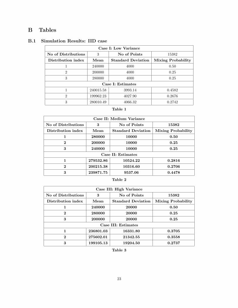
3.1 Case I: IID regions

This set of simulations investigated the performance of the estimation procedure for the finite mixture modelalone. An two-dimensional area was divided into three different segments. Each segment contained pointsgenerated independently by a Normal distribution. I considered three different cases of increasing variabilityfor the values of the points. The theoretical parameters for each distribution and their correspondingestimates are summarized in Tables 1 to 3.

The following criteria need to be satisfied for ensuring the validity of the proposed model. The firstcriterion concerns the correct estimation of the underlying distributions’ parameters; the estimates obtainedwere quite accurate being more precise for low-variability data. The second criterion corresponds to thecorrect identification of the segments’ boundaries; Figures 1 to 3 depict the identified segments as a collectionof points in space with different colors. Points with the same color were identified to have been generatedfrom the same distribution, i.e. belonging to the same submarket. The separation of the different coloredsegments is visible in the figures. Once more, the level of separation was more precise for the low andmedium-variability data. The last criterion amounts to the degree of homogeneity within each identifiedsegment; high level of homogeneity will be represented in the figures by high color homogeneity as well. Thedegree of homogeneity is excellent for the low-variability data (Figure 1), where the segments do not containpoints that are attributed to a different segment (100% homogeneous segments) ,very good for the medium-variability data (Figure 2), where the segments do contain a few points that are attributed to a differentsegment (approximately 99% homogeneous segments), and good for the high-variability data (Figure 3),where the segments are, on average, approximately 10% homogeneous. Thus, misclassification of points to adifferent that their true segment may occur at most at 10% of the time, which can be considered acceptable.

Overall, the performance of the model in terms of the aforementioned criteria was good, especially forthe cases of the low and the medium variance of the underlying distributions.These results validated themodel’s adequacy in estimating finite mixture model for at least the simple case of IID regions.

3.2 Case II: Submarkets

The case of IID regions is not very realistic. Hence the ability of the proposed model should be tested incases that emulate an actual housing market as much as possible. In order to do so, a hypothetical housingmarket segmented into seven different submarkets (see Figure 4) was constructed. For each submarket, ahedonic model based on a set of structural characteristics was assumed. The structural characteristics’ valueswere created using a variety of distributional configurations. The details of this procedure are presented insection 2.6.

Preliminary results obtained from the estimation on the Los Angeles data were used for calibrating thesimulation parameters. Most of the structural characteristics’ values were generated independently from

11

the values of other characteristics. The only exceptions were the values for the number of bathrooms (thecorrelation with the number of bedrooms was about 0.85), the values for the structure area (the correlationwith the number of bedrooms was about 0.87), and whether the dwelling would have a garage or not (thecorrelation with the existence of a fireplace was about 0.69). The following functional form that was assumedin order to generate the dwelling log prices for each of the assumed seven submarkets is6:

log(SV ) = α+ β1lot+ β2structure+ β3age+ β4bed+ β5bath/bed

+ β6fireplace+ β7garages+ β8pool + β9owner + β10Xcor + β11

+Xcor2 + β12Y cor + β13Y cor2 + ε (23)

The simulation experiment was conducted for two alternative error (ε) variance specifications. The first oneassumed a high standard deviation of 0.5, which corresponded with the unrealistically difficult case in whichthe standard error of deviation from the true hedonic value is 50% of the price. The second specificationassumed a lower standard deviation of 0.1, which corresponds with 10% of the house price as the standarderror of the deviation.

The results of the simulations for the two cases are depicted in Figures 5 and 6 and tabulated in Tables4 to 7. The evaluation of the results will be based on the same criteria as in the IID case; higher degree ofcolor homogeneity is associated with higher segment homogeneity.

In particular, the following points can be noted. The estimation success is measured in terms of theadjusted R2 of the regressions for each of the identified regions. These measures suggested that the modelhad similar if not higher overall explanatory power when compared to the values of the regressions for thetrue regions. Regarding the second criterion of the correct identification of the segments’ boundaries, theboundaries of the different regions were identified, with the exception of the boundary between regions 2 and3, as can be seen in the figures (there is no color discrepancy in the regions’ boundary). In particular, theidentification of the boundaries of regions 4 and 7, which are elliptical and thus the most complex, was verysuccessful. The final criterion of within-region heterogeneity was evaluated, numerically, by the followingmeasure: for each of the true regions, the percentage of points belonging to each of the identified regions wascalculated. The results are tabulated in Table 5 in detail, and summarized in Table 6. A high value wouldindicate a high degree of homogeneity, and thus the true region would be correctly identified. Regions 1 and 7were “strongly” identified (the maximum proportion rates were above 85% for both variability specifications),regions 4 and 5 were “identified” (the maximum proportion rates were above 45% and double in size fromthe next rate corresponding to another identified region), whereas the other regions were not “identified”and, as can also be visually verified by the figures, had a large degree of within heterogeneity. These resultsare also evident by the color homogeneity within-regions; more colors (submarkets) are appearing in regions3 and 6. The effect seems to be more pronounced for the case of low error variance compared with the higherror variance, which is something that it is not expected especially in view of the results for the IID regionscase.

The large degree of the heterogeneity and the unexpected higher variation in the identified submarketsfor the low error variance case may be explained by the choice of the way the submarkets are recovered.

6The table with the corresponding parameter values used to construct the log prices is provided in section 2.6 for each oneof the seven submarkets.

12

The MPM approach, treats each point individually without taking into consideration the neighboring points,and although this criterion maximizes the expected number of correct states, there could be some problemswith the resulting identified submarkets (the “optimal” segmentation may, in fact, not even be a validsegmentation). This occurs because MPM determines the most likely submarket for each dwellings separately,without regard to the probability of groups of dwellings . In order to circumvent this problem, one mayattempt to maximize the expected numbers of correct assignment to a submarket of pairs of dwellings, oreven of triples of dwellings . The extreme version of this approach, which is the Maximum A Posteriori(MAP) approach, is to find the single best segmentation for all data points (dwellings) together. This isaccomplished by the Viterbi algorithm, which is an iterative procedure, and thus requiring a large numberof extra calculations that is prohibiting for the case of larger datasets.

Regardless, even with the employment of the MPM criterion for the recovery of the submarkets, themodel seemed to identify adequately most of the imposed submarkets and to explain most of the variationin sales prices, and thus it can be considered suitable for use in empirical applications.

4 Los Angeles Data

4.1 Data description

The model was applied to the market values of dwellings sold in the Los Angeles county during 2002, with amap of the area presented in Figure 7. These data are provided by DataQuick, which repackages informationpurchased by the Los Angeles county Assessor’s office. The dataset provides a variety of characteristics foreach dwelling in the area of Los Angeles along with its assessed value and the market value for the mostrecent transaction. The analysis was focused in the market values (measured in dollars) of single residences.I considered a semi-logarithmic hedonic model. The chosen structural characteristics entering as independentvariables were the size of the lot (in ft2), the size of the structure (in ft2), the age of the dwelling (in years),the number of bedrooms, the number of bathrooms, the number of garages, the existence of a fireplace, theexistence of a pool and whether the dwelling was inhabited by its owner or not. For the hedonic modelspecification, the ratio of the number of bathrooms over the number of bedrooms was selected instead of justthe number of bathrooms for two reasons; the number of bathrooms is highly correlated with the number ofbedrooms and the presence of both in the regression may cause near-collinearity problems, and we considerit to be a better measure of the comfort/utility of the house. The geographical coordinates for each dwellingwere obtained by Geocoding performed in ArcGIS software.

The data were not completely unproblematic. Missing values for the structural characteristics that couldbe attributed to problems in data collection necessitated some preliminary filtering of the data. Dwellingsfor which values for a characteristic were missing were removed from the sample. Moreover, geocoding didnot provide geographical coordinates for all dwellings7. Thus, a final sample of 108488 dwellings, sold in theyear 2002, were available out of a total sample of approximately 2000000 residences. The summary statisticsand the correlation matrix of the market values and the structural characteristics are provided in Table 9.The following features can be observed:

1. The number of bedrooms, the number of bathrooms and the area of the dwelling structure were highly7This is not unusual during the application of geocoding, as discussed by Reichert 2002.

13

correlated (>85%), as would be anticipated. On the other hand, the large correlation (60%) betweenthe existence of fireplace and the number of garages might not be so obvious.

2. If the medians are considered, the typical dwelling cost $250000, had 3 bedrooms and 2 bathrooms,had a garage, its structure area was 1800 ft2 located in a lot of 7600 ft2, it was constructed 45 yearsago, and it was inhabited by its owner.

4.2 Results

A semi-logarithmic hedonic model was estimated according to (23) by Ordinary Least Squares. The obtainedresiduals were then used in order to estimate the number and the location of the different submarkets 8.The algorithm resulted in identifying four different submarkets. The small number of identified submarketssuggests that the attempt to determine them by using administrative or geographical boundaries might havebeen misleading. The Los Angeles county is divided into 88 cities. Thus, where there may appear to be morediverse submarkets based on administrative boundaries or other considerations, the statistics identify only asmall number. This suggests that neighborhood characteristics and other omitted variables can be capturedmore parsimoniously by only a few submarkets with different hedonic parameters. Things are simpler thanmight appear in a first glance.

The identified submarkets are depicted in Figure 8 (each color corresponds to a different submarket) andthe mean values of the structural characteristics are tabulated in Table 10. The sizes of the submarketsdiffered substantially. Identified submarket 2 contained more than 80% of the total dwellings and it coveredmost of the Los Angeles County area. Submarket 3, which was the second largest and accounted for morethan 16% of total dwellings number, also contained points in the entire Los Angeles county. The points thatbelonged to the other two submarkets (1,4) presented no particular geographical pattern even though thereseems to be a concentration of dwellings of submarket 1 with dwellings belonging to submarket 3.

Even though, there seems not to exist a closed homogenous regions corresponding to particular submar-kets, there do exist locations in which there is a high concentration of dwellings that belong to the submarkets1 and 3. In particular, when Figure 8 is compared with Figure 7 (the map of Los Angeles county), it canbe noticed that such dwellings are found to be concentrated in the areas of Malibu, Beverly Hills and WestHollywood, Rancho Palos Verdes, Rolling Hill Estates, Long Beach, Pomona and Pasadena. These resultsare not a surprise; submarkets 1 and 3 contain houses with higher values that may be attributed to paying alocation premium. The mean dwelling values are around $635.000 for submarket 3 and $782.000 for submar-ket 1. Thus, a pattern seems to emerge in geographical terms for the case of submarket 3, since dwellingsbelonging to this submarket exists in high concentration on premium locations in the Los Angeles county.

Moreover, a closer examination of Table 10 suggests that the existence of the submarkets may be also beattributed to differences in the structural characteristics of the dwellings besides their prices. For example,differences in the mean number of bedrooms, the average lot size, and the average structure area exist amongthe submarkets. Thus, the identification of different submarkets might be a result of the disparities in theimplicit prices of the structural characteristics across diverse types of dwellings.

The next step in the model was the estimation of the hedonic index for each of the identified submarkets in8The model was programed in R software and the estimation was done by using a Power Mac G5 dual processor 2.0 GHz

with 4 GB of RAM. The MDL− CEM2 estimation took approximately 24 hours to be completed.

14

order to determine the implicit prices for the structural characteristics. The results along with the regressionresults for the entire sample are tabulated in Table 11. We note that:

• In all regressions but the one corresponding to the 4th identified region, which is also the smallest ofall with only 963 dwellings (<1% of total dwellings), most of the parameter estimates were statisticallysignificant and of the expected sign; age contributed negatively to the value of the house, whereasthe size of the lot, the size of the structure, the existence of fireplace, garages contributed positively.The coefficient for the ratio of the number of bathrooms over the number of bedrooms was positiveindicating that more bathrooms contribute positive to the dwelling value.

• The coefficient for the number of bedrooms was found negative. Although more bedrooms might seemto have an unambiguously positive effect, if they are considered to represent, for a given living area,the division of the floor area, then an explanation for this effect can be provided. Much of the housingstock was developed when families were larger (the median age of dwellings in the sample was 47years), and thus there was a demand for more bedrooms. Nowadays, the size of the family has reducedand married couples with no children might want a lot of open area; more bedrooms would replacethe amount of open area given a particular living area size, and thus a lot of bedrooms are no longerdesirable and thus there is a reduced demand for dwellings with many bedrooms. Since the hedonicmodel represents the equilibrium point between demand and supply in the real estate market, thisreduced demand can explain the negative effect for an extra bedroom, when the total living area isaccounted for.

• The hedonic models for each submarket have higher R2 compared to the one obtained for the entiremarket. In particular, R2 for the regression estimated in the second submarket, which amounted to79.2% of the total market, was equal to 0.5811, whereas R2 for the regression estimated in the thirdsubmarket, which amounted to 16.6% of the total market, was even higher and equal to 0.8126.

• The F -test confirmed the superiority of the submarkets model over a model that assumed no spatialheterogeneity with a p-value equal to zero.

• The economic significance of the estimated coefficients for the structural characteristics varied acrosssubmarkets9. The impact of an extra 1000 ft2 for the structure area was an 15% increase in the valueof the dwelling and it was rather stable across submarkets. The impact of extra 1000 ft2 for the lotarea is quite smaller and almost negligible in economic terms leading to an average increase of thevalue of about 0.42%. Similar values are also observed in the literature: Palmquist (1992), Goodmanand Thibodeau (1995). On the other hand, the impact of the existence of a fireplace accounted for anincrease in the house price of 54%, 19%, and 22.6% for submarkets 1, 2 and 3 respectively. A similarpattern of decaying impact on the value across submarkets was apparent for the existence of the pool(32%,17%, and 10%), and whether the dwelling is inhabited by its owner.

• In dollar terms, the effect of changes of values in the structural characteristics will depend on theaverage house values for each identified submarket. The mean dwelling prices are approximately$780000, $270000, and $630000 for the first, second, and third submarket respectively. Thus, the

9The analysis is concentrated in the first 3 submarkets that amount for more than 99% of the total market.

15

existence of a fireplace will amount to an increase in the dwelling value by $421000, $51000, and$142000 for the each three submarkets respectively, whereas the existence of a pool will increase thevalue by $249000, $46000, and $62000.

Consequently, the proposed approach that implicitly models spatial heterogeneity offers an improvementupon a simple hedonic model by identifying, in a very parsimonious way, the underlying housing submarkets.In particular, the statistical identification of only four submarkets versus the administrative division of theLos Angeles county to 88 cities (and even more communities) can be used in order to simplify the massassessment processes. In practice, there can be considered only two different relations that can assessdwellings value that may be based on the identified submarkets no 2 and 3 that account for about 96% of allsingle family houses in the county. The first relation will be used in order to assess values in high premiumareas such as Malibu, Beverly Hills, Long Beach etc, and it will be based on the estimated coefficients ofthe hedonic specification for submarket 3. The remaining dwellings in the county will be assessed usingthe coefficients for submarket 2. The enormous amount of simplification in using the identified submarketsversus the administratively imposed ones is obvious.

Given that the main focus was the determination of the statistically identified submarkets, no comparisonin terms of the accuracy was provided as such a comparison would be heavily depended on the choice of thetype of administrative boundaries.

5 Conclusion

The approach described here emphasizes classification accounting for heterogeneity, by making groups ofobservations define potential submarkets. In hedonic studies, submarkets are typically defined a priori. Iprovide a systematic way to identify separate submarkets, and to decompose differences among the sub-markets into price and quantity/quality effects. This method allows the researcher to model rather thanimpose submarkets and allows for the consideration of large datasets. In particular, a mixture model wasapplied to let the data determine the market structure and subsequently the hedonic model is re-estimatedfor each submarket. The estimation ability of the proposed model was validated through two different setsof simulations.

The model was subsequently applied to prices of Los Angeles county dwellings that were sold during theyear 2002. The findings suggested that the city’s housing market could be segmented into only 4 differentsubmarkets with different hedonic specifications compared to a total of 88 submarkets defined by cities’ limits.The parameter estimates of the hedonic models for each of the segments were significant both in statisticaland economical terms and of the correct sign. Dwellings belonging to one of the identified submarkets arefound to be clustered in high premium residential areas in the county such as Malibu, Beverly Hills, LongBeach, etc. Additionally, the identified submarkets can be partly explained by differences in the structuralcharacteristics of dwellings. This points to the observation that the variation attributed to neighborhoodcharacteristics can be captured by a rather limited number of distinct submarkets of diverse types of dwellings.

Overall, the model managed to identify housing submarkets in a more parsimonious way than wouldhave resulted from assuming the existence of submarkets solely in terms of geographicaly or administrativelydetermined regions, thus making mass assessment of dwelling prices considerably simpler and faster.

16

References

[1] Adair A.S., J.N. Berry, and W.S . McGreal, (1996). Hedonic modelling, housing submarkets and residen-tial valuation, Journal of Property Research, 13, 67-83.

[2] Adelman I. and Z. Griliches, (1961). On An Index of Quality Change, Journal of the American StatisticalAssociation, 56, 535-548.

[3] Anselin L. (1988). Spatial Econometrics: Methods and Models, Dordrecht, Netherlands: Kluwer Aca-demic.

[4] Basu S. and T. Thibodeau, (1998). Analysis of Spatial Autocorrelation in House Prices,Journal of RealEstate Finance and Economics, 17, 61-86.

[5] Can A., (1992). Specification and Estimation of Hedonic Housing Price Models, Regional Science andUrban Economics, 22, 453-474.

[6] Can A. and I.F. Megbolubge, (1997). Spatial Dependence and House Price Index Construction, Journalof Real Estate Finance and Economics, 14, 203-222.

[7] Celeux G., S. Chretien, F. Forbes, and A.Mkhadri, (1999). A Component-Wise EM Algorithm for Mix-tures, Technical Report 3746, INRIA Rhne-Alpes, France.

[8] Chretien S. and A.O. Hero III, (2000). Kullback Proximal Algorithms for Maximum-Likelihood Estima-tion, IEEE Transactions on Information Theory, 46, 1800-1810.

[9] Clapp J.M., H-J. Kim, and A.E. Gelfand, (2002). Spatial Prediction of House Prices Using LPR andBayesian Smoothing, Real Estate Economics, 30, 505-532.

[10] Clapp J.M. and Y.Wang, (2005). Defining Neighborhood Boundaries: Are Census Tracts Obso-lete?,Working paper

[11] Dubin R., (1992). Spatial Autocorrelation and Neighborhood Quality, Regional Science and UrbanEconomics, 22, 433-452.

[12] Dubin R., (1998). Predicting House Prices Using Multiple Listing Data, Journal of Real Estate Financeand Economics, 17, 35-60.

[13] Dubin R., Pace R.K., and T.Thibodeau, (1999). Spatial Autoregression Techniques for Real EstateData, Journal of Real Estate Literature, 7, 79-95.

[14] Epple D., (1987). Hedonic Prices and Implicit Markets: Estimating Demand and Supply Functions forDifferentiated Product, Journal of Political Economy, 95, 59-80.

[15] Figuereido M.A.T. and A.K. Jain, (2002). Unsupervised Learning of Finite Mixture Models, IEEETransactions on Pattern Analysis and Machine Intelligence, 24, 381-396.

[16] Freeman III A.M, (1979). Hedonic Prices, Property Values and Measuring Environmental Benefits,Scandinavian Journal of Economics, 81, 154-173.

17

[17] Goodman A.C., (1981). Housing Submarkets within Urban Areas: Definitions and Evidence, Journalof Regional Science, 21, 175-185.

[18] Goodman A.C. and T. Thibodeau, (1998). Housing Market Segmentation, Journal of Housing Eco-nomics, 7, 121-143.

[19] Kain J.F and J.M. Quigley, (1970). Measuring the Value of Housing Quality, Journal of the AmericanStatistical Association, 65, 532-548.

[20] McLachlan C. and D.Peel, (2000). Finite Mixture Models, New York: John Wiley and Sons.

[21] Mark J. and M.A. Goldberg, (1988). Multiple Regression Analysis and Mass Assesment: A review ofissues, The Appraisal Journal, 56, 89-109.

[22] Meese R. and N.Wallace, (1997). The Construction of Residential Housing Pricing Indices: A Compar-ison of Repeat-Sales, Hedonic-Regression, and Hybrid Approaches, Journal of Real Estate Finance andEconomics, 14, 51-73.

[23] Pace R.K, C.F. Sirmans, and V.C.Slawson Jr. (2002). Automated Valuation Models, Real Estate Valu-ation Theory, Boston: Kluwer Academic.

[24] Palmquist R.B., (1992).Valuing Localized Externalities, Journal of Urban Economics, 31, 59-68.

[25] Reichert A.K., (2002). Hedonic Modeling in Real Estate Appraisal: The case of Environmental DamagesAssesment, Real Estate Valuation Theory, Boston: Kluwer Academic.

[26] Rosen S., (1974). Hedonic Models and Implicit Markets: Product Differentiation in Pure Competition,Journal of Political Economy, 82, 34-55.

[27] Straszheim M., (1974). Hedonic Estimation of Housing Market Prices: A Further Comment, The Reviewof Economics and Statistics, 56, 404-406.

[28] Straszheim M., (1975). An econometric analysis of the urban housing market, New York : NationalBureau of Economic Research, Columbia University Press.

[29] Tobler W., (1970). A computer movie simulating urban growth in the Detroit region, Economic Geog-raphy, 46, 234-240.

[30] Ugarte M.D., T. Goicoa, and A.F.Militino, (2004). Searching for Housing Submarkets Using Mixturesof Linear Models,Advances in Econometrics, 18, 259-276.

18

A Submarkets simulation study

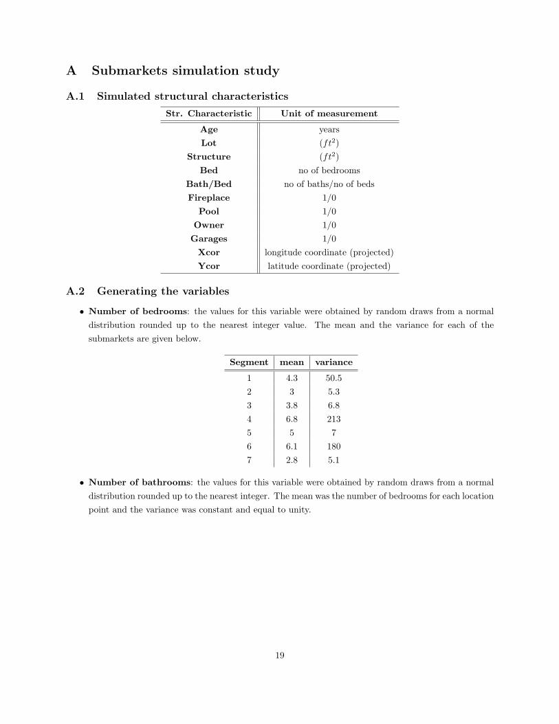
A.1 Simulated structural characteristics

Str. Characteristic Unit of measurement

Age yearsLot (ft2)

Structure (ft2)Bed no of bedrooms

Bath/Bed no of baths/no of bedsFireplace 1/0

Pool 1/0Owner 1/0

Garages 1/0Xcor longitude coordinate (projected)Ycor latitude coordinate (projected)

A.2 Generating the variables

• Number of bedrooms: the values for this variable were obtained by random draws from a normaldistribution rounded up to the nearest integer value. The mean and the variance for each of thesubmarkets are given below.

Segment mean variance

1 4.3 50.52 3 5.33 3.8 6.84 6.8 2135 5 76 6.1 1807 2.8 5.1

• Number of bathrooms: the values for this variable were obtained by random draws from a normaldistribution rounded up to the nearest integer. The mean was the number of bedrooms for each locationpoint and the variance was constant and equal to unity.

19

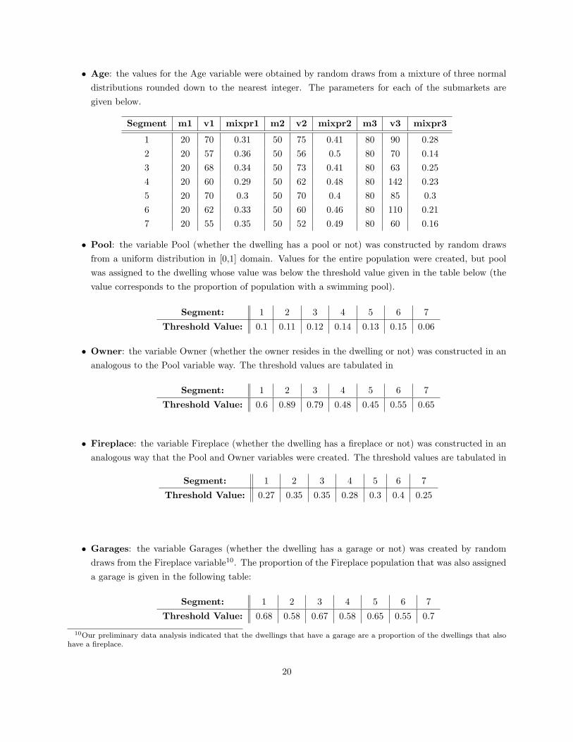
• Age: the values for the Age variable were obtained by random draws from a mixture of three normaldistributions rounded down to the nearest integer. The parameters for each of the submarkets aregiven below.

Segment m1 v1 mixpr1 m2 v2 mixpr2 m3 v3 mixpr3

1 20 70 0.31 50 75 0.41 80 90 0.282 20 57 0.36 50 56 0.5 80 70 0.143 20 68 0.34 50 73 0.41 80 63 0.254 20 60 0.29 50 62 0.48 80 142 0.235 20 70 0.3 50 70 0.4 80 85 0.36 20 62 0.33 50 60 0.46 80 110 0.217 20 55 0.35 50 52 0.49 80 60 0.16

• Pool: the variable Pool (whether the dwelling has a pool or not) was constructed by random drawsfrom a uniform distribution in [0,1] domain. Values for the entire population were created, but poolwas assigned to the dwelling whose value was below the threshold value given in the table below (thevalue corresponds to the proportion of population with a swimming pool).

Segment: 1 2 3 4 5 6 7

Threshold Value: 0.1 0.11 0.12 0.14 0.13 0.15 0.06

• Owner: the variable Owner (whether the owner resides in the dwelling or not) was constructed in ananalogous to the Pool variable way. The threshold values are tabulated in

Segment: 1 2 3 4 5 6 7

Threshold Value: 0.6 0.89 0.79 0.48 0.45 0.55 0.65

• Fireplace: the variable Fireplace (whether the dwelling has a fireplace or not) was constructed in ananalogous way that the Pool and Owner variables were created. The threshold values are tabulated in

Segment: 1 2 3 4 5 6 7

Threshold Value: 0.27 0.35 0.35 0.28 0.3 0.4 0.25

• Garages: the variable Garages (whether the dwelling has a garage or not) was created by randomdraws from the Fireplace variable10. The proportion of the Fireplace population that was also assigneda garage is given in the following table:

Segment: 1 2 3 4 5 6 7

Threshold Value: 0.68 0.58 0.67 0.58 0.65 0.55 0.7

10Our preliminary data analysis indicated that the dwellings that have a garage are a proportion of the dwellings that alsohave a fireplace.

20

• lot: the values for the variable lot (the surface of the dwelling’s lot in ft2) were obtained by randomdraws from a normal distribution whose mean and variance, for each of the submarkets, are givenbelow.

Segment Mean Variance

1 11000 90000002 6800 40000003 8500 62500004 15000 250000005 10000 84000006 14000 250000007 6000 3240000

• Structure: the variable structure (the surface of the dwelling’s structural area in ft2) is constructedby a linear combination of the number of bedrooms, the number of bathrooms, and the lot area plusa constant term. The corresponding parameters are tabulated below.

Segment Constant No of Bedrooms No of Bathrooms Lot Area

1 446.3 123.8 485.8 0.00332 57.3 211.2 371.9 0.00893 486 168.8 374.1 0.001794 207.5 97.2 637.3 0.006055 400 120 450 0.0046 200 92 610 0.00637 58 200 380 0.01

• Xcor: the variable Xcor (the longitude coordinate) was originally set to take values from 1 to 500(each integer value to correspond to one unit of longitude). In order to be conformable with real-worldcoordinate values, it was transformed to take values from (-119 (=0) to -117.5 (=500)).

• Ycor: the variable Ycor (the latitude coordinate) was originally set to take values from 1 to 500(each integer value to correspond to one unit of latitude). In order to be conformable with real-worldcoordinate values, it was transformed to take values from (33.3 (=0) to 34.5 (=300)).

• Xcor2: the square of the Xcor variable

• Ycor2: the square of the Ycor variable

21

• Sales value: the logarithm of the sales values for each dwelling constructed according to (23) in themain text. The parameter values for each submarket are provided in the following table.

Segment Constant lot structure Age Bed Bath/Bed Fireplace

1 10000 0.000004 0.000200 0.0008 -0.04 -0.015 0.152 -4300 0.000005 0.000150 -0.0023 -0.033 0.009 0.213 -3000 0.000005 0.000150 -0.0009 -0.013 0.11 0.254 17000 0.000048 0.000029 -0.0015 0.035 0.15 0.25 10250 0.000006 0.000150 -0.001 0.028 0.1 0.186 15000 0.000055 0.000035 -0.002 0.04 0.13 0.227 -4500 0.000005 0.000170 -0.0028 -0.038 0.01 0.18

Segment Garages Pool Owner Xcor Xcor2 Ycor Ycor2

1 0.32 0.54 0.175 240 1.009 245.5 -3.522 0.17 0.19 0.1 -45 -0.195 98.1 -1.43 0.1 0.23 0.065 -18.48 -0.08 115 -1.74 0.14 0.39 -0.23 360.2 1.52 253.9 -3.75 0.35 0.5 0.16 242 1.008 245.5 -3.516 0.15 0.4 -0.2 341.1 1.5 251.2 -3.67 0.16 0.16 0.08 -48.88 -0.21 100 -1.5

22

B Tables

B.1 Simulation Results: IID case

Case I: Low Variance

No of Distributions 3 No of Points 15382

Distribution index Mean Standard Deviation Mixing Probability

1 240000 4000 0.50

2 200000 4000 0.25

3 280000 4000 0.25

Case I: Estimates

1 240015.58 3993.14 0.4582

2 199962.23 4027.90 0.2676

3 280010.49 4066.32 0.2742

Table 1

Case II: Medium Variance

No of Distributions 3 No of Points 15382

Distribution index Mean Standard Deviation Mixing Probability

1 280000 10000 0.50

2 200000 10000 0.25

3 240000 10000 0.25

Case II: Estimates

1 279532.86 10524.22 0.2816

2 200215.38 10316.60 0.2706

3 239871.75 9537.06 0.4478

Table 2

Case III: High Variance

No of Distributions 3 No of Points 15382

Distribution index Mean Standard Deviation Mixing Probability

1 240000 20000 0.50

2 280000 20000 0.25

3 200000 20000 0.25

Case III: Estimates

1 236801.03 16331.80 0.3705

2 275602.01 21342.55 0.3558

3 199105.13 19204.50 0.2737

Table 3

23

B.2

Sim

ula

tion

Resu

lts:

Subm

ark

ets

case

Cou

nts

Iden

t/T

rue

12

34

56

7n

oob

s1

535

1571

1169

119

765

4302

1135

400

254

012

061

5492

4153

2984

1214

055

320

3517

1416

5025

9432

5224

1126

94

200

6610

625

0727

895

6296

410

227

308

692

3519

9821

144

624

216

2072

4133

2710

504

6734

78

102

119

229

no

obs

7065

5890

2735

228

9430

531

1523

226

5691

620

Fre

qu

enci

esId

ent/

Tru

e1

23

45

67

tota

l1

0.07

%59

.68%

26.0

0%23

.88%

64.7

4%28

.24%

0.41

%38

.64%

27.

64%

2.04

%22

.50%

3.18

%13

.60%

19.5

9%0.

45%

15.3

4%3

0.00

%34

.55%

6.27

%57

.01%

8.50

%21

.35%

0.90

%12

.30%

42.

83%

0.00

%0.

24%

0.35

%0.

00%

0.04

%94

.39%

3.04

%5

89.1

2%0.

07%

37.3

9%10

.64%

2.27

%23

.10%

3.69

%23

.08%

60.

34%

3.67

%7.

58%

1.42

%10

.90%

6.89

%0.

15%

7.35

%7

0.00

%0.

00%

0.03

%3.

52%

0.00

%0.

78%

0.00

%0.

25%

tota

l8%

6%30

%3%

33%

17%

3%10

0%

Tab

le4:

Hig

hE

rror

Var

ian

ce

24

Cou

nts

Iden

t/T

rue

12

34

56

7n

oob

s1

139

659

325

2427

402

1215

31

241

441

13

1299

3479

176

1194

819

754

1888

14

1829

344

6686

6480

2269

913

621

582

824

6260

8525

1930

2512

1275

36

6080

8492

294

127

2753

7817

824

715

8022

4728

260

4013

555

1150

98

2694

2331

1809

3416

3611

2013

881

no

obs

7065

5890

2735

228

9430

531

1523

226

5691

620

Fre

qu

enci

esId

ent/

Tru

e1

23

45

67

tota

l1

1.97

%0.

00%

0.24

%0.

31%

0.00

%0.

02%

95.0

3%2.

99%

20.

00%

0.00

%0.

04%

5.29

%0.

00%

1.58

%0.

15%

0.45

%3

0.00

%22

.05%

12.7

2%6.

08%

39.1

3%12

.97%

0.15

%20

.61%

40.

25%

4.97

%16

.33%

2.97

%21

.22%

14.9

0%0.

34%

14.8

7%5

11.7

2%0.

41%

22.8

9%2.

94%

8.25

%19

.86%

0.45

%13

.92%

686

.06%

0.00

%31

.05%

10.1

6%0.

42%

18.0

7%2.

94%

19.4

5%7

0.00

%26

.83%

8.22

%9.

74%

19.7

8%8.

90%

0.19

%12

.56%

80.

00%

45.7

4%8.

52%

62.5

1%11

.19%

23.7

1%0.

75%

15.1

5%to

tal

8%6%

30%

3%33

%17

%3%

100%

Tab

le5:

Low

Err

orV

aria

nce

25

Tru

eR

egio

ns

Max

Pro

por

tion

12

34

56

7H

igh

Err

orV

aria

nce

89%

60%

37%

57%

65%

28%

94%

Low

Err

orV

aria

nce

86%

46%

31%

63%

39%

24%

95%

Tab

le6:

Max

imu

mco

nce

ntr

atio

nof

iden

tifi

edre

gion

sp

oints

per

tru

ere

gion

Tru

eR

egio

ns

adju

sted

R2

All

obs

12

34

56

7H

igh

Err

orV

aria

nce

0.70

50.

861

0.51

50.

597

0.84

60.

965

0.94

20.

465

Low

Err

orV

aria

nce

0.71

40.

994

0.96

40.

974

0.99

30.

999

0.99

80.

956

no

obse

rvat

ion

s91

620

7065

5890

2735

228

9430

531

1523

226

56Id

enti

fied

Reg

ion

sad

just

edR

21

23

45

67

8H

igh

Err

orV

aria

nce

0.98

40.

986

0.97

60.

910

0.92

30.

999

0.71

3n

an

oob

serv

atio

ns

3540

014

055

1126

927

8921

144

6734

229

na

Low

Err

orV

aria

nce

0.94

10.

762

0.99

60.

994

0.98

30.

941

0.99

80.

977

no

obse

rvat

ion

s27

4041

118

881

1362

112

753

1782

411

509

1388

1

Tab

le7:

Reg

ion

Reg

ress

ion

sad

just

edR

2

26

B.3 Data Filtering results

Dwellings left Dwellings left

No filtering 166212 Structure 128936Value 137561 Bedrooms 123659

Age 133570 Bathrooms 123624Lot 129381 Geocoding 108488

27

B.4

Real

Data

Resu

lts:

Sum

mary

Sta

tist

ics

Su

mm

ary

Sta

tist

ics:

Un

segm

ente

dM

arke

tV

alu

esA

geB

ath

room

sB

edro

oms

Fir

epla

ceG

arag

esP

ool

Lot

size

Str

uct

ure

Siz

eO

wn

erM

in.

100

01

10

00

411

40

Q1

1860

0026

12

00

042

3011

011

Med

ian

2625

0047

23

01

060

7514

201

Mea

n34

3600

45.6

82.

438

3.30

50.

3465

0.50

920.

1096

7591

1810

0.86

33Q

339

4000

613

41

10

7680

1928

1M

ax10

5900

0019

912

412

41

41

8573

0018

7000

1

Tab

le8:

Su

mm

ary

Sta

tist

ics

Cor

rela

tion

Mat

rix:

Un

segm

ente

dm

arke

tV

alu

eag

eb

ath

bed

fire

pla

cega

rage

sp

ool

lot

stru

ctu

reow

ner

Val

ue

1.00

00.

003

0.42

20.

381

0.19

50.

085

0.24

00.

181

0.49

0-0

.116

age

0.00

31.

000

-0.1

17-0

.025

0.17

60.

281

-0.0

46-0

.009

-0.0

42-0

.116

bat

h0.

422

-0.1

171.

000

0.87

5-0

.073

-0.1

670.

089

0.11

30.

882

-0.2

60b

ed0.

381

-0.0

250.

875

1.00

0-0

.035

-0.0

860.

093

0.12

40.

836

-0.2

63fi

rep

lace

0.19

50.

176

-0.0

73-0

.035

1.00

00.

600

0.26

50.

077

-0.0

040.

099

gara

ges

0.08

50.

281

-0.1

67-0

.086

0.60

01.

000

0.18

40.

044

-0.1

040.

143

pool

0.24

0-0

.046

0.08

90.

093

0.26

50.

184

1.00

00.

130

0.13

50.

041

lot

0.18

1-0

.009

0.11

30.

124

0.07

70.

044

0.13

01.

000

0.17

2-0

.040

stru

ctu

re0.

490

-0.0

420.

882

0.83

6-0

.004

-0.1

040.

135

0.17

21.

000

-0.2

47ow

ner

-0.1

16-0

.116

-0.2

60-0

.263

0.09

90.

143

0.04

1-0

.040

-0.2

471.

000

Tab

le9:

Cor

rela

tion

Mat

rix

28

B.5

Real

Data

Resu

lts:

Identi

fied

regio

ns

Mea

nV

alu

es:

Seg

men

ted

Mar

ket

Iden

t.R

egio

nV

alu

esA

geB

ath

room

sB

edro

oms

Fir

epla

ceG

arag

esP

ool

Lot

size

Str

uct

ure

Siz

eO

wn

er1

7817

0049

.18

3.79

24.

374

0.27

040.

3377

0.11

8312

540

2871

0.60

072

2662

0045

.29

2.21

93.

110.

3488

0.52

950.

107

6737

1600

0.89

283

6339

0046

.69

3.01

63.

829

0.35

460.

452

0.11

8697

7324

360.

796

418

3200

48.7

16.

108

6.88

40.

2773

0.41

950.

134

2437

049

170.

4849

All

obs

3436

0045

.68

2.43

83.

305

0.34

650.

5092

0.10

9675

9118

100.

8633

Tab

le10

:M

ean

Val

ues

for

the

Iden

tifi

edS

ub

mar

kets

.

All

obse

rvat

ion

sC

lust

er1

Clu

ster

2C

lust

er3

Clu

ster

4C

oeffi

cien

tsE

stim

ate

Pr(>|t|

)E

stim

ate

Pr(>|t|

)E

stim

ate

Pr(>|t|

)E

stim

ate

Pr(>|t|

)E

stim

ate

Pr(>|t|

)(I

nte

rcep

t)-3

224

4.14

E-1

110

040

0.10

91-4

319

<2e

-16

-309

61.

8E-1

517

050

0.18

29lo

t3.

68E

-06

<2e

-16

3.81

E-0

62.

75E

-11

4.99

E-0

6<

2e-1

64.

68E

-06

<2e

-16

4.84

E-0

6<

2e-1

6st

ruct

ure

9.31

E-0

5<

2e-1

61.

73E

-04

<2e

-16

1.49

E-0

4<

2e-1

61.

48E

-04

<2e

-16

2.89

E-0

55.

97E

-06

age

-0.0

017

<2e

-16

0.00

080.

3804

-0.0

024

<2e

-16

-0.0

009

<2e

-16

-0.0

015

0.48

75b

ed0.

0093

4.68

E-1

6-0

.039

43.

02E

-08

-0.0

033

0.00

08-0

.013

1<

2e-1

60.

0343

1.78

E-0

9b

athb

ed0.

1305

<2e

-16

-0.0

152

6.51

E-0

10.

0890

<2e

-16

0.11

22<

2e-1

60.

1508

6.59

E-0

9ga

rage

s0.

1150

<2e

-16

0.14

810.

0298

720.

2127

<2e

-16

0.25

32<

2e-1

60.

2044

0.12

93p

ool

0.24

18<

2e-1

60.

3191

3.17

E-0

70.

1716

<2e

-16

0.09

88<

2e-1

6-0

.052

90.

6534

fire

pla

ce0.

2685

<2e

-16

0.54

222E

-13

0.18

74<

2e-1

60.

2263

<2e

-16

0.38

910.

0095

own

er0.

0841

<2e

-16

0.17

770.

0001

0.09

80<

2e-1

60.

0643

<2e

-16

-0.2

274

0.02

20X

cor

-24.

7200

0.00

2124

0.40

000.

0209

-44.

9000

<2e

-16

-18.

9200

0.00

3236

1.10

000.

0878

Xco

r210

2.50

00<

2e-1

61.

0230

0.02

01-0

.188

0<

2e-1

6-0

.077

20.

0044

1.52

800.

0876

Yco

r-0

.102

00.

0027

241.

6000

1.55

E-1

297

.130

0<

2e-1

611

4.90

00<

2e-1

625

2.20

000.

0001

Yco

r2-1

.509

0<

2e-1

6-3

.563

01.

17E

-12

-1.4

290

<2e

-16

-1.6

930

<2e

-16

-3.7

070

0.00

01R

20.

3005

no

obs

0.26

65n

oob

s0.

5811

no

obs

0.81

27n

oob

s0.

3863

no

obs

adju

sted

R2

0.30

0410

8488

0.26

3836

360.

581

8592

40.

8126

1796

50.

3779

963

Tab

le11

:R

egre

ssio

nE

stim

ates

29

C Figures

C.1 IID case

Figure 1: Low Variance

Figure 2: Medium Variance

30

Figure 3: High Variance

31

C.2 Submarkets case

Figure 4: Complex Submarkets

Figure 5: High Error Variance

32

Figure 6: Low Error Variance

33

C.3 Real Data: Los Angeles

Figure 7: Los Angeles County Map

34

Figure 8: Los Angeles 2002 Submarkets

35

Research Papers 2010

2010-39: Rasmus Tangsgaard Varneskov: The Role of Dynamic Specification in

Forecasting Volatility in the Presence of Jumps and Noisy High-Frequency Data

2010-40: Antonis Papapantoleon and David Skovmand: Picard Approximation of Stochastic Differential Equations and Application to Libor Models

2010-41: Ole E. Barndorff–Nielsen, Fred Espen Benth and Almut E. D. Veraart: Modelling electricity forward markets by ambit fields

2010-42: Robinson Kruse and Philipp Sibbertsen: Long memory and changing persistence

2010-43: Dennis Kristensen: Semi-Nonparametric Estimation and Misspecification Testing of Diffusion Models

2010-44: Jeroen V.K. Rombouts and Lars Stentoft: Option Pricing with Asymmetric Heteroskedastic Normal Mixture Models

2010-45: Rasmus Tangsgaard Varneskov and Valeri Voev: The Role of Realized Ex-post Covariance Measures and Dynamic Model Choice on the Quality of Covariance Forecasts

2010-46: Christian Bach and Stig Vinther Møller: Habit-based Asset Pricing with Limited Participation Consumption

2010-47: Christian M. Dahl, Hans Christian Kongsted and Anders Sørensen: ICT and Productivity Growth in the 1990’s: Panel Data Evidence on Europe

2010-48: Christian M. Dahl and Emma M. Iglesias: Asymptotic normality of the QMLE in the level-effect ARCH model

2010-49: Christian D. Dick, Maik Schmeling and Andreas Schrimpf: Macro Expectations, Aggregate Uncertainty, and Expected Term Premia

2010-50: Bent Jesper Christensen and Petra Posedel: The Risk-Return Tradeoff and Leverage Effect in a Stochastic Volatility-in-Mean Model

2010-51: Christos Ntantamis: A Duration Hidden Markov Model for the Identification of Regimes in Stock Market Returns

2010-52: Christos Ntantamis: Detecting Structural Breaks using Hidden Markov Models

2010-53: Christos Ntantamis: Detecting Housing Submarkets using Unsupervised Learning of Finite Mixture Models